A Model for Quantum Stochastic Absorption in Absorbing Disordered Media

Abstract

Wave propagation in coherently absorbing disordered media is generally modeled by adding a complex part to the real part of the potential. In such a case, it is already understood that the complex potential plays a duel role; it acts as an absorber as well as a reflector due to the mismatch of the phase of the real and complex parts of the potential. Although this model gives expected results for weakly absorbing disordered media, it gives unphysical results for the strong absorption regime where it causes the system to behave like a perfect reflector. To overcome this issue, we develop a model here using stochastic absorption for the modeling of absorption by $``$fake$"$, or $``$side$"$, channels obviating the need for a complex potential. This model of stochastic absorption eliminates the reflection that is coupled with the absorption in the complex potential model and absorption is proportional to the magnitude of the absorbing parameter. Solving the statistics of the reflection coefficient and its phase for both the models, we argue that stochastic absorption is a potentially better way of modeling absorbing disordered media.

]

I introduction

Quantum and classical wave propagation and localization in disordered media is a well studied problem [2, 3, 4]. Recently in the literature, more attention has been paid to studying the effect of localization on coherent absorption/amplification in coherently absorbing/amplifying disordered media, both theoretically [5, 6, 7, 8, 9, 10, 11, 12] and experimentally [13, 14, 15, 16, 17, 18, 19]. Light is Bosonic, so it can be amplified or absorbed. On the other hand, electrons are Fermions, which can not be amplified; however, they can be absorbed in the sense of phase de-coherence. Coherent absorption/amplification in a coherently absorbing/amplifying medium is a non-conserving scattering process where temporal phase coherence of a wave is preserved despite absorption/amplification. Coherent back scattering (CBS) in a disordered medium, the main cause of weak and strong localization, is not affected by the additional presence of a coherently absorbing/amplifying medium due to the persistence of phase coherence of the interfering waves. It was shown [5] that the localization can enhance the coherent light amplification in a coherently amplifying (i.e. lasing) disordered medium, resulting in a self-sustaining mirror-less lasing action where coherent feed back for lasing action is supported by disorder induced localization. In that same frame work, we also studied the effect of localization on the coherently absorbing disordered media and showed the similarities of the two processes for effective localization and effective active lengths. This problem studied further in detail by different approaches [7, 8, 9, 10, 11, 12]. The general approach to model coherent amplification and absorption is to add a constant complex part to the real part of the potential. Depending on the sign of the complex potential, the model shows amplification or absorption. Modeling absorption/amplification by a complex potential, however, always gives a reflection part due to the mismatch between the real and the imaginary potentials. Studying a delta scatterer, which has both real and complex parts, it was shown [20] that absorption is not a monotonic function of the strength of the complex potential. Although complex potential model works well for the case of weakly absorbing/amplifying disordered media, it gives unphysical results in the strong absorption/amplification regime because the system behaves like a perfect reflector. To address this issue, it was derived and demonstrated [6] that absorption without reflection can be modeled by using a stochastic absorption model. Recent detailed numerical studies have been performed by transfer matrix methods [21, 22] to study our approach, and the numerical results support our model. Here, we first study the coherently absorbing disordered media modeled by a adding complex potential. Then, we present a detailed derivation and analysis of the Langevin equation in case of stochastic absorption for the modeling of absorption by $``$fake$"$, or $``$side$"$, channels obviating the need for a complex potential. We show that stochastic absorption model gives potentially better physical results than the model by a complex potential for transport in 1D absorbing disordered media in the regime of strong absorption. However, these two models give the same result for weak disorder and the weakly absorbing regime.

II Coherent Absorption Modeled by Complex Potentil

There has been recent interest in the role of absorption in localization, and on the different length scales in the problem in the presence of absorption. For the bosonic case, like light etc., a coherent state (e.g. a laser beam) is an eigenstate of the annihilation operator. Removal of a photon(absorption) does not destroy the phase coherence. Fermions cannot be annihilated in the context we are considering here. For the Fermionic case, the physical picturization of the absorption will be some kind of inelastic process (like scattering by phonons), where electrons lose their partial temporal phase memory. This type of absorption is called stochastic absorption.

Recent theoretical studies [23, 24, 25] have shown that the absorption in the case of light waves does not give any cut-off length scale for the localization problem. If a system is in the localized state, absorption will not kill the localization to make the system again diffusive. A sharp mobility edge exists even in the presence of significant absorption in 3D.

Adding a constant imaginary part with the proper sign to the real potential of the Maxwell/Schrödinger wave equation can model the linear coherent absorption/amplification. Both the Maxwell and the Schrödinger equations can be transformed to the form of the Helmholtz equation. A general form of a Helmholtz equation can be written as:

$$\frac{\partial^{2}u}{\partial x^{2}}+k^{2}[1+(\eta(x)+i\eta_{a})]u\,=0\quad,$$ (1)

For the electronic case, consider $V(x)+iV_{a}$ as the potential, $k$ as the wave vector, and $\hbar/2m=1$. For the optical case, consider $\epsilon_{0}+i\epsilon_{a}$ as the constant dielectric background and $\epsilon(x)$ as the randomly spatially fluctuating part of the dielectric constant, $k\equiv 2\pi/\lambda$, where $\lambda=$ wavelength in the average medium $(\epsilon_{0})$. Then, we can define $\eta(x)$=$-V(x)/k^{2}$, $\eta_{a}$=$-V_{a}/k^{2}$ for the Schrödinger equation, and $\eta(x)$= $+{\epsilon(x)\over\epsilon_{0}}$, $\eta_{a}$= $+{\epsilon_{a}\over\epsilon_{0}}$ and $k^{2}={\omega^{2}\over c^{2}}\epsilon_{0}$ for the Maxwell equation.

The model we are considering here is for a one-channel scalar wave where the polarization aspects have been ignored. This holds well for a single-mode polarization maintaining optical fiber. For electronic case, we consider only a single channel.

As pointed out in Ref [20], modeling absorption by a complex potential will always give a concomitant reflection. Absorption is not possible without reflection and there is a competition between the absorption and the reflection. For very high absorption, the system may try to act as a perfect reflector. We extend and explore this idea for coherently absorbing 1-D disordered media. The Langevin equation for the complex amplitude reflection coefficient $R(L)$ can be derived by the invariant imbedding method [26] from the Helmholtz equation Eq.(1),

$$\frac{dR(L)}{dL}\,=\,\,2ikR(L)\,+\,i\frac{k}{2}(1+\eta(L)+i\eta_{a})(1+R(L))^{2}\quad,$$ (2)

with the initial condition R(L)=0 for L=0.

Now, taking $R(L)=\sqrt{r}e^{i\theta}$, the Langevin equation Eq.(2) reduces to two coupled differential equations in $r$ and $\theta$. For a Gaussian white noise potential, using a stochastic Liouville equation for the evolution of probability density and then integrating out the stochastic part by Novikov’s theorem, we get the Fokker-Planck equation:

$$\frac{\partial P(r,\theta)}{\partial l} = \left[\sin\theta\frac{\partial}{\partial r}(r^{1/2}(1-r))+\frac{\partial}{\partial\theta}\right.$$ (8)

$$\left.+{1\over 2}(r^{1/2}+r^{-1/2})\frac{\partial}{\partial\theta}cos(\theta)\right]^{2}P(r,\theta)$$

$$-2k\xi\frac{\partial}{\partial\theta}\left[P(r,\theta)\right]$$

$$+D\frac{\partial}{\partial r}\left[rP(r,\theta)\right]$$

$$+{D\over 2}\cos\theta\frac{\partial}{\partial r}\left[r^{1/2}(1+r)P(r,\theta)\right]$$

$$+{D\over 4}(r^{1/2}-r^{-1/2})\frac{\partial}{\partial\theta}\left[\sin\theta P(r,\theta)\right]\quad,$$

where we have introduced the dimensionless length $l=\frac{L}{\xi}$ and $D=\frac{4\eta_{a}}{qk}$ = $\xi/\xi_{a}$, and $\xi\equiv({1\over 2}qk^{2})^{-1}$ is the localization length and $\xi_{a}={1\over 2k\eta_{a}}$ is the absorbing length scale in the problem, and $q$ is the strength of the delta correlation of the random potential.

The Fokker-Planck equation Eq.(8) can be solved analytically for the asymptotic limit of large lengths in the random phase approximation (i.e., for the weak disorder case). Then, the statistics $P^{D}(r,l)$ have a steady state distribution for $l\rightarrow\infty$. It can be obtained by setting $\partial P(r,l)/\partial l=0$ and solving the resulting equation analytically. We get [5] the following steady state distribution:

$$\lim_{l\rightarrow\infty\atop}P^{D}(r,l) = \left\{\begin{array}[]{cl}\frac{|D|exp(|D|)exp(-{|D|\over 1-r})}{(1-r)^{2}}&\quad\mbox{for}\;r\leq 1\\ 0&\quad\mbox{for}\;r>1,\end{array}\right.$$ (11)

For $D=0$ and $l\rightarrow\infty$, equation (8) reduces to a half delta function peaked around $r=1$. The Fokker-Planck equation, Eq.(8), is difficult to solve analytically beyond the random phase approximation. We solve the full Fokker-Planck equation (8) numerically to calculate the statistics of the reflection coefficient and its phase in a regime of strong disorder with strong absorption.

To see the actual evaluation of the probability as a function of reflection coefficent for a fixed disorder strength and length, we evolved the full Fokker-Planck equation without approximation. The Fokker-Planck equation is solved as an initial value problem, i.e. $P(r,l=0)=\delta(r=0)$.

In Fig.1 we plot the results of our numerical simulations. The $P(r)$ distributions show (top plot) that for the strongly absorbing disordered media, the probability initially peaks near $r=0$ and the peak slowly moves towards $r=1$ for larger sample lengths, indicating stronger reflection for stronger absorption. In Fig.1, the bottom plot shows that the steady state phase distribution is a delta function peaking symmetrically about $\theta=\pi$.

These plots, show the system behaving as a perfect reflector for higher lengths, with strong disorder and strong

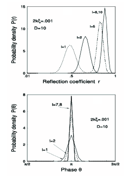
FIG. 1.: Probability distribution $P(r)$ and $P(\theta)$ separately against the sample length $l$. Parameters are fixed strong disorder strength $2k_{F}\xi=.001$ and fixed strong absorbing parameter $|D|=10$.

absorbing parameter $|D|$. Therefore, this coherent absorbing model is restricted for the weakly absorbing parameter regime.

III Stochastic Absorption

In the previous section, we have shown and discussed that the absorption is not possible without reflection in a calculation where absorption is modeled by adding a constant imaginary potential to the real potential. In the Langevin equation for $R(L)$, derived from these types of models, the wave always gets a reflected part along with the absorption. There is, however, another way of deriving a Langevin equation for the reflection amplitude $R(L)$ such that the absorption does not have a concomitant reflected part. This approach is motivated by the work of references [27, 28] where some purely absorptive $``$fake$"$ (side) channels are added to the purely elastic scattering channels of interest. A particle that once enters to the absorbing channel, never comes back and it is physically lost. We derive the Langevin equation for $R(L)$ following the approach in Ref.[27]. This Langevin equation has some formal differences from Eq.(2). However,

FIG. 2.: Modeling $``$absorption$"$ by fake channels: Channels 1 and 2 are coupled through the current leads to two ”fake” channels 3 and 4 which connect to a thermal reservoir.

it does not differ for the weak disorder case.

Now we proceed to derive Langevin equation for $R(L)$ using the $``$fake$"$ channel approach. The main idea is to simulate absorption by enlarging the S-matrix to include some $``$fake$"$, or $``$side$"$ channels that remove some probability flux out of reckoning. Let us assume that the scatterer has a general scattering channel and an absorbing channel ending with a phase randomizer which acts as a blackbody. The scattering matrix can be taken as discussed in reference [27]. Consider scattering channels 1 and 2 connected through current leads to two quantum $``$fake$"$ channels 3 and 4 that carry electrons to the reservoir, ( with chemical potential $\mu$) as shown in Fig.2 (for only one scatterer). This is a phenomenological way of modeling absorption [27, 28]. Electrons entering into the channels 3 and 4 are absorbed regardless of their phase and energy. The absorption is proportional to the strength of the $``$coupling parameter$"$ $\epsilon$. A symmetric scattering matrix $S$ for such a system can be written as :

$$\left(\begin{array}[]{cccc}\alpha R&\alpha T&0&\beta\\ \alpha T&\alpha R&\beta&0\\ 0&\beta&-\alpha R^{*}&-\alpha T^{*}\\ \beta&0&-\alpha T^{*}&-\alpha R^{*}\end{array}\right)\quad,$$ (12)

where $R$ and $T$ are the reflection and the transmission amplitudes for the single scatterer , $\alpha=\sqrt{1-\epsilon}$ is the absorption coefficient, and $\beta=\sqrt{\epsilon}$.

Now, the full scattering matrix is unitary for all positive real $\epsilon<1$. But the sub-matrix directly connecting only the channels 1 and 2 is not unitary. We will now explore this fact in our derivation. We observe from the above sub-matrix that for every scattering involving channels 1 and 2 only the reflection and the transmission amplitudes get multiplied by $\alpha$ (the absorption parameter). Now keeping this fact in mind, we will derive the Langevin equation for the reflection amplitude $R(L)$ for $N$ scatterers (of length L) each characterized by a random S-matrix of this type, with the same $\alpha$ value.

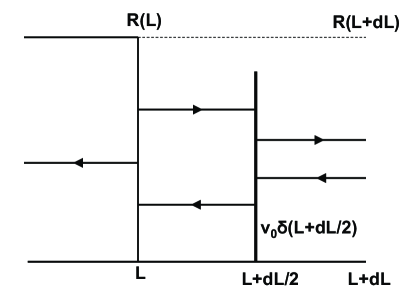
FIG. 3.: A schematic picture of a scatterer of length $L$ having reflection amplitude $R(L)$ while an added length $dL$ makes the length of the scatterer $L+dL$. The effective potential of the length $dL$ is shown by an effective summary delta-function potential.

Consider $N$ random scatterers for a 1D sample of length $L$ with $(\equiv Na,a\equiv unitspacing)$ the reflection amplitude $R(L)$, and $N+1$ scatterers of the sample length $L+\triangle L$, with the reflection amplitude $R(L+\triangle L)$. That is, let us start with the $N$ scatterers, and add one more scatterer to the right to make up the N+1 scatterers. Now, we want to see the relation between $R(L)$ and $R(L+\triangle L)$. That is, let there be a delta-function potential scatterer between $L$ and $L+\triangle L$, positioned at the point $L+\triangle L/2$, that can be considered as the effective scatterer due to the extra added scatterers for length $\triangle L$. For $k\triangle L\ll 1$, we can treat the extra added scatterer as an effective delta potential $v_{0}(L)\delta(x-L-\triangle L/2)$ with $v_{0}(L)=V(L)\triangle L$.(We consider the continuum limit, $a\rightarrow 0$, $N\rightarrow\infty$, and $Na=L$ fixed ).

Now, for a plane-wave scattering problem for a delta function potential of strength $v_{0}$, which is at $x=0$ and has complex reflection and transmission amplitudes $r_{0}$ and $t_{0}$ respectively, we have from the continuity condition for the wave function and discontinuity condition for the derivative of the wave function (which one gets by integrating the Schrödinger equation across the delta function):

$$r_{0}=\frac{v_{0}}{i2k-v_{0}}\quad\mbox{and}\quad t_{0}=r_{0}+1.$$ (13)

Considering $v_{0}=v(L)\triangle L$ the smallness parameter, one gets expressions up to first order in $\triangle L$ for $r_{0}$ and $t_{0}$:

$$r_{0}=\frac{v_{0}}{2ik}\quad\mbox{and}\quad t_{0}=1+\frac{v_{0}}{2ik},$$ (14)

where we have taken $\hbar^{2}/2m=1$.

Now to introduce absorption we will write:

$$r \rightarrow r\alpha=r_{0}(1-\epsilon)^{1/2},$$ (15)

$$t \rightarrow t\alpha=t_{0}(1-\epsilon)^{1/2}.$$ (16)

This means that for every scattering the reflection and transmission amplitudes get modulated by a factor of ${\alpha}$.

Now consider a plane wave incident on the right side of the sample of length $L+\triangle L$. Summing all the processes of direct and multiple reflections and transmissions, on the right side of the sample of length $L$, with the effective delta potential at $L+\triangle L/2$, we get,

$$R(L+\triangle L) = re^{ik\triangle L}$$ (17)

$$+ e^{ik\triangle L/2}te^{ik\triangle L/2}R(L)e^{ik\triangle L/2}te^{ik\triangle L/2}$$ (18)

$$+ .......\,.$$ (19)

Summing the above geometric series, substituting the values of $r$ and $t$, and taking the continuum limit for L , one gets from Eq.(19), the Langevin equation:

$$\frac{dR(L)}{dL}\,=\,-\alpha R(L)+2ikR(L)\,+\,i\frac{k}{2}(\eta(L))(1+R(L))^{2}\,,$$ (20)

with the initial condition $R(L)=0$ for $L=0$, and $\alpha$ is the absorbing parameter. This is not quite the same as the Eq.(2) obtained by introducing an imaginary potential. It turns out, however, that this Langevin equation gives the same results in the regime of weak disorder but differs qualitatively in the regime of strongly absorbing disordered media.

Similarly, following the same steps as we discussed previously, from the Langevin Eq.(19) we derive the Fokker-Planck equation:

$$\frac{\partial P(r,\theta)}{\partial l} = \left[\sin\theta\frac{d}{dr}(r^{1/2}(1-r))+\frac{\partial}{\partial\theta}\right.$$ (21)

$$+ \left.{1\over 2}(r^{1/2}+r^{1/2})\frac{\partial}{\partial\theta}(cos(\theta))\right]^{2}P(r,\theta)$$ (22)

$$- 2k\xi\frac{\partial P(r,\theta)}{\partial\theta}+D\frac{\partial(Pr)}{\partial r}\quad,$$ (23)

where parameters $l$ and $2k\xi$ are same as defined in Eq.(8), and $D={4\alpha\over qk}$.

In the weak disorder limit, when the phase part is integrated out by the RPA, Eq. (23) and Eq.(8) give the same Fokker-Planck equation in $r$. Hence, the steady state $P(r)$ solution for the both are same, i.e. Eq.(11). We will consider here only the strong disorder case for the numerical calculations of the Fokker-Planck equation (23), which goes beyond the RPA to compare it with the solution of Eq.(8).

Fig.4(a) is the plot of $P(r)$ for the strong disorder ($2k_{F}\xi=.001$) and strongly absorbing ($D=10$) limit, with different lengths of the sample. $P(r)$ distributions are peaked around $r=0$. The wave is absorbed in the medium before it gets reflected as we have modeled absorption without reflections and we are considering the case of strong absorption, and hence the probability of absorption is more than that of reflection.

FIG. 4.: Probability distributions (a) $P(r)$ and (b) $P(\theta)$ against the sample length $l$ with fixed strong disorder strength $2k_{F}\xi=.001$ and fixed strong stochastic absorption parameter $D=10$.

Fig.4(b) shows the phase distribution $P(\theta)$, which is a double peaked symmetric distribution and differs from the model of absorption by complex potential, which is a delta function distribution at $\theta=\pi$ as shown in Fig.1 (bottom).

IV Discussion and Conclusion

In conclusion, we have shown a comparison between the modeling of absorption in disordered medium (i) by a complex potential and (ii) by fake channel $S$ matrix approach. We derived a new Langevin equation using the latter method. We calculated the statistics of the reflection coefficient $(r)$ and its associated phase $(\theta)$ for a wave reflected from absorbing disordered media, for different disorder strengths and lengths of the sample, for the both models. For the case of weak disorder with weak absorption, i.e. within the RPA, the FP equation for the case of stochastic absorption is the same as that of the absorption modeled by a complex potential. For the regime of strong disorder with strong absorption, the stochastic absorption model behaves as a perfect absorber opposite to the coherent absorbtion case, which behaves as a perfect reflector. Therefore, the Langenvin equation derived from stochastic absorption method gives a potentially better physical model for coherent absorption. Our model proposed here has already been verified and supported by extensive numerical simulation using a transfer matrix method [21, 22].

I gratefully acknowledge N. Kumar for many stimulating discussions.

REFERENCES

- [1] e-mail pradhan@ece.northwestern.edu
- [2] P. W . Anderson, Phys. Rev. 109, 1492 (1958).
- [3] P. A. Lee and T. V. Ramakrishnan Rev. Mod. Phys. 57, 287 (1985).
- [4] For review of localization and multiple scattering see Scattering and localization of classical waves in random media, Ed. Ping Sheng (World Scientific, Singapore, 1990).
- [5] P. Pradhan and N. Kumar, Phys. Rev. B 50, 5616 (1994).
- [6] Prabhakar Pradhan, cond-mat/9807312, 1998.
- [7] Z. Q. Zhang, Phys. Rev. B 52, 7960(1995).
- [8] A. K. Gupta and A. M. Jayannavar, Phys. Rev. B 52, 4156(1995).
- [9] C. W. J. Beenakker, J. C. J. Paasschens, and P. W. Brouwer, Phys. Rev. Lett. 76, 1368 (1996).
- [10] S. K. Joshi and A. M. Jayannavar, Phys. Rev. B 56, 12038(1997).
- [11] J. Heinrichs, Phys. Rev. B 56, 8674(1997).
- [12] X. Jiang and C. M. Soukoulis, Phys. Rev. Lett. 85, 70 (2000).
- [13] M. N. Lawandy, R. M. Balachandran, A. S. L. Gomes and E. Sauvain, Nature, 368, 436 (1994).
- [14] A. Z. Ganack and J. M. Drake, Nature 368, 400 (1994).
- [15] R. M. Balachandran and M. N. Lawandy Opt. Lett. 20, 1271 (1995).
- [16] D. S. Wiersma, M. P. van Albada and A. Lagendijk, Phys. Rev. Lett. 75, 1739 (1995).
- [17] D. S. Wiersma, Ph. D. Thesis, 1995, FOM-Institute for Atomic and Molecular Physics, Amsterdam .
- [18] B. R. Prasad, H. Ramachandran, A. K. Sood, C. K. Subramanian, and N. Kumar, App. Opt. 36, 7718(1997).
- [19] H. Cao et al., Phys. Rev. Lett. 82, 2278 (1999).
- [20] A. Rubio and N. Kumar, Phys. Rev. B 47, 2420 (1993).
- [21] S.K. Joshi, D. Sahoo, and A.M. Jayannavar, Phys. Rev. B 62, 880 (2000).
- [22] S.K. Joshi and A.M. Jayannavar, cond-mat/0004132, 2000.
- [23] R. L. Weaver, Phys. Rev. B 47, 1077 (1993)
- [24] M. Yosefin, Europhys. Lett. 25, 675 (1994).
- [25] A. M. Jayannavar, Phys. Rev. B 49, 14718 (1994)
- [26] R. Rammal and B. Docout, J. Phys.(Paris) 48, 509 (1987).
- [27] M. Buttiker, Phys. Rev. B 33, 3020 (1986).
- [28] R. Hey, K. Maschke and M. Schreiber, Phys. Rev. B 52 8184 (1995).