Quantum Spin Pump in $S=1/2$ antiferromagnetic chains
-Holonomy of phase operators in sine-Gordon theory-

Abstract

In this paper, we propose the quantum spin pumping in quantum spin systems where an applied electric field ($E$) and magnetic field ($H$) cause a finite spin gap to its critical ground state. When these systems are subject to alternating electromangetic fields; $(E,H)=(\sin\frac{2\pi t}{T},\cos\frac{2\pi t}{T})$ and travel along the loop $\Gamma_{\rm{loop}}$ which encloses their critical ground state in this $E$-$H$ phase diagram, the locking potential in the sine-Gordon model slides and changes its minimum. As a result, the phase operator acquires $2\pi$ holonomy during one cycle along $\Gamma_{\rm{loop}}$, which means that the quantized spin current has been transported through the bulk systems during this adiabatic process. The relevance to real systems such as Cu-benzoate and ${\rm{Yb}}_{4}{\rm{As}}_{3}$ is also discussed.

1 Introduction

Transport phenomena in magnets such as the colossal magnetoresistance[1] and anomalous Hall effect[2, 3, 4, 5, 6, 7, 8] are long-standing subjects in solid state physics. Recently, exotic characters of the anomalous Hall effect are closed up in ferromagnets[9, 10, 11, 12], antiferromagnets[13] and spin glass[14, 15] with non-coplanar spin configurations and collinear ferromagnets with strong spin-orbit couplings[16, 17, 18, 19, 20]. Their common origin is gradually recognized as the topological character of magnetic Bloch wavefunctions in its ordered phase, sharing the same physics with the two dimensional ($2$D) quantum Hall effect. Thereby the spontaneous Hall conductivity is related to the fictitious magnetic field defined in the crystal momentum space and its quantized value is directly related to the first Chern number associated with the fiber bundle whose base space is spanned by crystal momenta.

Meanwhile, in early 80’s, Thouless and Niu proposed the quantized adiabatic particle transport (QAPT) in gapped fermi systems, where an adiabatic sliding motion of the periodic electrostatic potential in one dimensional ($1$D) system pumps up an integer number of electrons per cycle.[21, 22] In fact, this quantized particle transport is another physical manifestation of the topological character associated with the Bloch wavefunctions. Specifically this particle (polarization) current is related to the fictitious magnetic field defined in the generalized crystal momentum space which is in turn spanned by the crystal momentum and deformed parameters. Because of this analogy to the 2D quantum Hall currents, this $1$D quantized particle current is known to be topologically protected against other perturbations such as disorders and electron-electron correlations[22]. Due to this peculiar topological protection, the QAPT became recently highlighted in the realm of the spintronics, where electron pumpings have been experimentally realized in meso and/or nano-scale systems.[23, 24, 25, 26] However the quantized value observed in these experiments should be attributed to the Coulomb blockade [23, 25, 26] and is different form the aforementioned Thouless quantization, which is assured only in the thermodynamic limit.[23]

In this paper, based on the original idea of the QAPT, we propose the quantized spin transport (quantum spin pump) in the macro-scale magnets. There we discuss systematically the topological stability of its quantization. Specifically, we clarify in this paper the relation between its quantization and holonomy of the phase operator of sine-Gordon theory in $1$D quantum field theory. By using this relation, its topological stability can be quantitatively judged by seeing whether the expectation value of this phase operator acquires $2\pi$ holonomy during the cyclic process or not.

As for the experimental relevant systems to our theory of quantized spin transports, we have the $S=\frac{1}{2}$ quantum spin chain such as Cu-benzoate and ${\rm{Yb}}_{4}{\rm{As}}_{3}$ (charge ordered phase), where its unit cell contains two crystallographically inequivalent sites. Accurately speaking, both the translational symmetry by one site $(T:\mbox{\boldmath{$S$}}_{j}\rightarrow\mbox{\boldmath{$S$}}_{j+1})$ and the bond-centered inversion symmetry which exchanges the nearest neighboring sites $(I_{\rm{bond}}:\mbox{\boldmath{$S$}}_{i-j}\leftrightarrow\mbox{\boldmath{$S$}}_{i+j+1}$ are crystallographically broken. As a result of this peculiar crystal symmetry, the $g$-tensors of its two sublattices are in general different in these systems;

$$H=J\sum_{i=1}^{N}\mbox{\boldmath{$S$}}_{i}\cdot\mbox{\boldmath{$S$}}_{i+1}+$$

$$\hskip 22.76228pt\sum_{i}\mbox{\boldmath{$H$}}\cdot\bigl{[}[g_{\rm{u}}]+(-1)^{i}[g_{\rm{a}}]\bigr{]}\cdot\mbox{\boldmath{$S$}}_{i},\hskip 5.69046pt(J>0)$$ (1)

where $[g_{\rm{u}}]$ and $[g_{\rm{a}}]$ represent the uniform and staggered component of the $g$-tensors respectively.[27] Late 90’s, these quantum spin systems, whose ground states are nearly critical because of their strong one dimensionalities, are experimentally revealed to show the spin gap behaviors under the external magnetic field. Furthermore, following theoretical works showed that the field-induced gap behaviors $(\Delta\sim H^{2/3})$ are originated from this staggered component of the $g$-tensor, where the effective staggered magnetic field in the eq. (1) endows its critical ground state with a finite spin gap.[29, 30]

On the other hand, the exchange interaction $J$ in these $S=1/2$ quantum spin chains, $J\sum_{i}\mbox{\boldmath{$S$}}_{i}\cdot\mbox{\boldmath{$S$}}_{i+1}$, does not have an alternating component, since these systems are invariant under the site-centered inversion symmetry which exchanges the nearest neighbor bonds ($I_{\rm{site}}:\mbox{\boldmath{$S$}}_{i-j}\leftrightarrow\mbox{\boldmath{$S$}}_{i+j}$). However, when we break this symmetry by applying an electric field $E$ along an appropriate direction[31], the exchange interaction in general does acquire a staggered component;

$$H=\sum_{i=1}^{N}\bigl{[}J-(-1)^{i}\Delta\bigr{]}\mbox{\boldmath{$S$}}_{i}\cdot\mbox{\boldmath{$S$}}_{i+1}.$$ (2)

Futhermore a site-centered inversion operation with the sign of $E$ reversed requires that $\Delta$ must be an odd function of $E$. This dimerizing field $\Delta$ is also expected to induce a finite mass to its critical ground state, causing the spin-Peierls state.

Based on these observations, we propose a method of generating the quantized spin current in this type of spin systems ($T,I_{\rm{bond}}$ : broken, $I_{\rm{site}}$ : unbroken) by using electromagnetic fields. Specifically, we study a following $S=1/2$ Heisenberg model with time-dependent staggered field and bond alternation:

$$\hat{H}(t) = \sum_{i=1}^{N}\bigl{[}J-(-1)^{i}\Delta(t)\bigr{]}\mbox{\boldmath{$S$}}_{i}\cdot\mbox{\boldmath{$S$}}_{i+1}$$ (3)

$$\ +\ h_{\rm{st}}(t)\sum_{i=1}^{N}(-1)^{i}S^{z}_{i}.$$

where staggered Zeeman field $h_{\rm st}(t)$ and bond alternations $\Delta(t)$ are supposed to be controlled by the applied electromagnetic fields. In $\S$ 2, we will argue by using bosonization technique that the quantized number of $z$-component of spins are transported from one end of the system to the other during one cycle along the loop which encloses the critical ground state at $(\Delta,h_{\rm st})=(0,0)$ in the $\Delta$-$h_{\rm st}$ plane.

In order to uphold this bosonization argument, we also demonstrate the numerical calculations in $\S$ 3, where we evolve the ground state wavefunction according as the above time-dependent Hamiltonian. Thereby we attibute the quantized spin transport to the Landau-Zener tunnelings [40] which indeed happen between several energy levels during this cycle process.

In addition to eq.(3), we also have a uniform component of Zeeman fields in real systems,

$$H^{\prime}(t)=\sum_{j=1}^{N}\mbox{\boldmath{$H$}}(t)\cdot\mbox{\boldmath{$S$}}_{j},$$

whose magnitude is usually larger than that of the staggered component $h_{\rm st}(t)$. This uniform field, especially its $x$ or $y$ component, seems to easily flip the spins accumulated at both boundaries and might spoil the physical consequence of the spin transport. Then we also discuss in $\S$ 3 the effect of this uniform field and the remedy against it, where it turns out that the sweeping velocity should be appropriately chosen so as to avoid the relaxation process via this uniform Zeeman field.

2 Bosonization

For clarity, let us first illustrate the physics of our quantum spin pumping in a simple limiting case;

$$H_{\rm{XY}} = -\frac{J}{2}\sum_{i=1}^{N}(\hat{S}^{+}_{i}\hat{S}^{-}_{i+1}+{\rm{c.c.}}),$$ (4)

$$H_{\rm{dim}} = \frac{\Delta}{2}\sum_{i=1}^{N}(-1)^{i}\left(\hat{S}^{+}_{i}\hat{S}^{-}_{i+1}+\hat{S}^{-}_{i}\hat{S}^{+}_{i+1}\right),$$ (5)

$$H_{\rm{st}} = h_{\rm{st}}\sum_{i}(-1)^{i}\hat{S}^{z}_{i},$$ (6)

where we take the direction of the staggered Zeeman field as the $z$-direction.[32] In this simplification, we neglected the exchange coupling between the $z$-component of spins. In this limit, we can get a quadratic form of Hamiltonian in terms of the Jordan-Wigner (JW) fermion $\hat{S}^{z}_{i}=f^{\dagger}_{i}f_{i}-\frac{1}{2},\hat{S}^{+}_{i}=f^{\dagger}_{i}\exp({{\rm i}\pi\sum_{j=1}^{i-1}f^{\dagger}_{j}f_{j}})$[33, 34]. Then $H_{\rm{XY}}$ forms a cosine band in its momentum space, $\epsilon(k)=-J\cos k\alpha$ ($k$,$\alpha$ are crystal momentum and lattice constant). In the absence of $\Delta$ and $h_{\rm{st}}$, the fermi points locate at $k=\pm\frac{\pi}{2\alpha}$ since fermions in the ground state fill up all the $k$ points but those with positive energy $\epsilon(k)$.

Nonzero $\Delta$ and/or $h_{\rm{st}}$ introduce a finite gap at these two Fermi points. The dimer state induced by a finite $\Delta$ can be understood as a Peierls insulator, where the JW fermions occupy the bonding orbitals between the two neighboring sites and form a valence band in its $k$-space. On the contrary, the antiferromagnetic state induced by the effective staggered magnetic field $h_{\rm{st}}$ along the $z$-direction can be interpreted as an ionic insulator, where the JW fermions stay on every other site. The conduction band and the valence band touch at $k=\pm\frac{\pi}{2\alpha}$, only when $(\Delta,h_{\rm{st}})$ is taken at the origin in this $\Delta\mbox{-}h_{\rm{st}}$ plane. Because of the periodicity of $\frac{\pi}{\alpha}$ along the $k$-axis, the double degeneracy point at $(k,\Delta,h_{\rm{st}})=(\frac{\pi}{2\alpha},0,0)$ is identical to that of $(k,\Delta,h_{\rm{st}})=(-\frac{\pi}{2\alpha},0,0)$.

Elementary analyses show that this double degeneracy point becomes the source (sink) of the vector field $\mbox{\boldmath{$\cal B$}}_{+1}$ ($\mbox{\boldmath{$\cal B$}}_{-1}$) defined in the generalized crystal momentum space ($k$-$\Delta$-$h_{\rm{st}}$ space);

$$\mbox{\boldmath{$\cal B$}}_{n}(\mbox{\boldmath{$K$}}) = \mbox{\boldmath{$\nabla$}}_{\mbox{\boldmath{$K$}}}\times\mbox{\boldmath{$\cal A$}}_{n}(\mbox{\boldmath{$K$}}),$$

$$\mbox{\boldmath{$\cal A$}}_{n}(\mbox{\boldmath{$K$}}) = \frac{\rm i}{2\pi}\langle n(\mbox{\boldmath{$K$}})|\mbox{\boldmath{$\nabla$}}_{\mbox{\boldmath{$K$}}}|n(\mbox{\boldmath{$K$}})\rangle,$$

where $\mbox{\boldmath{$K$}}=(k,\Delta,h_{\rm{st}})$ and $\mbox{\boldmath{$\nabla$}}_{\mbox{\boldmath{$K$}}}=(\partial_{k},\partial_{\Delta},\partial_{h_{\rm{st}}})$. Here $|n(\mbox{\boldmath{$K$}})\rangle$ represents the periodic part of the Bloch function for the valence band ($n=+1$) and the conduction band ($n=-1$). The vector field ${\cal A}_{n,\mu}$ changes by $\frac{1}{2\pi}\nabla_{K_{\mu}}\phi$ under the U(1) gauge transformation of these Bloch wavefunctions; $|n(\mbox{\boldmath{$K$}})\rangle\rightarrow\exp[{\rm i}\phi(\mbox{\boldmath{$K$}})]|n(\mbox{\boldmath{$K$}})\rangle$, while its rotation, i.e., $\mbox{\boldmath{$\cal B$}}_{n}$ remains invariant. Because of this gauge invariance, we often call the latter vector field $\mbox{\boldmath{$\cal B$}}_{n}$ as a fictitious magnetic field or flux. Correspondingly, the double degeneracy point located at $(\pm\frac{\pi}{2\alpha},0,0)$ will be referred to as the fictitious magnetic charge (magnetic monopole in the generalized momentum space), whose magnetic unit can be shown to be $1$:

$$\int_{S_{1}}{\rm d}\mbox{\boldmath{$S$}}\cdot\mbox{\boldmath{$\cal B$}}_{\pm 1}=\pm 1.$$ (7)

Here $S_{1}$ represents the arbitrary closed surface which encloses the double degeneracy point at $(k,\Delta,h_{\rm{st}})=(+\frac{\pi}{2\alpha},0,0)\equiv(-\frac{\pi}{2\alpha},0,0)$.

Based on these observations, let us consider the adiabatic process where the two parameters $(\Delta,h_{\rm{st}})$ are changed along a loop $\Gamma_{\rm{loop}}$ enclosing the origin ($(\Delta,h_{\rm{st}})=(0,0)$);

$$(h_{\rm{st}},\Delta)\equiv R(\cos\varphi,\sin\varphi)$$ (8)

$$R\neq 0\ ,\ \ \varphi:0\rightarrow 2\pi.$$ (9)

Then, according to the original idea of the QAPT,[21, 22, 35] the total number of JW fermions ($I$) which are transported from one side of this system to the other (in the positive direction) during this adiabatic process is equal to the total flux for the valence band ($n=1$), $\mbox{\boldmath{$\cal B$}}_{+1}$, which penetrates the 2D closed sphere spanned by $\Gamma_{\rm{loop}}$ and the Brillouin zone :

$$I=\int_{\Gamma_{\rm{loop}}\times[-\frac{\pi}{2\alpha},\frac{\pi}{2\alpha}]}{\rm d}\mbox{\boldmath{$S$}}\cdot\mbox{\boldmath{$\cal B$}}_{+1}=+1.$$ (10)

The physical meaning of this quantized fermion transport is nothing but the quantized spin transport, since the JW fermion density is related to the $z$-component of the spin density. In other words, the total $S^{z}$ around one end of this system decreases by 1 while that of the other end increases by 1 during this adiabatic cycle. This quantization is topologically protected against the other perturbations as long as the gap along the loop remains finite[22, 35], in other words, as far as the double degeneracy points do not get out of (enter into) the 2D closed surface $\Gamma_{\rm{loop}}\times[-\frac{\pi}{2\alpha},\frac{\pi}{2\alpha}]$. Then, we naturally expect that this quantized spin transport is stable against the weak exchange interactions between the $z$-components of spins;

$$H_{\rm{Z}} = |\gamma|\sum_{j}\bigl{[}J+(-1)^{j}\Delta\bigr{]}\hat{S}^{z}_{j}\hat{S}^{z}_{j+1}.$$ (11)

In the following, we will prove that this is indeed the case, by introducing the exchange interactions between $S^{z}$. As a first step, we will treat $H_{\rm{XY}}$ term as a non-perturbed term and review which perturbations are relevant among $H_{\rm{Z}}$, $H_{\rm{dim}}$ and $H_{\rm{st}}$ by using the bosonization technique. Namely, we first introduce the slowly varying fields, $R(x),L(x)$:

$$f_{j} \simeq R(x_{j})e^{{\rm i}k_{F}x_{j}}+L(x_{j})e^{-{\rm i}k_{F}x_{j}},$$

$$R(x_{j}) = \sum_{|k-k_{F}|\ll\alpha^{-1}}f_{k}e^{{\rm i}(k-k_{F})x_{j}},$$

$$L(x_{j}) = \sum_{|k+k_{F}|\ll\alpha^{-1}}f_{k}e^{{\rm i}(k+k_{F})x_{j}}.$$

Then we rewrite the spin operator in terms of these fermion fields $R(x_{j})$ and $L(x_{j})$:

$$\hat{S}^{z}_{j}=f^{\dagger}_{j}f_{j}-\frac{1}{2}$$

$$\simeq:R^{\dagger}(x_{j})R(x_{j}):+:L^{\dagger}(x_{j})L(x_{j}):$$

$$\ \ +(-1)^{j}\Bigl{[}R^{\dagger}(x_{j})L(x_{j})+L^{\dagger}(x_{j})R(x_{j})\Bigr{]},$$ (12)

$$\hat{S}^{+}_{j}\hat{S}^{-}_{j+1}+\hat{S}^{-}_{j}\hat{S}^{+}_{j+1}=f^{\dagger}_{j}f_{j+1}+f^{\dagger}_{j+1}f_{j}$$

$$\simeq{\rm i}\alpha\cdot\left[:R^{\dagger}(x_{j}){\partial_{x}}R(x_{j}):-:L^{\dagger}(x_{j}){\partial_{x}}L(x_{j}):-{\rm{H.c.}}\right]$$

$$\ \ -2{\rm i}(-1)^{j}\biggl{[}R^{\dagger}(x_{j})L(x_{j})-L^{\dagger}(x_{j})R(x_{j})\biggr{]},$$ (13)

where $:...:$ stands for the normal order.[36] Here we retain the lowest order terms with respect to the lattice constant $\alpha$ both for the uniform and staggered components. According to the bosonization recipe,[37] we can rewrite these fermion operators by using the phase operator $\hat{\theta}_{+}(x)$ and its canonical conjugate field $\hat{\Pi}(x)$. Namely, the spin operators in eqs.(12) and (13) read;

$$\hat{S}^{z}_{j}=\frac{\partial_{x}\hat{\theta}_{+}(x_{j})}{2\pi}-(-1)^{j}\frac{1}{\pi\alpha}\sin\hat{\theta}_{+}(x_{j}),$$ (14)

$$\hat{S}^{+}_{j}\hat{S}^{-}_{j+1}+\hat{S}^{-}_{j}\hat{S}^{+}_{j+1}$$

$$\hskip 14.22636pt=-\alpha\Bigr{[}\frac{1}{4\pi}{\bigl{(}\partial_{x}\hat{\theta}_{+}(x_{j})\bigr{)}}^{2}+4\pi\hat{\Pi}(x_{j})^{2}\Bigl{]}$$

$$\hskip 22.76228pt-(-1)^{j}\frac{2}{\pi\alpha}\cos\hat{\theta}_{+}(x_{j}).$$ (15)

Then we substitute these equations into eqs.(4)$-$(6) and (11) and obtain the following expressions for $H_{\rm{XY}},H_{\rm{Z}},H_{\rm{dim}}$ and $H_{\rm{st}}$ in the continuum limit, where we neglect the rapid varying components such as $\sum_{j}(-1)^{j}\cos\hat{\theta}_{+}(x_{j})$ and etc.:

$$H_{\rm{XY}}=\int{\rm d}x\Biggl{[}\ 2\pi J\hat{\Pi}(x)^{2}+\frac{J}{8\pi}(\partial_{x}\hat{\theta}_{+}(x))^{2}\Biggr{]},$$ (16)

$$\hskip 5.69046ptH_{\rm{Z}}=\frac{|\gamma|}{\alpha}\int{\rm d}x\Biggl{[}\frac{J}{4\pi^{2}}(\partial_{x}\hat{\theta}_{+}(x))^{2}+\frac{J}{2(\pi\alpha)^{2}}\cos 2\hat{\theta}_{+}(x)$$

$$\hskip 31.2982pt-\frac{\Delta}{(\pi\alpha)^{2}}\cos\hat{\theta}_{+}(x)\Biggr{]},$$ (17)

$$H_{\rm{dim}}=-\frac{\Delta}{\pi\alpha^{2}}\int{\rm d}x\cos\hat{\theta}_{+}(x)$$ (18)

$$\hskip 5.69046ptH_{\rm{st}}=-\frac{h_{\rm{st}}}{\pi\alpha^{2}}\int{\rm d}x\sin\hat{\theta}_{+}(x),$$ (19)

Here the origin of the third term of eq.(17) were discussed elsewhere[38], which we will omit by redefining $\Delta$ in eq. (18) in the followings. Then our final expression for Hamiltonian reads,

$$H = \int{\rm d}x\biggl{\{}v\Bigl{[}\pi\eta\hat{\Pi}^{2}+\frac{1}{4\pi\eta}(\partial_{x}\hat{\theta}_{+})^{2}\Bigr{]}$$ (20)

$$- \frac{R}{\pi\alpha^{2}}\sin(\hat{\theta}_{+}+\varphi)+\frac{|\gamma|J}{2\pi^{2}\alpha^{3}}\cos 2\hat{\theta}_{+}\biggr{\}},$$

where the velocity $v$ is given by $v=\frac{J}{2}\sqrt{(1+\frac{2|\gamma|}{\pi\alpha})}$. We also introduced the quantum parameter $\eta$ as

$$\eta=2\sqrt{\frac{1}{\bigl{(}1+\frac{2|\gamma|}{\pi\alpha}\bigr{)}}}$$ (21)

which measures the strength of the quantum fluctuation. Namely, when $|\gamma|$ in eq.(11) grows from $0$, this parameter decreases monotonically from 2. Even though eqs. (16)$-$(21) were derived in the weak coupling limit ($|\gamma|\ll 1$), the final form of eq. (20) is known to be valid until $|\gamma|$ reaches 1 (isotropic Heisenberg model), where the SU(2) rotational symmetry of correlation functions ($\langle S^{x}_{j}S^{x}_{i}\rangle\sim\langle S^{z}_{j}S^{z}_{i}\rangle$) requires that $\eta=1$ at $|\gamma|=1$.[36] By using this quantum parameter $\eta$, the renormalization group (RG) eigenvalue of $\sin(\hat{\theta}_{+}+\varphi)$ is represented by $2-\frac{\eta}{2}$ while that of $\cos 2\hat{\theta}_{+}$ is given by $2-2\eta$. This indicates that, as long as $|\gamma|\leq 1$ ($1\leq\eta\leq 2$) , the exchange coupling between the $z$-component of spins ($\frac{|\gamma|J}{2\pi^{2}\alpha^{3}}\cos 2\hat{\theta}_{+}$) is always irrelevant in the sense of renormalization group analyses, while the dimerizing field $\Delta$ and staggered field $h_{\rm{st}}$ ($\frac{R}{\pi\alpha^{2}}\sin(\hat{\theta}_{+}+\varphi)$) are equally relevant and lock the phase operator $\hat{\theta}_{+}$ on $\frac{\pi}{2}-\varphi+2\pi n$.

As the system is always locked by $\sin(\hat{\theta}_{+}+\varphi)$ for $|\gamma|\leq 1$, we naturally expect that the quantized spin transport in the case of $|\gamma|=0$ could be generalized into the case of finite $|\gamma|$, at least up to $|\gamma|=1$. This expectation is easily verified when we notice the physical meaning of the phase operator $\frac{\hat{\theta}_{+}}{2\pi}$. Since the spatial derivative of the phase operator corresponds to the $z$-component of spin density, this phase operator is nothing but minus of the spatial polarization of the $z$-component of spins, i.e., $-\hat{P}_{S^{z}}\equiv-\frac{1}{N}\sum_{j=1}^{N}j\hat{S}^{z}_{j}$. The equivalence between these two quantities is discussed in detail in the appendix. Then, through the adiabatic process eqs.(8) and(9), $\langle\hat{\theta}_{+}\rangle$ decreases monotonically and acquires $-2\pi$ holonomy after one cycle (see Fig. 1). In other words, $P_{S^{z}}$ increases by 1 per one cycle, i.e.,

$$\delta P_{S^{z}}\equiv\oint_{\Gamma_{\rm{loop}}}{\rm d}P_{S^{z}}=-\frac{1}{2\pi}\oint_{\Gamma_{\rm{loop}}}{\rm d}\mbox{\boldmath{$\lambda$}}\cdot\partial_{\mbox{\boldmath{$\lambda$}}}\langle\hat{\theta}_{+}\rangle=1.$$ (22)

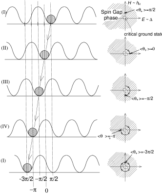
Figure 1: A sine curve represents the locking potential which slides adiabatically. As long as the sliding speed is low enough, the system (shaded circle) stays the same valley and does not jump into its neighboring valleys.

This relation always holds as far as the system is locked by the sliding potential $\sin(\hat{\theta}_{+}+\varphi(t))$, which is true for $|\gamma|\leq 1$.

Then we will argue the physical consequence of eq. (22). Generally speaking, when the bulk system has a finite spin gap, the effects of boundaries range over its magnetic correlation length from the both ends. Then we naturally divide the contribution to $P_{S^{z}}$ into following two parts;

$$P_{S^{z}} = P^{\rm{in}}_{S^{z}}+P^{\rm{edge}}_{S^{z}},\hskip 8.5359ptP^{\rm in(edge)}_{S^{z}}=\frac{1}{N}\sum_{j\in{\Omega_{\rm in(edge)}}}j\cdot\langle\hat{S}^{z}_{j}\rangle$$

where the $j$-summation in $P^{\rm{in}}_{S^{z}}$ are restricted within the interior of the systems ($\Omega_{\rm{in}}$), while spins within the edge region ($\Omega_{\rm{edge}}$) contribute to $P^{\rm{edge}}_{S^{z}}$. The “interior” of the system is defined as the region where the spin state is same as that of the periodic boundary condition (p.b.c.). Namely, the presence of the boundaries does not influence on the spin state of the interior. On the other hand, the spin state within the “edge” region is strongly affected by the boundaries. Then, by definition, the spins within the interior would turn back to the same spin configuration as that of the initial state after an adiabatic evolution along $\Gamma_{\rm{loop}}$,

$$\delta P^{\rm{in}}_{S^{z}}=0.$$

Therefore the difference of the spatial polarization of $\langle\hat{S}^{z}_{j}\rangle$ should be attributed to the change of spin configurations in the edge region,

$$\delta P^{\rm{edge}}_{S^{z}}=\frac{1}{N}\sum_{j\in{\Omega_{\rm{edge}}}}j\cdot\delta\langle\hat{S}^{z}_{j}\rangle=1.$$ (23)

In eq.(23), we next approximate $j$ for sites around the right end by $N/2$ and those of left by $-N/2$;

$$-\frac{1}{2}\sum_{j\simeq-\frac{N}{2}}\delta\langle S^{z}_{j}\rangle+\frac{1}{2}\sum_{j\simeq\frac{N}{2}}\delta\langle S^{z}_{j}\rangle\approx 1,$$ (24)

where we take the origin of site index $j$ at the center of the system. This approximation is allowed, since the edge region ranges over the magnetic correlation length from both ends, which is at most several sites in gapped spin systems. Thereby the semi-equal sign in eq.(24) could be safely replaced by the equal sign in the thermodynamic limit. When we bear in mind that the system has been staying on the eigenspace of $\hat{S}^{z}_{\rm{tot}}=0$ during this process;

$$\sum_{j\simeq-\frac{N}{2}}\delta\langle S^{z}_{j}\rangle+\sum_{j\simeq\frac{N}{2}}\delta\langle S^{z}_{j}\rangle=0,$$

eq.(24) indicates that the total $S^{z}$ around the right end ($j\simeq N/2$) increases by $1$ while that of the left end ($j\simeq-N/2$) decreases by $1$ along this cyclic evolution:

$$\sum_{j\in{\rm left\ end}}\delta\langle S^{z}_{j}\rangle=-1,\hskip 8.5359pt\sum_{j\in{\rm right\ end}}\delta\langle S^{z}_{j}\rangle=1.$$

Namely, the spin current quantized to $1$ flows from the left end of the system to the right end during this one cycle.

In summary, the quantized spin transport is always assured as long as $|\gamma|\leq 1$. This story does not alter even with the finite sliding speed $c=\frac{2\pi}{T}$, as far as it is slower than the height of this locking potential, in other words, the spin gap along the loop.

3 Numerical Analyses

In order to confirm the above argument, we performed the numerical calculation in the case of $|\gamma|=1$. Namely, we generated numerically the temporal evolution of the ground state wavefunction under the following time-dependent Hamiltonian:

$$|\phi(t)\rangle={\cal T}\Bigl{\{}\exp[{\rm i}\int_{0}^{t}{\rm d}t^{\prime}\hat{H}(t^{\prime})]\Bigr{\}}\cdot|g\rangle_{\rm{I}},$$

$$\hat{H}(t)=\sum_{i=1}^{N}\bigl{[}J-(-1)^{i}\Delta(t)\bigr{]}\mbox{\boldmath{$S$}}_{i}\cdot\mbox{\boldmath{$S$}}_{i+1}$$

$$\hskip 28.45274pt+\ h_{\rm{st}}(t)\sum_{i=1}^{N}(-1)^{i}S^{z}_{i},$$

$$(h_{\rm{st}}(t),\Delta(t))=R(\cos\frac{2\pi t}{T},\sin\frac{2\pi t}{T}),$$ (25)

where $\cal{T}$ represents the time order operator, $T$ is the cycle period during which the system has swept the loop ($\Gamma_{\rm{loop}}$) one time and $|g\rangle_{\rm{I}}$ is the ground state wavefunction at $(h_{\rm st},\Delta)=(R,0)$.

In Fig. 2, we show the expectation value of $\hat{S}^{z}_{j}$ taken over the final state, $|\phi(t=T)\rangle$, both with the p.b.c. and with the open boundary condition. The parameter $R$ is fixed to be $0.3$ and $J$ is taken as $1.5\ (0.6)$ in Fig. 2a(b). The cycle period $T$ is taken as 40 for the former and 80 for the latter, both of which are sufficiently long compared with the inverse of the spin gap observed along the loop.

Figure 2: (a): $\langle\hat{S}^{z}_{j}\rangle_{t=T}$ for $J=1.5,R=0.3$ and $T=40$, where $\delta P_{S^{z}}\equiv\langle\hat{P}_{S^{z}}\rangle_{t=T}-\langle\hat{P}_{S^{z}}\rangle_{t=0}=0.623$, (b): $\langle\hat{S}^{z}_{j}\rangle_{t=T}$ for $J=0.6,R=0.3$ and $T=80$, where $\delta P_{S^{z}}=0.862$.

For the p.b.c., as far as the sweeping velocity is low enough, the final state gives completely same configurations of $\langle\hat{S}^{z}_{j}\rangle$ as that of the initial antiferromagnetic ground state. However in the case of the o.b.c., the spins around both boundaries are clearly modified as seen in Fig. 2. When we read the total $S^{z}$ around the left end ( $\sum_{j=1}^{3}\langle\hat{S}^{z}_{j}\rangle$ ) and that of the right end ( $\sum_{j=12}^{14}\langle\hat{S}^{z}_{j}\rangle$ ) from Fig. 2a(b), the former increases by 0.67 (0.9) while the latter decreases by 0.67 (0.9) after this cyclic process. This result is qualitatively consistent with our preceding arguments.

In order to understand the difference between the result of the o.b.c. and that of the p.b.c., we also calculated the instantaneous eigenenergy as a function of $\varphi\equiv\frac{2\pi t}{T}$ in Fig. 3, where we take the offset as the ground state energy.

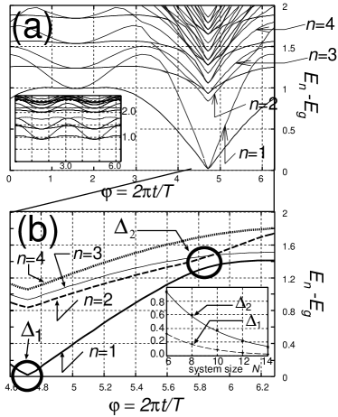
Figure 3: (a): Energy levels of all the eigenstates as a function of $\varphi\equiv\frac{2\pi t}{T}$ for the o.b.c. (inset: p.b.c.). $J=1.5$, $R=0.3$ and $N=14$. (b): Energy levels of those eigenstates with $\hat{S}^{z}_{\rm{tot}}=0$ for the o.b.c. $J=1.5$, $R=0.3$ and $N=14$. (inset: Size-dependence of the minimum energy gaps $\Delta_{1}\equiv{\rm{min}}_{\varphi}\bigl{[}E_{n=1}(\varphi)-E_{g}(\varphi)\bigr{]}$ and $\Delta_{2}\equiv{\rm{min}}_{\varphi}\bigl{[}E_{n=2}(\varphi)-E_{n=1}(\varphi)\bigr{]}$. Fitting curves for $\Delta_{1}$ and $\Delta_{2}$ are $0.32\exp(-(N-6)/3)$ and $0.925\exp(-(N-6)/4.3)$ respectively.)

For the p.b.c. (inset of Fig. 3a) , there is always a finite energy gap from the ground state for all $\varphi$. On the contrary, the gap for the o.b.c. reduces strongly at $\varphi=\frac{3\pi}{2}$ (Figs. 3a and 3b). Furthermore, this reduced energy gap $\Delta_{1}$ becomes smaller and smaller when we take the system size $N$ larger (inset of Fig. 3b, N=6,8,10,12), and the four states[39] including the ground state are nearly degenerate at $\varphi=\frac{3\pi}{2}$ for $N=14$.

Let us discuss the physical meanings of this quasi-degeneracy. At $(h_{\rm{st}},\Delta)=(0,-R)$, the exchange coupling between $\mbox{\boldmath{$S$}}_{2n}$ and $\mbox{\boldmath{$S$}}_{2n+1}$ ($n=1,2,...$) are strengthened (see eq.(25)) and dimers are formed between them, i.e.,

$$\mbox{\boldmath{$S$}}_{1}-\mbox{\boldmath{$S$}}_{2}=\mbox{\boldmath{$S$}}_{3}-\cdots-\mbox{\boldmath{$S$}}_{N-2}=\mbox{\boldmath{$S$}}_{N-1}-\mbox{\boldmath{$S$}}_{N}$$

where $\mbox{\boldmath{$S$}}_{i}=\mbox{\boldmath{$S$}}_{i+1}$ represents the singlet bond. Then, in the case of the o.b.c., the spin at $j=1$ and that of $j=N$ cannot form a spin singlet due to the absence of $\mbox{\boldmath{$S$}}_{1}\cdot\mbox{\boldmath{$S$}}_{N}$ term. Namely, in the limit of $J=R$, the following four states would be degenerated,

$$|\downarrow\rangle_{1}\otimes({\rm{dimer\ chain}})\otimes|\uparrow\rangle_{N},$$ (26)

$$|\uparrow\rangle_{1}\otimes({\rm{dimer\ chain}})\otimes|\downarrow\rangle_{N},$$ (27)

$$|\downarrow\rangle_{1}\otimes({\rm{dimer\ chain}})\otimes|\downarrow\rangle_{N},$$ (28)

$$|\uparrow\rangle_{1}\otimes({\rm{dimer\ chain}})\otimes|\uparrow\rangle_{N}.$$ (29)

The last two states ((28),(29)) do not belong to the eigenspace of $S^{z}_{\rm{tot}}=0$ and we ignore them henceforth.[39] When we introduce finite $J-R>0$, the $\frac{N}{2}$-th order perturbation in terms of $\hat{S}^{+}_{1}\hat{S}^{-}_{2}$, $\hat{S}^{+}_{3}\hat{S}^{-}_{4}$,…, and $\hat{S}^{+}_{N-1}\hat{S}^{-}_{N}$ (and their Hermite conjugate) lifts this degeneracy. Then the resulting gap should be scaled as $\exp(-N\alpha/l)$, where $l$ is expected to be a magnetic correlation length. In fact, we can fit the size dependence of $\Delta_{1}$ by this exponential function as in the inset of Fig. 3b, from which the correlation length at $\varphi=\frac{3\pi}{2}$ is estimated around $3$ sites. Because of this size dependence, we expect that $\Delta_{1}$ would vanish when we took the system size sufficiently large compared with this correlation length.

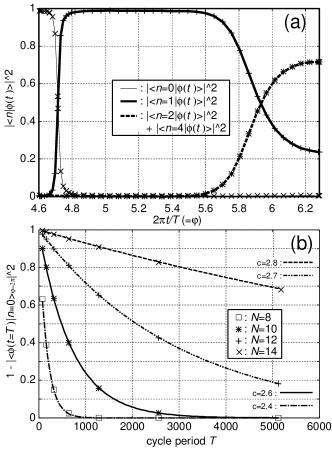
Figure 4: (a): Projected weight of $|\phi(t)\rangle$ onto each instantaneous eigenstate $|\langle n|\phi(t)\rangle|^{2}$ for $n=0,1,2,4$ where the w.f. $|\phi(t)\rangle$ is always almost perpendicular to the excited state with $n=3$: $|\langle n=3|\phi(t)\rangle|^{2}<10^{-7}$. $J=1.5$,$R=0.3$ and $N=14$. (b): Transition probability $P_{n=0\rightarrow n=1}$ as a function of cycle period $T$. Every data points are fitted by the Landau-Zener function $\exp\bigl{(}-\frac{\pi\Delta_{1}^{2}}{c\times 2\pi/T}\bigr{)}$, where $c$ is estimated around $2.5$. $J=1.5$ and $R=0.3$.

Because of this crossing character of the energy spectrum at $\varphi=\frac{3\pi}{2}$, the system which has resided on the ground state ($n=0$) transits, at $\varphi=\frac{3\pi}{2}$, into the first excited state with $n=1$ which is represented by the bold solid line in Fig. 3b. We can see this transition in Fig. 4a, where the projected weights of $|\phi(t)\rangle$ onto each instantaneous eigenstate are given as a function of $\varphi=\frac{2\pi t}{T}$. Futhermore, its transition probability, $P_{n=0\rightarrow n=1}$, is well fitted by the Landau-Zener formula[40, 41]

$$P_{n=0\rightarrow n=1}=\exp(-\frac{\pi\Delta_{1}^{2}}{c\times 2\pi/T}),$$

as in Fig. 4b, where we plotted $P_{n=0\rightarrow n=1}$ for various cycle period $T$ and various system size. From this fitting, $c$ in the Landau-Zener function is estimated around $2.6\pm 0.2$.[42]

As shown in the Fig. 4a, after the first transition took place at $\varphi=\frac{3\pi}{2}$, the second transition from the first excited state to the second excited state with $n=2$ (represented by the bold broken line) happens at $\varphi\simeq 5.9$. However its transition probability $P_{n=1\rightarrow n=2}$ is around $70\%$ and not so perfect compared with $P_{n=0\rightarrow n=1}$. This is mainly because the gap $\Delta_{2}$ around $\varphi\simeq 5.9$ between the first excited state and the second excited state is a substantial amount compared with $\Delta_{1}$ (see Fig. 3b). However, as in the inset of Fig. 3b, its size dependence is also scaled by

$$\Delta_{2}\sim{\rm exp}(-N\alpha/l),$$ (30)

where the magnetic correlation length $l$ is estimated around 4.6 sites. Therefore, when we take the system size large enough, we can naturally expect that the gap $\Delta_{2}$ would reduce exponentially, which enhances the transition probability $P_{n=1\rightarrow n=2}$ drastically.

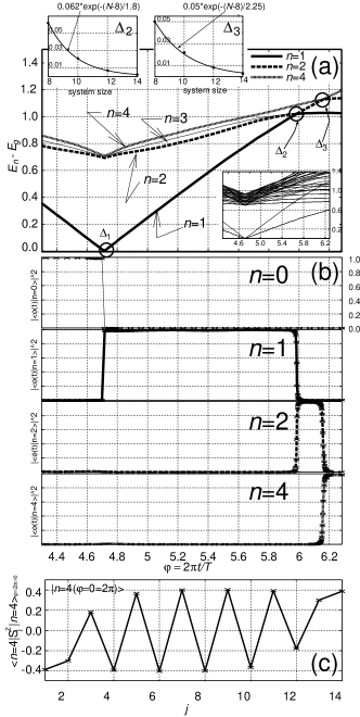
Figure 5: $J=0.6,R=0.3$ and $N=14$. (a): Energy spectrum for the eigenstates with $\hat{S}^{z}_{\rm{tot}}=0$ as a function of $\varphi$,(b): Projected weight of $|\phi(t)\rangle$ onto the lower five eigenstates, i.e., $|\langle\phi(t)|n\rangle|^{2}(n=0,1,2,4)$, (c): Expectation value of $\hat{S}^{z}_{j}$ taken over the fourth excited state with $n=4$ $|n=4\rangle_{\varphi=2\pi}$

In order to verify this expectation, we perform another numerical calculations. As it is very difficult to calculate numerically with larger system size ($N>14$), we, instead, decrease the ratio $J/R$ in order to reduce the magnetic correlation length $l$, which is also expected to reduce these gaps according to eq.(30). The result for $J=0.6,R=0.3$ and $N=14$ is summarized in Fig. 5. Figure5a indicates the energy spectrum for the lower four excited states with $\hat{S}^{z}_{\rm{tot}}=0$ and Fig. 5b shows the projected weight, $|\langle n|\phi(t)\rangle|^{2}$ for $n=0,1,2,4$. Figure5c represents the expectation value of $\hat{S}^{z}_{j}$ taken over the $|n=4\rangle_{\varphi=2\pi\equiv 0}$ as a function of site index $j$. Then, as is expected, the gaps we observed in Fig. 3 ($\Delta_{1},\Delta_{2}$) decrease drastically. In addition to them, there appears a new gap $\Delta_{3}$ between the excited state with $n=2$ and that with $n=4$ at $\varphi=6.15$. This gap $\Delta_{3}$ is also very tiny and scales as $\exp(-N/2.25)$.

As a result of these crossing characters of energy spectrum at $\varphi=\frac{3\pi}{2},5.97$ and $6.15$, three Landau-Zener type tunnelings take place as shown in Fig. 5b. Namely, the wavefunction $|\phi(t)\rangle$ changes its weight from the ground state with $n=0$ to the first excited state with $n=1$ (represented by the bold solid line in Fig. 5a) at $\varphi=\frac{3\pi}{2}$ , from the first excited state to the excited state with $n=2$ (bold broken line) at $\varphi=5.97$ and lastly from the excited state with $n=2$ to the fourth excited state with $n=4$ (bold dotted line) at $\varphi=6.15$. All these transition probabilities are almost $100\%$ in accordance with our previous expectations.[43]

After all, through these transitions, the wavefunction is raised from the ground state onto the fourth excited state ($n=4$) during this last quarter of the cycle. When we see the expectation value of $\hat{S}^{z}_{j}$ taken over this fourth excited state at $\varphi=0\equiv 2\pi$ (see Fig. 5c), it is almost identical to the solid line of the lower panel in Fig. 2, where the total $\hat{S}^{z}$ on the left end ($\sum_{j=1}^{3}\langle\hat{S}^{z}_{j}\rangle$) decreases by 0.9 while that of the right end ($\sum_{j=12}^{14}\langle\hat{S}^{z}_{j}\rangle$) increases by 0.9 in comparison with that of the initial ground state wavefunction.

To summarize, the numerical observations found in Fig. 2 can be ascribed to the difference between the energy spectrum with the p.b.c. and that with the o.b.c. In the latter case, a certain excited state decreases its energy level until $\varphi=\frac{3\pi}{2}$ and then picks up the system which has been staying on the ground state. Then, through the Landau-Zener tunnelings, several excited states carry the system hand in hand perfectly upon a particular excited state at $\varphi=0$, whose $\hat{P}_{S^{z}}$ increases by almost $1$ in comparison with that of the initial state. These observations remain unchanged if the sweeping velocity is always higher than $\frac{\pi\Delta^{2}_{i}}{c}$;

$$\frac{1}{T}>\max_{i=1,2,3}\Bigl{(}\frac{\pi\Delta^{2}_{i}}{c}\Bigr{)}.$$ (31)

This lower limit for the sweeping velocity is expected to vanish in the thermodynamic limit, since the $\Delta_{1,2,3}$ reduces exponentially to zero as the system size $N$ becomes larger. Therefore the conclusion in eq. (22) is consistent with the numerical results of this section.

Finally let us mention about the relevance of our story to real systems such as Cu-benzoate and ${\rm{Yb}}_{4}{\rm{As}}_{3}$. There the effective staggered field along the $z$-direction accompanies the uniform effective Zeeman fields along the $x$(or $y$)-direction, $H^{x(y)}_{u}$. Furthermore, since these systems break the bond-centered inversion symmetry, there is a Dzyaloshinskii-Moriya (DM) interaction. Its DM vector must alternate bond by bond in the absence of the electric field. In addition to them, the uniform component of the DM vector would be also induced by the applied electric field in general. Even if these terms are gradually introduced to our model calculations, $\delta\theta_{+}$ remains invariant as far as the gap along the loop remains open, in other words, the system along the loop remains locked by the sliding potential $\sin(\hat{\theta}_{+}+\varphi(t))$. This is a manifestation of the fact that the quantized $\delta\theta_{+}$ (in the thermodynamic limit) is a topologically protected quantity. However, detail studies on the effect of these terms might be remaining interesting problems.

When the system travels around this critical ground state $M$ times, total $z$-component of spin around one end increases by $M$, while that on the other end decreases by a same amount. Such an inhomogeneous magnetic structure can be detectable around sample boundaries and/or magnetic domain boundaries by using some optical probes. However, we must mention that the excited state with $P_{S^{z}}=m$ (In the case of $m=1$, this corresponds to $|n=4\rangle_{\varphi=0}$ in Fig. 5) might fall into the ground state $|n=0\rangle_{\varphi=0}$ by way of the $x$-component of the uniform magnetic field $H^{x}_{\rm{u}}$ at around $t=mT$, when we sweep the system slower than $2\mu_{B}H^{x}_{\rm u}$. In order to avoid this relaxation process, the sweeping velocity should be taken faster than $2\mu_{B}H^{x}_{\rm{u}}$.

$$\frac{1}{T}>2\mu_{B}H^{x}_{\rm u},$$ (32)

However, in order to keep the system on a particular minimum of the locking potential $\cos(\theta_{+}+\frac{2\pi t}{T})$, the velocity must be also slower than the spin gap observed along the loop,

$$\frac{1}{T}<J^{1/3}R^{2/3}.$$ (33)

Therefore we need to have a finite window between the lower limit of the sweeping velocity and the upper limit. In the case of Cu-benzoate, the spin gap of $0.1\rm{meV}$ is induced by the applied magnetic field of $1\rm{T}$ $(2\mu_{B}\times 1{\rm T}\sim 0.1\rm{meV})$. Thereby, the lower limit of this sweeping velocity is unhappily comparable to the higher limit in this system. However, spin gaps around $0.1\rm{meV}$ could be also induced by the magnetic field smaller than $1\rm{T}$ in those quantum spin chains with relatively larger $J$, where substantial amount of the window between the upper limit and the lower limit would exist. Therefore, it is not so hard to realize our story experimentally on the quasi-1D quantum spin systems with relatively large intrachain interaction and with two crystallographically inequivalent sites in its unit cell.

We also want to mention about the magnitude of the electric field required in order to induce the dimerization gap enough to be observable and also enough to be comparable to the spin gap induced by the magnetic field, which is around $0.1{\rm{meV}}$. Since it goes beyond the scope of this paper to quantify microscopically the change of the exchange interaction induced by external electric fields, we will pick up some reference data from other materials. Let’s see magneto-electric materials, where the applied electric field often changes its effective exchange interactions $J$ due to its peculiar crystal structure and its change $\Delta$ could be quantitatively estimated via the resulting magnetization. [45] In the case of famous magneto-electric material ${\rm{Cr}}_{2}{\rm{O}}_{3}$, the intra-sublattice exchange interaction for the + sublattice and that for the $-$ sublattice should be equal to each other because of the inversion symmetry ($J_{+}=J_{-}=J$). Then an electric field applied along its principle axis breaks this symmetry and induce a finite difference $\Delta=J_{+}-J_{-}$, where $\Delta/J$ was estimated around $10^{-5}$ under $E\sim 1{\rm{kV/cm}}$.[45] Namely,

$$\frac{\Delta}{J}=cE.$$ (34)

with its linear coefficient $10^{-5}[{\rm cm/kV}]$. When we apply this coefficient to our Heisenberg model, eq.(2) with $J\sim 0.1\rm{eV}$, we need an electric field of order of $1{\rm{kV/cm}}$ in order to induce the dimerizing gap $J^{1/3}\Delta^{2/3}$ of order of $0.1\rm{meV}$, which is still one order of magnitude smaller than the typical value of the Zener’s breakdown field ($\geq 10^{4}\rm{V/cm}$ at $T\leq 100{\rm K}$) of $1$D Mott insulators.[46]

4 Conclusion and discussion

In this paper, we propose the quantum spin pumping in $S=1/2$ quantum spin chains with two crystallographically inequivalent sublattices in its unit cell ($T,I_{\rm{bond}}$ : broken and $I_{\rm{site}}$ : unbroken) and with relatively large intrachain exchange interactions. Due to its peculiar crystal structure, an applied electric field ($E$) and magnetic field ($H$) endow its critical ground state with the finite spin gap via the dimerizing field ($\Delta\sim E$) and the staggered magnetic field ($h_{\rm{st}}\sim H$), respectively, where the phase operator $\hat{\theta}_{+}$ in sine-Gordon theory is locked on a particular valley of the relevant potential $\sqrt{h_{\rm{st}}^{2}+\Delta^{2}}\sin(\hat{\theta}_{+}+\varphi)$ : $\langle\hat{\theta}_{+}\rangle=\frac{\pi}{2}-\varphi+2\pi n$. When the system is deformed slowly along the loop which encloses the critical ground state in the $E$-$H$ plane, the locking potential $\sqrt{h_{\rm{st}}^{2}+\Delta^{2}}\sin(\hat{\theta}_{+}+\varphi)$ in the sine-Gordon model slides gradually (see Fig. 1). After one cycle along this loop, the expectation value of the phase operator $\hat{\theta}_{+}$ for the ground state acquires $2\pi$ holonomy. This means that a spatial polarization of $z$-component of spins $P_{S^{z}}$ increases by $1$ after this cycle [56]. In other words, the $z$-component of the spin current quantized to be $1$ flows through the bulk system during this cycle.

These arguments are supported by the numerical analyses, where we performed the exact diagonalization of the finite size system and developed the ground state wavefunction along this loop in a thermally insulating way.

Appendix A Equivalence between the phase operator and the spatial polarization operator

In this appendix, we will show that the continuum limit of $\hat{P}_{S^{z}}$ corresponds to the phase operator $-\frac{1}{N\alpha}\int\frac{\hat{\theta}_{+}(y)}{2\pi}{\rm d}y$, where related work was done by Nakamura and Voit.[47] Historically the polarization operator is known to be an ill-defined operator on the Hilbert space with the periodic boundary condition (p.b.c.) and is consequently formidable to treat in solid state physics. However, recently King-Smith and Vanderbilt[51, 52] and Resta[48, 49, 50, 53] showed that the derivative of the polarization with respect to some external parameter $\lambda$ can be expressed by the current operator which is in turn well-defined in the Hilbert space with the p.b.c.. Based on this observation, they quantitatively estimated electronic contributions to macroscopic polarizations in dielectrics and semiconductors such as GaAs, ${\rm{KNbO}}_{3}$ and III-V nitride. Following their strategies, we will show the equivalence between the derivative of $-\frac{1}{N\alpha}\int{\rm d}y\langle\frac{\hat{\theta}_{+}(y)}{2\pi}\rangle$ with respect to $\lambda$ and that of $\langle P_{S^{z}}\rangle$.

According to the standard perturbation theory[49], the derivative of the polarization with respect to some mechanical parameter $\lambda$ is given by

$$\frac{\partial\langle\hat{P}_{S^{z}}\rangle}{\partial\lambda}=-\sum_{N\neq g}$$

$$\Bigl{[}\frac{\langle g(\lambda)|[{\hat{P}_{S^{z}}},\hat{H}]|N(\lambda)\rangle\langle N(\lambda)|\frac{\partial\hat{H}(\lambda)}{\partial\lambda}|g(\lambda)\rangle}{(E_{g}(\lambda)-E_{N}(\lambda))^{2}}+{\rm{c.c.}}\Bigr{]},$$ (35)

where we assume the system has a finite spin gap from the ground state. The time derivative of $P_{S^{z}}$ in the numerator reduces to the summation of the current operator over all bonds;

$$-{\rm i}\Bigl{[}{\hat{P}_{S^{z}}},H\Bigr{]}=-{\rm i}\Bigl{[}{\hat{P}_{S^{z}}},H_{\rm XY}+H_{\rm dim}\Bigr{]}$$

$$={\rm i}\frac{1}{N}\sum_{j=1}^{N}\sum_{k=1}^{N-1}\Bigl{[}j\hat{S}^{z}_{j},-\frac{1}{2}\bigl{[}J+(-1)^{k}\Delta\bigr{]}(\hat{S}^{+}_{k}\hat{S}^{-}_{k+1}+{\rm{c.c.}})\Bigr{]}$$

$$=\frac{\rm i}{2N}\sum_{j=1}^{N-1}\bigl{[}J+(-1)^{j}\Delta\bigr{]}(\hat{S}^{-}_{j}\hat{S}^{+}_{j+1}-\hat{S}^{+}_{j}\hat{S}^{-}_{j+1}).$$ (36)

Thereby the contribution of every single bond is always ${\cal{O}}(1/N)$, which is not the case with $\hat{P}_{S^{z}}=\frac{1}{N}\sum_{j=1}^{N}j\hat{S}^{z}_{j}$. As a result, we are allowed to estimate with the periodic boundary condition the r.h.s. of eq. (36) in the thermodynamic limit, which we should have figured out with the open boundary. This is because their difference is attributed to the spin currents on the several bonds[54] around the boundaries, which is at most ${\cal{O}}(1/N)$ in our spin gapped system. Then we will consider eq. (36) with the p.b.c. and rewrite it in terms of the bosonization language. That is to say, we express the current operator in eq. (36) in terms of the phase operator $\hat{\theta}_{+}(x)$ and its conjugate field $\hat{\Pi}(x)$,

$$\hat{S}^{+}_{j+1}\hat{S}^{-}_{j}-\hat{S}^{+}_{j}\hat{S}^{-}_{j+1}=f^{\dagger}_{j+1}f_{j}-f^{\dagger}_{j}f_{j+1}$$

$$\approx\ \Bigl{[}R^{\dagger}(x_{j+1})e^{-{\rm i}k_{F}x_{j+1}}+L^{\dagger}(x_{j+1})e^{{\rm i}k_{F}x_{j+1}}\Bigr{]}$$

$$\hskip 14.22636pt\times\ \Bigl{[}R(x_{j})e^{{\rm i}k_{F}x_{j}}+L(x_{j})e^{-{\rm i}k_{F}x_{j}}\Bigr{]}-{\rm H.c.}$$

$$\approx\ -2{\rm i}\cdot\Bigl{[}R^{\dagger}(x_{j})R(x_{j})-L^{\dagger}(x_{j})L(x_{j})\Bigr{]}$$

$$+\ {\rm i}\alpha\cdot(-1)^{j}\Bigl{[}R^{\dagger}(x_{j}){\partial_{x}}L(x_{j})-L^{\dagger}(x_{j}){\partial_{x}}R(x_{j})+{\rm{H.c.}}\Bigr{]}$$

$$=\ 4{\rm i}\hat{\Pi}(x_{j})$$

$$\ \ +\ {\rm i}(-1)^{j}\Bigl{[}2\hat{\Pi}(x_{j})\cos\hat{\theta}_{+}(x_{j})+{\rm H.c.}\Bigr{]}.$$ (37)

Accordingly, the time derivative of $P_{S^{z}}$ in the continuum limit can be expressed in the following form,

$$-{\rm i}\Bigl{[}{\hat{P}_{S^{z}}},H\Bigr{]}$$

$$\approx-\frac{1}{N\alpha}\int{\rm d}x\biggl{\{}2J\hat{\Pi}+\Delta\Bigl{[}\hat{\Pi}\cos\hat{\theta}_{+}+{\rm H.c.}\Bigr{]}\biggr{\}}.$$ (38)

From now on, we will show that this expression is identical to the time derivative of the phase operator:

$$\mbox{(r.h.s. of eq.(\ref{3-2}))}={\rm i}[\frac{1}{N\alpha}\int{\rm d}x\frac{\hat{\theta}_{+}(x)}{2\pi},\hat{H}].$$ (39)

The first term in the r.h.s. of eq.(38) comes from the commutator between $\hat{\theta}_{+}$ and $H_{\rm XY}$ given in eq.(16),

$${\rm i}\Bigl{[}\frac{\hat{\theta}_{+}(x)}{2\pi},H_{\rm{XY}}\Bigr{]}=-2J\hat{\Pi}(x).$$ (40)

On the other hand, the commutator between the phase operator and $H_{\rm dim}$ given in eq.(18) vanishes and does not produce the last two terms of eq. (38). This is because eq.(18) is not an accurate expression for $H_{\rm dim}$ in the continuum limit and needs some additional terms, whose commutators with the phase operator correctly yield the last two terms of eq. (38). In order to prove that this is indeed the case, we will carefully reexamine the bosonization of $\hat{S}^{+}_{j}\hat{S}^{-}_{j+1}+\hat{S}^{+}_{j+1}\hat{S}^{-}_{j}$ [55] :

$$\hat{S}^{+}_{j}\hat{S}^{-}_{j+1}+{\rm H.c.}$$

$$=\ \Bigl{[}R^{\dagger}(x_{j})e^{-{\rm i}k_{F}x_{j}}+L^{\dagger}(x_{j})e^{{\rm i}k_{F}x_{j}}\Bigr{]}$$

$$\hskip 14.22636pt\times\ \Bigl{[}R(x_{j+1})e^{{\rm i}k_{F}x_{j+1}}+L(x_{j+1})e^{-{\rm i}k_{F}x_{j+1}}\Bigr{]}+{\rm H.c.}$$

$$\approx\ ({\rm{r.h.s}}\ \ {\rm{of}}\ \ {\rm{eq.(\ref{1-1-2})}})-{\rm i}(-1)^{j}\frac{\alpha^{2}}{2}\cdot\Bigl{[}R^{\dagger}(x_{j}){\partial_{x}}^{2}L(x_{j})$$

$$\ \ \ -L^{\dagger}(x_{j}){\partial_{x}}^{2}R(x_{j})-{\rm H.c.}\Bigr{]}$$

$$=\mbox{ (r.h.s. of eq. (\ref{2-0-2}))}$$

$$\hskip 14.22636pt+\ (-1)^{j}\alpha\biggl{\{}-\frac{1}{4\pi}(\partial_{x}\hat{\theta}_{+}(x_{j}))^{2}\cos\hat{\theta}_{+}(x_{j})$$

$$\hskip 14.22636pt+\ \pi\Bigl{[}\hat{\Pi}^{2}(x_{j})\cdot\cos\hat{\theta}_{+}(x_{j})$$

$$\hskip 14.22636pt+\ \hat{\Pi}(x_{j})\cdot\cos\hat{\theta}_{+}(x_{j})\cdot\hat{\Pi}(x_{j})+{\rm{H.c.}}\Bigr{]}\biggr{\}}.$$ (41)

Then, by taking its staggered components, we obtain the following expression for $H_{\rm dim}$, instead of eq.(18),

$$H_{\rm{dim}}=$$

$$\Delta\int{\rm d}x\Biggl{\{}-\frac{1}{\pi\alpha^{2}}\cos\hat{\theta}_{+}-\frac{1}{8\pi}\left(\partial_{x}\hat{\theta}_{+}\right)^{2}\cos\hat{\theta}_{+}$$

$$+\ \frac{\pi}{2}\biggl{[}\hat{\Pi}^{2}\cdot\cos\hat{\theta}_{+}+\hat{\Pi}\cdot\cos\hat{\theta}_{+}\cdot\hat{\Pi}+{\rm{H.c.}}\biggr{]}\Biggr{\}}.$$ (42)

Here we want to mention that, irrespective of this modification, $\cos\hat{\theta}_{+}$ in $H_{\rm dim}$ always locks the phase operator in combination with $\sin\hat{\theta}_{+}$ in $h_{\rm st}$ as far as $|\gamma|\leq 1$ (see the text). This is because the RG eigenvalues of the additional terms such as $(\partial_{x}\hat{\theta}_{+})^{2}\cos\hat{\theta}_{+}$, $(\hat{\Pi})^{2}\cos\hat{\theta}_{+}$ and etc. are all negative and thereby irrelevant in the sense of the renormalization group study. However these additional terms in $H_{\rm dim}$ cannot be discarded, since the commutator between these terms and the phase operator produces the last two term of eq.(38):

$${\rm i}\bigl{[}\frac{\hat{\theta}_{+}(x)}{2\pi},H_{\rm dim}\bigr{]}$$

$$=\ -\Delta\biggl{[}\hat{\Pi}(x)\cos\hat{\theta}_{+}(x)+\cos\hat{\theta}_{+}(x)\hat{\Pi}(x)\biggr{]}.$$ (43)

After all, by comparing eqs.(40) and (43) with eq.(38), we can safely replace $-i[P_{S^{z}},H]$ by $\frac{i}{N\alpha}\int{\rm d}x[\frac{\hat{\theta}_{+}}{2\pi},H]$ in the continuum limit and rewrite eq. (35) into a following simple form by using the bosonization language:

$$\frac{\partial\langle\hat{P}_{S^{z}}\rangle}{\partial\lambda} \approx \frac{1}{N\alpha}\sum_{N\neq g}\int{\rm d}x\Biggl{[}\frac{\langle g|[\frac{\hat{\theta}_{+}(x)}{2\pi},\hat{H}]|N\rangle\langle N|\frac{\partial\hat{H}}{\partial\lambda}|g\rangle}{(E_{g}-E_{N})^{2}}+{\rm{c.c.}}\Biggr{]}$$ (44)

$$= -\frac{1}{N\alpha}\sum_{N}\int{\rm d}x\Bigl{[}\langle g|\frac{\hat{\theta}_{+}(x)}{2\pi}|N\rangle\langle N|\frac{\partial}{\partial\lambda}|g\rangle+{\rm{c.c.}}\Bigr{]}$$

$$= -\frac{1}{N\alpha}\int{\rm d}x\frac{\partial}{\partial\lambda}\langle\frac{\hat{\theta}_{+}(x)}{2\pi}\rangle.$$

Here we used $\langle N|\frac{\partial\hat{H}}{\partial\lambda}|g\rangle=(E_{g}-E_{N})\langle N|\frac{\partial}{\partial\lambda}|g\rangle$.

References

- [1] Y.Tokura et al.: Colossal Magnetoresistive Oxides(Taylor Francis, London, 2000)
- [2] R. Karplus and J. M. Luttinger: Phys. Rev. 95 (1954) 1154.
- [3] J. Smit: Physica 21, 877 (1955); 24 (1958) 39
- [4] P. Nozires and C. Lewiner: J. Phys. (Paris) 34 (1973) 901
- [5] J. Kondo: Prog. Theor. Phys. 27 (1963) 772
- [6] P. Matl, N. P. Ong, Y. F. Yan, Y. Q. Li , D. Studebaker, T. Baum, and G. Doubinina: Phys. Rev. B 57 (1998) 10248
- [7] S. H. Chun, M. B. Salamon, Y. Lyanda-Geller, P. M. Goldbart, and P. D. Han: Phys. Rev. Lett. 84 (2000) 757
- [8] J. Ye, Y. B. Kim, A. J. Millis, B. I. Shraiman, P. Majumdar, and Z. Teanovi: Phys. Rev. Lett. 83 (1999) 3737
- [9] K. Ohgushi, S. Murakami and N. Nagaosa: Phys. Rev. B 62 (2000) R6065
- [10] Y. Taguchi, Y. Oohara, H. Yoshizawa, N. Nagaosa, Y. Tokura: Science 291 (2001) 2573; Y. Taguchi,T. Sasaki,S. Awaji, Y. Iwasa, T. Tayama, T. Sakakibara , S. Iguchi, T. Ito and Y. Tokura: Phys. Rev. Lett. 90 (2003) 257202
- [11] T. Kageyama, S. Iikubo, S. Yoshii, Y. Kondo, M. Sato and Y. Iye: J. Phys. Soc. Jpn. 70 (2001) 3006
- [12] S. Onoda and N. Nagaosa: Phys. Rev. Lett. 90 (2003) 196602
- [13] R. Shindou and N. Nagaosa: Phys. Rev. Lett. 87 (2001) 116801
- [14] G. Tatara and H. Kawamura: J. Phys. Soc. Jpn. 71 (2002) 2613
- [15] H. Kawamura: Phys. Rev. Lett. 90 (2003) 047202
- [16] M. Onoda and N. Nagaosa: J. Phys. Soc. Jpn. 71 (2002) 19 ; Phys. Rev. Lett. 90 (2003) 206601
- [17] T. Jungwirth, Q. Niu and A. H. MacDonald: Phys. Rev. Lett. 88 (2002) 207208; T. Jungwirth, J. Sinova, K. Y. Wang, K. W. Edmonds, R. P. Campion, B. L. Gallagher, C. T. Foxon, Q. Niu and A. H. MacDonald: Appl. Phys. Lett. 83 (2003) 320
- [18] A. A. Burkov and L. Balents: Phys. Rev. Lett. 91 (2003) 057202
- [19] Z. Fang, N. Nagaosa, K. S. Takahashi, A. Asamitsu, R. Mathieu, T. Ogasawara, H. Yamada, M. Kawasaki and Y. Tokura: Science 302 (2003) 92
- [20] Y. Yao, L. Kleinman, A. H. MacDonald, S. Sinova, D. Wang, E. Wang and Q. Niu: Phys. Rev. Lett. 92 (2004) 037204
- [21] D. J. Thouless: Phys. Rev. B 27 (1983) 6083
- [22] Q. Niu and D. J. Thouless: J. Phys. A 17 (1984) 2453
- [23] B. L. Altshuler, L. I. Glazman, Science 283 (1999) 1864
- [24] M. Switkes, C. M. Marcus, K. Campman and A. C. Gossard: Science 283 (1999) 1905
- [25] J. M. Shilton,V. I. Talyanskii, M. Pepper, D. A. Ritchie, J. E. F. Frost, C. J. B. Ford, C. G. Smith, and G. A. C. Jones: J. Phys. Condens. Matter 8 (1996) L531
- [26] V. I. Talyanskii, J. M. Shilton, M. Pepper,C. G. Smith, C. J. B. Ford, E. H. Linfield, D. A. Ritchie, and G. A. C. Jones: Phys. Rev. B 56 (1997) 15180
- [27] Hamiltonian has also a staggered Dzyaloshinskii-Moriya vector, whose effect can be renormalized into the staggered -tensor . When the system is invariant under the -rotational symmetry which exchanges nearest neighbor sites, bare becomes a non-generic matrix in general.
- [28] D. C. Dender, P. R. Hammar, D. H. Reich, C. Broholm and G. Aeppli: Phys. Rev. Lett. 79 (1997) 1750
- [29] M. Oshikawa and I. Affleck: Phys. Rev. Lett. 79 (1997) 2883; I. Affleck and M. Oshikawa: Phys. Rev. B 60 (1999) 1038. In these papers, not only the staggered component of -tensor but also the alternating DM vector are found to be relevant to induce a finite spin gap.
- [30] M. Oshikawa, K. Ueda, H. Aoki, A. Ochiai and M. Kohgi: J. Phys. Soc. Jpn. 68 (1999) 3181
- [31] If the system is invariant under the -rotational symmetry which exchanges the nearest neighboring bonds , the direction of must be deviated from this -rotational axis.
-
[32]
Here we also rotate by around the -direction
in the spin space on odd sites:
We take this sign convention only in 2.(45) - [33] P. Jordan and E. Wigner: Z.Phys. 47 (1928) 631
- [34] E. Lieb, T. Schultz, and D. C. Mattis: Ann. Phys. (N.Y.) 16 (1961) 407
- [35] J. E. Avron, A. Raveh and B. Zur: Rev. Mod. Phys. 60 (1988) 873;J. E. Avron, J. Berger and Y. Last: Phys. Rev. Lett. 78 (1997) 511
- [36] N. Nagaosa: Quantum Field Theory in Strongly Correlated Electronic Systems (Springer, Berlin, 1999)
-
[37]
For example, R. Shankar: Acta Phys. Pol. B 26 (1995) 1835.
From this paper, we change its notations as follows;
, - [38] S.Eggert and I.Affleck, Phys. Rev. B 46 (1992) 10866
- [39] The energy level which reaches around 0.9 at in Fig.3a corresponds to doubly degenerate eigenstates which belong to the eigenspaces of respectively. These doubly degenerate states at corresponds to the two state given in eqs. (28) and (29). On the contrary, the eigenstate labeled as (represented by the bold solid line in Fig. 3b) and the ground state belong to the eigenspace of . Since our time-dependent Hamiltonian conserves the total spin density , does not have projected weights onto those eigenstates with .
- [40] C. Zener: Proc. R. Soc. London, Ser. A137 (1932) 696
- [41] S. Miyashita: J. Phys. Soc. Jpn. 64 (1994) 3207
- [42] We identify as .
- [43] Here the wavefunction does not have the projected weight on the third excited state with (thin line in Fig. 5a) during the cycle.
- [44] The uniform component of the Zeeman field does not cause the spin gap to the critical ground state of the isotropic Heisenberg model as far as it is small. In contrast the staggered component is always relevant even if it is infinitesimally small. However when the uniform component of the magnetic field is very strong, the system will be governed by the fixed point where the ground state is ferromagnetically polarized with a finite spin gap. This fixed point is different from the fixed point at which the system is locked by the staggered component of the magnetic field, i.e., . As far as the system under the applied magnetic field is governed by the latter fixed point, is quantized to be .
- [45] R. Hornreich and S. Shtrikman: Phys. Rev. 161 (1967) 506; K. Shiratori and E. Kita: Kotai-Butsuri 14 (1979) 599 (in Japanese)
- [46] Y. Taguchi, T. Matsumoto and Y. Tokura: Phys. Rev. B 62 (2000) 7015
- [47] M. Nakamura and J. Voit: Phys. Rev. B 65 (2002) 153110; M. Nakamura and S. Todo: Phys. Rev. Lett. 89 (2002) 077204. In these papers, -operator introduced by R.Resta and Sorella[50], Aligia and Ortiz[53] is applied to the quantum spin systems and is used to distinguish various spin gap phases.
- [48] R. Resta: Ferroelectrics 22 (1993) 133; R. Resta, M. Posternak and A. Baldereschi: Phys. Rev. Lett. 70 (1993) 1010; ibid. Phys. Rev. B 50 (1994) 8911.
- [49] R. Resta: Rev. Mod. Phys. 55 (1994) 899
- [50] R. Resta: Phys. Rev. Lett. 80 (1998) 1800; R. Resta and S. Sorella: Phys. Rev. Lett. 82 (1999) 370
- [51] R. D. King-Smith and D. Vanderbilt: Phys. Rev. B 47 (1993) 1651; D. Vanderbilt and R. D. King-Smith: Phys. Rev. B 48 (1993) 4442; F. Bernardini, V. Fiorentini and D. Vanderbilt: Phys. Rev. B 56 (1997) 10024
- [52] G. Ortiz and R. M. Martin: Phys. Rev. B 49 (1994) 14202
- [53] A. A. Aligia and G. Ortiz: Phys. Rev. Lett.82 (1999) 2560
- [54] In spin-gapped systems, the effects of the boundary range only within its magnetic correlation length from both ends.
- [55] In the final line of eq.(41), we drop those terms which can be summarized into a form of the total derivative.
- [56] P. Sharma and C. Chamon: Phys. Rev. Lett. 87 (2001) 096401; ibid. Phys. Rev. B 68 (2003) 035321. Similar arguments as we have employed in 2 are also found in this work, where one-dimensional Luttinger liquid (LL) between two separated contacts reduces to two decoupled LL wires due to the back scattering potential in between. Namely, the spin part of their back scattering potential is also described by , where denotes the phase operator at the midpoint of two contacts. This backscattering potential turns out to be relevant in the presence of repulsive electron-electron interactions and tunneling probability of spins between two contacts becomes vanishing. As a consequence of this vanishing tunneling probability of spins (TPS), number of spins transported between these two contacts is also quantized in their work. Even though our work treats a pumping in macro-scale systems and is different from their work which is about meso (nano)-scale systems, there is an interesting correspondence between these two works. Namely, in both stories, quantizations of spin transports result from the vanishing TPS between two “contacts”. Two contacts in their configurations correspond to the two sample boundaries in this paper and TPS between these two “contacts”, namely tunneling probability between the state of eq.(26) and that of eq.(27) decreases exponetially in thermodynamic limit, which is also a necessity of the quantized spin transfers in this paper (see 3).