Horizontal line nodes in superconducting Sr₂RuO₄

Abstract

We analyze the possibilities of triplet pairing in Sr₂RuO₄ based upon an idea of interlayer coupling. We have considered two models differing by the effective interactions. In one model the quasi-particle spectra have horizontal line nodes on all three Fermi surface sheets, while in the other the spectra have line or point nodes on the $\alpha$ and $\beta$ sheets and no nodes on the $\gamma$ sheet. Both models reproduce the experimental heat capacity and penetration depth results, but the calculated specific heat is sightly closer to experiment in the second solution with nodes only on the $\alpha$ and $\beta$ sheets.

Subject classification:74.70.Pq,74.20.Rp,74.25.Bt

1 1. Introduction.

Strontium Ruthenate (Sr₂RuO₄) is widely believed to be a spin triplet superconductor[1, 2, 3, 4], however the theoretical model and particular pairing mechanism are still hotly debated [5, 6, 7, 8, 9, 10, 11, 12, 13]. Its lattice structure resembles the layered structure of the cuprate La_2-xBa_xCuO₄ but, instead of high temperature d-wave superconductivity, the superconducting phase of strontium ruthenate ($T_{c}\sim 1.5$K) appears to be p-wave or f-wave in nature. The strongest evidence for this comes from the ¹⁷O NMR Knight shift data[14] and neutron scattering experiments[15] which indicate that the in-plane Pauli spin susceptibility is constant below $T_{c}$. These experiments could be naturally explained with a triplet pairing state ${\bf d}(\bf k)={\bf e}_{z}(k_{x}\pm ik_{y})$ in exact analogy with the ABM phase of superfluid ³He. The $\mu$SR experiments[16] also indicate a spontaneous breaking of time reversal symmetry at $T_{c}$, which would be consistent with such a chiral ABM type state. On the other hand several experiments[17, 18, 19] indicate that the gap function must have lines of nodes on the Fermi surface, unlike the simple ABM state which is nodeless on the three cylindrical sheets, $\alpha$, $\beta$ and $\gamma$, of the Fermi surface of Sr₂RuO₄.

In this paper we address the question of the possible location of these line nodes on the Fermi surface. We concentrate on the case of horizontal lines of nodes, because vertical nodes (for example in f-wave pairing states) appear to be inconsistent with the absence of angular dependence of the thermal conductivity in an a-b plane magnetic field[19, 20]. The presence of horizontal lines of nodes, as originally suggested by Hasegawa, Machida and Ohmi[5], cannot be explained in any 2-d theoretical model but requires a 3-d model with at least some component of the pairing interaction acting between planes. A number of such models assuming interlayer coupling have been proposed[6, 7, 8, 9, 10, 11, 12, 13].

The specific question which we address here is whether there are horizontal line nodes on all three Fermi surface sheets, as proposed recently by Koikegami, Yoshida and Yanagisawa[11], or whether the nodes are only on the $\alpha$ and $\beta$ sheets, as proposed by Zhitomirsky and Rice[8] and in our earlier interlayer coupling model[9, 10, 12]. To answer this question we will analyze, an effective week coupling model where the attractive interactions can appear between electrons on nearest neighbour and next nearest neighbour lattice sites (symbolised by 2 and 3 lines in Fig. 1). We will contrast the predictions of our original interlayer coupling model[9, 10, 12] with ones chosen to reproduce the gap structure proposed by Koikegami, Yoshida and Yanagisawa[11].

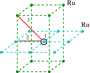
Figure 1: Body-centred tetragonal lattice of Ruthenium atoms in the Sr₂RuO₄ structure. The full lines show possible interactions between electrons occupying the single site ’1’ and its in-plane nearest neighbour sites ’2’ and intra-plane neighbours ’3’.

Figure 2: Orientation of $d_{xz}$ and $d_{yz}$ and $d_{xy}$ orbitals.

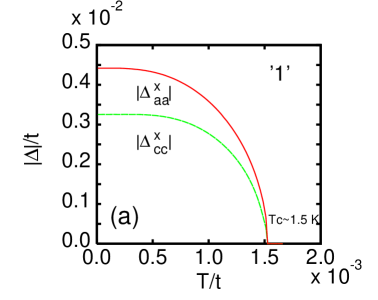
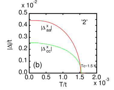
Figure 3: Temperature dependence of order parameters $\Delta_{aa}^{\perp,x}$, $\Delta_{cc}^{\perp,x}$ (a) and $\Delta_{aa}^{\perp,x}$ and $\Delta_{cc}^{\parallel,x}$ (b) found for different choice of interactions. Fig. 3a corresponds to the results for only $U^{\perp}_{m,m^{\prime}}(ij)<0$ (Eq. 2 - scenario 1) while Fig. 3b to the case where $U^{\perp}_{m,m^{\prime}}(ij)<0$ for $m,m^{\prime}=a,b$ (Eq. 3 - scenario 2) and $U^{\parallel}_{c,c}(ij)<0$.

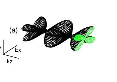
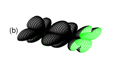
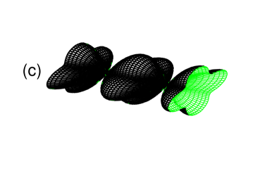
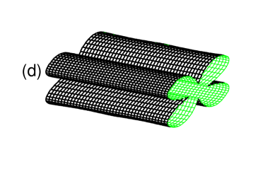
Figure 4: Minimum energy quasiparticle eigenvalues on the $\alpha$ (a) , $\beta$ (b) and $\gamma$ (c,d) Fermi surface sheets. Fig. 4c (scenario 1) corresponds to the results for only $U^{\perp}_{m,m^{\prime}}(ij)<0$ while Fig. 4d (scenario 2) to the case where $U^{\perp}_{m,m^{\prime}}(ij)<0$ for $m,m^{\prime}=a,b$ and $U^{\parallel}_{c,c}(ij)<0$. Fig. 4a and b are the same for both cases.

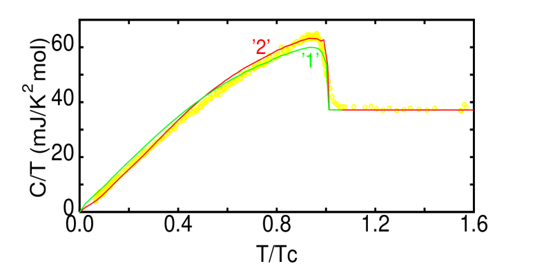
Figure 5: Calculated specific heat, $C$, as a function of temperature, $T$, compared to the experimental data of NishiZaki et al.[17] (gray circles). The line ’1’ shows the results for only $U^{\perp}_{m,m^{\prime}}(ij)<0$ while line ’2’ corresponds to the case where $U^{\perp}_{m,m^{\prime}}(ij)<0$ for $m,m^{\prime}=a,b$ and $U^{\parallel}_{c,c}(ij)<0$.

2 2. The interlayer coupling model

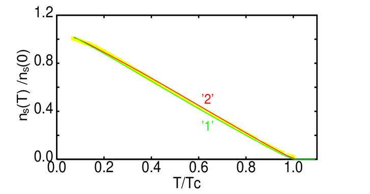
Figure 6: Calculated superfuid density, $n_{s}$, as a function of temperature, $T$, compared to the experimental data of Bonalde et al.[18] (gray squares). The line ’1’ shows the results for only $U^{\perp}_{m,m^{\prime}}(ij)<0$ while line ’2’ corresponds to the case where $U^{\perp}_{m,m^{\prime}}(ij)<0$ for $m,m^{\prime}=a,b$ and $U^{\parallel}_{c,c}(ij)<0$.

To describe superconductivity in Sr₂RuO₄, we start from the following simple multi-orbital attractive Hubbard Hamiltonian,

$$\hat{H} = \sum_{ijmm^{\prime},\sigma}\left((\varepsilon_{m}-\mu)\delta_{ij}\delta_{mm^{\prime}}-t_{mm^{\prime}}(ij)\right)\hat{c}^{+}_{im\sigma}\hat{c}_{jm^{\prime}\sigma}$$ (1)

$$-\frac{1}{2}\sum_{ijmm^{\prime}\sigma\sigma^{\prime}}U_{mm^{\prime}}^{\sigma\sigma^{\prime}}(ij)\hat{n}_{im\sigma}\hat{n}_{jm^{\prime}\sigma^{\prime}}.$$

Here $i$ and $j$ label the sites of a body centred tetragonal lattice (as shown in Fig. 1), and $m$ and $m^{\prime}$ refer to the three Ruthenium $t_{2g}$ orbitals (as shown in Fig. 2). In the following the orbitals will be denoted $a=xz$, $b=yz$ and $c=xy$. The hopping integrals $t_{mm^{\prime}}(ij)$ and site energies $\varepsilon_{m}$ were fitted to reproduce the experimentally determined three-dimensional Fermi surface [21, 22]. We found that the set $t_{mm^{\prime}}$ given in [12]gave a good account of the Fermi surface data.

Since the actual physical mechanism of pairing in Sr₂RuO₄ is unknown, we will adopt a phenomenological approach and treat the effective Hubbard interaction constants $U_{mm^{\prime}}^{\sigma\sigma^{\prime}}(ij)$ as free parameters. The idea is to test different “scenarios” for the interaction constants against the available experimental results. Good agreement between experiment and theory is likely to only occur when the interaction parameters $U_{mm^{\prime}}^{\sigma\sigma^{\prime}}(ij)$ lead to a gap function on the Fermi surface ${\bf d}({\bf k})$ which is similar to that actually present in the material. In particular, both the jump in specific heat at $T_{c}$, and the linear dependence of $C(T)/T$ ($C(T)/T\sim T$ for line nodes) near to $T=0$ are sensitive to the gap ${\bf d}({\bf k})$ over the whole Fermi surface. Scenarios in which the line nodes occur on all Fermi surface sheets or only on $\alpha$ $\beta$ would be expected to lead to different temperature dependencies of $C(T)$, which can therefore be distinguished by comparison to the experiments.

In Fig. 1 we depict schematically the possible interactions $U_{mm^{\prime}}^{\sigma\sigma^{\prime}}(ij)$ between electrons on the same Ru-atom (shown by circle ’1’) and the neighbouring Ru-atoms (shown by lines denoted ’2’,’3’ for in-plane and out of plane interactions, respectively). We assume that the dominant interaction between electrons on the same site $i$ (’1’) is the strong Coulomb repulsion. The effective interactions between nearest neighbours are assumed to be attractive. They could arise either from spin-fluctuation mediated exchange[4], or from interlayer Coulomb scattering[11].

In this paper we will compare two different model sets of interaction constants. The first is motivated by the inter-plane Coulomb scattering model of Koikegami, Yoshida and Yanagisawa[11]. It assumes Coulomb repulsion between electrons on the same and the nearest neighbour in plane lattice sites (’1’ and ’2’ in Fig. 1) and attraction between Ru planes (’3’ in Fig. 1). The corresponding Hubbard interaction parameters are

$${\bf U}^{\parallel}=\left(\begin{array}[]{ccc}0&0&0\\ 0&0&0\\ 0&0&0\end{array}\right)~{}~{}~{}~{}~{}~{}{\rm and}~{}~{}~{}~{}~{}~{}{\bf U}^{\perp}=\left(\begin{array}[]{ccc}U_{\perp}&U^{\perp}&0\\ U_{\perp}&U^{\perp}&0\\ 0&0&U^{\prime\perp}\end{array}\right),$$ (2)

expressed as matrices in orbital space, $m$, $m^{\prime}$. In this model there are two attractive Hubbard parameters, one acting only between $c$ orbitals and the other acting equally between $a$ and $b$ orbitals. In k-space there is little hybridization between the $a$-$b$ orbitals and the $c$ orbitals, and so these inter-plane interactions mainly corresponding to interactions within the $\gamma$ band ($U^{\prime\perp}$) and within the $\alpha$ and $\beta$ Fermi surface sheets ($U_{\perp}$). We shall call this case ’scenario 1’ in the rest of this paper.

We wish to compare the predictions of the above set of model parameters with those of our previous inter-plane coupling model[9, 10, 12], which was motivated by the different spatial orientations of the xz, yz, xy orbitals as shown in Fig. 2. Given that the Ru d-xy orbital ($c$) has a mainly 2-d character we assumed that interactions between $c$ orbitals are mainly in-plane. On the other hand the Ru d-xz (a) and d-yz (b) orbitals are oriented perpendicular to the RuO₂ plane, and so we assumed that the interactions between electrons in these orbitals are mainly iner-plane. This simple reasoning leads to the following two parameter Hubbard model with

$${\bf U}^{\parallel}=\left(\begin{array}[]{ccc}0&0&0\\ 0&0&0\\ 0&0&U^{\parallel}\end{array}\right)~{}~{}~{}~{}~{}~{}{\rm and}~{}~{}~{}~{}~{}~{}{\bf U}^{\perp}=\left(\begin{array}[]{ccc}U^{\perp}&U^{\perp}&0\\ U^{\perp}&U^{\perp}&0\\ 0&0&0\end{array}\right).$$ (3)

We shall refer to this as ’scenario 2’ below.

In our earlier papers[9, 10, 12] we showed that this simple model gives a good overall account of the temperature dependent heat capacity $C(T)$, in-plane superfluid density $n_{s}(T)$, and thermal conductivity. In [12] we showed that the predictions of the model are fairly robust against the addition of extra interaction parameters or disorder.

In equations 2 and 3 we have set to zero any interaction terms which are either assumed to be small, or those which may be repulsive. We have checked that all the zero values appearing in the above interaction matrices ${\bf U}^{\parallel}$ and ${\bf U}^{\perp}$ (Eqs. 2,3) can be changed into small positive values representing repulsions without any change to the solution, and so we decided to use (Eqs. 2,3) the minimal set leading to pairing.

For above choices of interactions within the negative $U$ extended Hubbard model (Eq. 1), we solved the Bogolubov-de Gennes equations:

$$\sum_{jm^{\prime}\sigma^{\prime}}\left(\begin{array}[]{ll}E^{\nu}-H_{m,m^{\prime}}(ij)&\Delta^{\sigma\sigma^{\prime}}_{m,m^{\prime}}(ij)\\ \Delta^{*\sigma\sigma^{\prime}}_{mm^{\prime}}(ij)&E^{\nu}+H_{mm^{\prime}}\end{array}\right)\left(\begin{array}[]{l}u^{\nu}_{jm\sigma^{\prime}}\\ v^{\nu}_{jm^{\prime}\sigma^{\prime}}\end{array}\right)=0$$ (4)

together with the self-consistency condition

$$\Delta^{\sigma\sigma^{\prime}}_{mm^{\prime}}=U^{\sigma\sigma^{\prime}}_{mm^{\prime}}(ij)\chi^{\sigma\sigma}_{mm^{\prime}}(ij);~{}~{}~{}~{}~{}\chi^{\sigma\sigma^{\prime}}_{mm^{\prime}}(ij)=\sum_{\nu}u^{\nu}_{im\sigma}v^{*\nu}_{jm^{\prime}\sigma^{\prime}}(1-2f(E^{\nu})),$$ (5)

which follow from Eq. (1) on making the usual BCS-like mean field approximation[23]. Here $f(E^{\nu})$ is the Fermi function, $\beta=1/k_{B}T$, $k_{B}$ is Boltzmann constant and $\nu$ enumerates the solutions of Eq. 4.

Assuming an p-wave pairing state of the form ${\bf d}({\bf k})\sim{\bf e}_{z}$, on each Fermi surface sheet, then we need only consider the gap parameters $\Delta^{\uparrow\downarrow}_{mm^{\prime}}(\bf k)$ at each point in the Brillouin zone. Dropping the spin indices for clarity, the general structure of pairing parameter is of the general form

$$\Delta_{mm^{\prime}}({\bf k})=\Delta^{x}_{mm^{\prime}}\sin{k_{x}}+\Delta^{y}_{mm^{\prime}}\sin{k_{y}}$$

$$+\Delta^{z}_{mm^{\prime}}\sin{k_{z}c\over 2}\cos{k_{x}\over 2}\cos{k_{y}\over 2}+\Delta^{f}_{mm^{\prime}}\sin{k_{x}\over 2}\sin{k_{y}\over 2}\sin{k_{z}c\over 2}$$

$$+\left(\Delta^{x}_{mm^{\prime}}\sin{k_{x}\over 2}\cos{k_{y}\over 2}+\Delta^{y}_{mm^{\prime}}\cos{k_{y}\over 2}\sin{k_{y}\over 2}\right)\cos{k_{z}c\over 2}$$ (6)

for $m,m^{\prime}=a$, $b$ and $c$. In the present calculations we neglected the possibilities of $p_{z}$ pairing ($\Delta^{z}_{mm^{\prime}}$) or f-wave pairing $\Delta^{f}_{mm^{\prime}}$, for reasons which are discussed further in [9, 12].

3 3. Line Nodes and Specific Heat

From the two different interaction models given by Eqs. 2 and 3 we numerically find the corresponding solutions of the gap equation Eqs. 4, 5. In the case of scenario ’1’, Eq. 2, the gap parameters have the general form,

$$\Delta_{mm^{\prime}}({\bf k})=\left(\Delta^{x}_{mm^{\prime}}\sin{k_{x}\over 2}\cos{k_{y}\over 2}+\Delta^{y}_{mm^{\prime}}\cos{k_{y}\over 2}\sin{k_{y}\over 2}\right)\cos{k_{z}c\over 2},$$ (7)

for $m,m^{\prime}=a,b,c$. While for scenario ’2’ (Eq. 3) the gap parameters are

$$\Delta_{cc}({\bf k})=\Delta^{x}_{cc}\sin k_{x}+\Delta^{y}_{cc}\sin k_{y}$$

$$\Delta_{mm^{\prime}}({\bf k})=\left(\Delta^{x}_{mm^{\prime}}\sin{k_{x}\over 2}\cos{k_{y}\over 2}+\Delta^{y}_{mm^{\prime}}\cos{k_{y}\over 2}\sin{k_{y}\over 2}\right)\cos{k_{z}c\over 2}$$ (8)

for $m,m^{\prime}=a$ or $b$, respectively. Clearly scenario ’1’ has a order parameter for which all of the gap parameters $\Delta_{mm^{\prime}}({\bf k})$ vanish in the planes $k_{z}=\pm\pi/c2$. Therefore all three Fermi surface sheets should have horizontal line nodes. On the other hand, in scenario ’2’ only the $a$ and $b$ components of $\Delta_{mm^{\prime}}({\bf k})$ vanish, implying that the $\gamma$ sheet is nodeless.

The temperature dependence of the order parameters in each scenario are shown in Fig. 3. In our analysis we have fitted the interaction parameters ($U^{\parallel}=-0.494t$, $U^{\perp}=-0.590t$, $U^{\prime\perp}=-0.312t$) to obtain a single critical temperature $T_{c}\approx 1.5$K for all order parameter components (Fig. 3). Note, the differences between $U^{\perp}=-0.590t$ and $U^{\prime\perp}=-0.312t$ arises as an effect of the difference in partial density of states for the bands $\alpha$, $\beta$ and $\gamma$. In case of $\gamma$ the Fermi surface is close to a Van Hove singularity [11, 24], and so $U^{\prime\perp}$ can be smaller while still obtaining the same $T_{c}$. On the other hand, the larger value of $U^{\perp}$ can be explained by the out of plane spatial orientation of the $a$ and $b$ Ru orbitals, compared to the in plane Ru d-xy orientation of $c$ orbital

The angular dependence of the eigenvalues $E_{k_{i},\rho}$, $i=x$, $y$ on the corresponding $\rho=\alpha$, $\beta$, $\gamma$ Fermi surface sheets, plotted along the $z$ axis, are shown in Fig. 4. In case of the inter-plane attraction only scenario ’1’ the gap has line nodes on all three Fermi surface sheets. In contrast, in scenario ’2’ the gap is nodeless on the $\gamma$ sheet, as can be seen in Fig 4(d).

Now the key question is whether experiment can distinguish between these two gap scenarios, namely line nodes on all Fermi surface sheets compared to just nodes on $\alpha$ $\beta$ only. We calculated the specific heat for those solutions via the following relation:

$$C=-2k_{B}\beta^{2}\frac{1}{N}\sum_{{\bf\rm k},\rho}E_{{\bf\rm k}\rho}\frac{\partial f(E_{{\bf\rm k}\rho})}{\partial\beta},$$ (9)

where $f$ is the Fermi function.

The results are presented in Fig. 5 and compared to the experimental values of Nishizaki et al.[17].

One can see in Fig. 5 that the slope of $C(T)/T$ near to $T=0$ is slightly higher for scenario ’1’ compared to scenario ’2’, consistent with the ”extra” line node on the $\gamma$ Fermi surface sheet. However the change in slope is quite small, and so one can say that either model is consistent with the low temperature experimental data.

On the other hand, in Fig. 5 it is clear that the second solution ’2’ works slightly better for the jump of specific heat at critical temperature $T_{c}$. Solution ’1’ has a smaller Fermi surface average of $|\Delta({\bf k})|^{2}$, and this leads to the slightly smaller jump in specific heat at $T_{c}$. The close similarity of curves ’1’ and ’2’ can be understood if one notices that the quite different gap symmetry on the $\gamma$ sheet can lead to rather similar results after integration over the Fermi surface (Eq. 10).

As a further test of the presence of horizontal line nodes on all Fermi surface sheets, we have also calculated the in-plane superfluid density $n_{s}(T)$ using

$$\frac{1}{\lambda^{2}(T)}=\mu_{0}e^{2}\sum_{\rho}\int_{BZ}{\rm d}^{3}k~{}v_{i}^{2}\left(\frac{\partial f}{\partial\epsilon_{{\bf\rm k}\rho}}-\frac{\partial f}{\partial E_{{\bf\rm k}\rho}}\right),$$ (10)

where $\lambda(T)$ denotes the temperature dependent penetration depth, $v_{i}=v_{x}$ or $v_{y}$ is the in plane band velocity at ${\bf\rm k}$, $e$ is the electron charge, $\mu_{0}=4\pi\times 10^{-7}$ is the magnetic constant, $\epsilon_{{\bf\rm k}\rho}$ is the electron band energy and

$$\frac{n_{s}(T)}{n_{s}(0)}=\frac{\lambda^{2}(0)}{\lambda^{2}(T)}.$$ (11)

Both secenarios ’1’ and ’2’ give similar results of $n_{s}$ and agree with experimental results by Bonalde et al.[18] (gray squares). However, one can note that the slightly different slope in small temperature regions gives a slight advantage to solution ’2’ which mimics the experimental data a little better.

4 4. Conclusions.

We have tested two different gap models for strontium ruthenate, which are consistent with two physically different pairing mechanisms. In scenario ’1’, we assumed that all in-plane interactions are repulsive, and that only the out of plane interactions lead to pairing. This is motivated by the Coulomb scattering pairing mechanism of Koikegami, Yoshida and Yanagisawa[11]. In scenario ’2’ we assumed attractive in-plane interactions for Ru $d-xy$ orbitals ($\gamma$ band) and attractive inter-plane interactions of the $a$ and $b$ orbitals ($\alpha$ and $\beta$ bands). Surprisingly we found that the predicted specific heat is very similar in both models (Fig. 5), even though one has a horizontal line node on all three Fermi surface sheets while the other has a nodeless $\gamma$ sheet. Similarly the temperature dependent superfuid density is closer to experiment in both scenarios. Of these two models the nodeless $\gamma$ sheet appears to be slightly close to the experiment, but the actual differences are small.

In these calculations we have not attempted to include the interband proximity effect proposed by Zhitomirsky and Rice[8]. In [12] we showed that this corresponds in real-space to the addition of three-site Hubbard interaction parameters, or assisted hopping, to the Hubbard Hamiltonian. It would be quite possible to combine this interband proximity effect interaction with either of the two pairing scenarios which we have considered here. However the close similarity of the specific heat and superfluid density in the two models, shown in Figs. 5, 6 strongly suggests that the effect of the proximity coupling terms would also be very similar in either pairing model.

References

- [1] Y. Maeno, H. Hashimoto, K. Yoshida, S. NishiZaki, T. Fujuta, J.G. Bednorz and F. Lichtenberg, Nature 372, 532 (1994).
- [2] Y. Maeno, T.M. Rice and M. Sigrist, Physics Today 54, 42 (2001).
- [3] A.P. Mackenzie, Y. Maeno, Rev. Mod. Phys. 75, 657 (2003).
- [4] D. Manske, I. Eremin, S.G. Ovchinnikov and J.F. Annett, unpublished.
- [5] Y. Hasegawa, K. Machida and M. Ozaki, J. Phys. Soc. Jpn. 69 336 (2000).
- [6] K. Kubo and D.S. Harashima, J. Phys. Soc. Jpn. 69 3489 (2000).
- [7] K. Kuboki, J. Phys. Soc. Jpn. 70, 2698 (2001).
- [8] M.E. Zhitomirsky and T.M. Rice, Phys. Rev. Lett. 87, 057001 (2001).
- [9] J.F. Annett, G. Litak, B.L. Györffy and K.I. Wysokiński, Phys. Rev. B 66, 134514 (2002)
- [10] K.I. Wysokinski, G. Litak, J.F. Annett and B.L. Györffy, Phys. Status Solidi B 236, 325 (2003).
- [11] S. Koikegami, Y. Yoshida and T. Yanagisawa, Phys. Rev. B 67 134517 (2003).
- [12] J. F. Annett, B.L. Györffy, G. Litak and K.I. Wysokiński, Eur. Phys. J. B in press, cond-mat/0306185.
- [13] Y. Hasegawa, M. Yakiyama, J. Phys. Soc. Jpn. 72, 1318 (2003).
- [14] K. Ishida, H. Mukuda, Y. Kitaoka, K Asayama, Z.Q. Mao, Y. Mori and Y. Maeno, Nature 396, 658 (1998).
- [15] J.A. Duffy, S.M. Hayden, Y. Maeno, Z. Mao, J. Kulda and G.J. McIntyre, Phys. Rev. Lett. 85, 5412 (2000).
- [16] G.M. Luke, Y. Fudamoto, K.M. Kojima, M.I. Larkin, J. Merrin, B. Nachumi, Y.J. Uemura, Y. Maeno, Z.Q. Mao, Y. Mori, H. Nakamura and M. Sigrist, Nature 394, 558 (1998).
- [17] S. NishiZaki, Y. Maeno and Z. Mao, J. Phys. Soc. Jpn 69, 336 (2000).
- [18] I. Bonalde, B.D. Yanoff, M.B. Salamon, D.J. van Harlingen, E.M.E. Chia, Z.Q. Mao and Y. Maeno, Phys. Rev. Lett. 85, 4775 (2000).
- [19] M. A. Tantar, M. Suzuki, S. Nagai, Z.Q. Mao Y. Maeno and T. Ishiguro, Phys. Rev. Lett. 86, 2649 (2001).
- [20] K. Izawa, H. Takahashi, H. Yamaguchi, Y. Matsuda, M. Suzuki, T. Sasaki, T. Fukase, Y. Yoshida, R. Settai and Y. Onuki, Phys. Rev. Lett. 86, 2653 (2001).
- [21] A.P. Mackenzie and Y. Maeno, Physica B 280, 148 (2000).
- [22] C. Bergemann, S.R. Julian, A.P. Mackenzie, S. NishiZaki and Y. Maeno, Phys. Rev. Lett. 84, 2662 (2000).
- [23] J.B. Ketterson and S.N. Song, Superconductivity, (Cambridge University Press, 1999).
- [24] G. Litak, J.F. Annett, and B.L. Györffy, Acta Phys. Pol. A 97, 249 (2000).
- [25] K. Miyake and D. Narikiyo, Phys. Rev. Lett. 83, 1423 (1999).