Global Phase Diagram of the High Tc Cuprates

Abstract

The high $T_{c}$ cuprates have a complex phase diagram with many competing phases. We propose a bosonic effective quantum Hamiltonian based on the projected $SO(5)$ model with extended interactions, which can be derived from the microscopic models of the cuprates. The global phase diagram of this model is obtained using mean-field theory and the Quantum Monte Carlo simulation, which is possible because of the absence of the minus sign problem. We show that this single quantum model can account for most salient features observed in the high $T_{c}$ cuprates, with different families of the cuprates attributed to different traces in the global phase diagram. Experimental consequences are discussed and new theoretical predictions are presented.

I Introduction

On the first look, the phase diagram of the high transition temperature superconducting (HTSC) cuprates has a striking simplicity: there are only three universal phases in the phase diagram of all HTSC cuprates: the antiferromagnetic (AF), the superconducting (SC) and the metallic phases, all with homogeneous charge distributions. However, closer inspection shows a bewildering complexity of other possible phases, which may or may not be universally present in all HTSC cuprates. A large class of these phases have inhomogeneous charge distributions. Because of this complexity, formulating an universal theory of HTSC is a great challenge. The $SO(5)$ theory unifies the AF and the SC order parameters into a single five dimensional order parameter called the superspin, and the effective quantum theory of the superspin naturally explains proximity between the AF and the SC phases in the observed phase diagramZhang (1997). The Goldstone modes of the superspin fluctuations can be identified with the $\pi$ resonance mode observed in the neutron scattering experimentsDemler and Zhang (1995, 1998); Rossatmignod et al. (1991); Mook et al. (1993); Fong et al. (1995); Dai et al. (1996); Fong et al. (1996); Mook et al. (1998); Dai et al. (1998); Fong et al. (2000, 1999); He et al. (2001, 2002); Stock et al. (unpublished); Tranquada et al. (unpublished). This theory also predicts the AF vortex stateZhang (1997); Arovas et al. (1997), which has recently been observed in a number of experimentsKatano et al. (2000); Mitrovic et al. (2001); Lake et al. (2001, 2002); Miller et al. (2002); Khaykovich et al. (2002); Mitrovic et al. (2003); Kang et al. (2003); Fujita et al. (unpublished). Initially, the $SO(5)$ theory was motivated by the simplicity of the pure AF and SC states, however, given the encouraging agreements with the experiments, it is tempting to construct an unified theory of the global phase diagram of the HTSC which addresses the more complex inhomogeneous phases as well. Complexities can of course be introduced phenomenologically into the Landau-Ginzburg type of theories by simply introducing more order parameters. However, this type of approach necessarily limits the predictive power of theory. The goal of this paper is to present a single effective quantum model of the superspin degree of freedom, which can be derived systematically from the microscopic electron models, and can be investigated reliably both analytically and numerically. The global phase diagram of this model is then compared with the experimentally observed phase diagram of the HTSC cuprates.

When formulated on a coarse-grained lattice, with high energy charge states projected out, the projected $SO(5)$ model describes five local superspin degrees of freedom per plaquetteZhang et al. (1999). These five states are the spin singlet state at half-filling, the spin triplet states at half-filling, and the singlet d-wave hole pair state. Using the Contractor Renormalization Group (CORE) algorithm, Altman and AuerbachAltman and Auerbach (2002) showed that the projected $SO(5)$ model can be systematically derived from the microscopic electron models, and they also determined the parameters of the effective $SO(5)$ model explicitly from the microscopic interaction parameters (see also Ref.[Capponi and Poilblanc, 2002]). Restricted within the subspace of these five local states, the Hamiltonian describing their propagation and interaction is completely expressed in terms of bosonic operators and can be studied reliably by the quantum Monte Carlo (QMC) calculations. The simplest form of the projected $SO(5)$ model has been studied extensively by the QMC method both in two dimensions Dorneich et al. (2002); Riera (2002a, b) and in three dimensions Jöstingmeier et al. (unpublished). The overall topology of the phase diagram, the scaling properties near the multi-critical point and the nature of the collective excitations can be reliably obtained from the QMC method, within the parameter regime of experimental interests.

The simplest form of the quantum $SO(5)$ model describe either the direct, first order transition from the AF to the SC state, or two second order transitions with an uniform, intermediate AF/SC mix phase in between the pure AF and the SC statesZhang (1997); Zhang et al. (1999). In the case of the direct first order transition as a function of the chemical potential, the system at a fixed density is phase separated. However, in the HTSC cuprates, there are other forms of charge and spin ordered states. For example, neutron scattering cross section in $LSCO$ material is peaked around $(\pi\pm\delta,\pi)$ and $(\pi,\pi\pm\delta)$, where $\delta\sim 1/8$Tranquada et al. (1995); Aeppli et al. (1997); Wells et al. (1997). STM experiments have revealed periodic charge modulation with period close to four lattice spacingHoffman et al. (2002); Howald et al. (2003), either near the vortex core or near surface impurities. In latter case, alternative interpretationMcElroy et al. (2003a); Wang and Lee (2003); McElroy et al. (2003b) based on quasi-particle interference is also possible, and the two points of views are summarized by Kivelson et al.Kivelson et al. (2003). Motivated by these experiments, we extend the simplest form of the projected $SO(5)$ model to include extended interactions among the five bosonic states. In fact, these extended interactions also arise naturally by carrying out the CORE algorithm to extended ranges.

The projected $SO(5)$ model with extended interactions support a more complex phase diagram. In particular, there are insulating phases at fractional filling factors where the charges form a lattice, usually commensurate with the underlying lattice. A crucial aspect of this model is that all charge density wave states are formed by the Cooper pairs of the holes, rather than the holes themselvesChen et al. (2002). Throughout this paper, we shall denote such states as the pair-density-wave (PDW) states or pair checkerboard states. This distinction has a profound experimental consequence, since the real space periodicity of the former is larger than the latter by a factor of $\sqrt{2}$. This type of insulating PDW states is a consequence of strong pairing and low superfluid density, a condition which is naturally fulfilled in the underdoped cuprates, but has not yet been unambiguously identified in other experimental systems before. The PDW state can either take the form of stripes or checkerboards, depending on the ratios of the extended interaction parameters in the model. Furthermore, PDW states with longer periodicity generally requires longer range interactions to stabilize. Based on this reasoning, a simple picture emerges for the global phase diagram of underdoped cuprates. The phase diagram consists of islands of insulating PDW states, each with a preferred rational filling fraction, immersed in the background of SC states (see Fig. 4). The height of the Mott insulating PDW lobes vary depending on the preferred filling fraction and the range of extended interactions, but in principle, these insulating states are all self-similar to each other, and similar to the parent AF insulator at half-filling. There can be either a direct first order phase transition, or two second order phase transitions between the SC state and the PDW state, with the possibility of an intermediate “supersolid” phase, where both orders are present.

Based on our model, the bewildering complexity of the cuprate phase diagram can be deduced from a simple principle of the “Law of Corresponding States”. This concept is borrowed from the work of Kivelson, Lee and Zhang on the global phase diagram of the quantum Hall effectKivelson et al. (1992), in fact, our proposed phase diagram in Fig. 4 bears great similarity to Fig. 1 of that reference. In the case of the QHE, the “Law of Corresponding States” physically relates all quantum phase transitions at various filling fractions to a single quantum phase transition from the $\nu=1$ integer state to the Hall insulator. In recent years, this powerful mapping among the different fractional states has been made more precise by the derivation of the $SL(2,Z)$ discrete modular group transformation from the Chern-Simons theoryPryadko and Zhang (1996); Burgess and Dolan (2001); Witten (unpublished). Similarly, the central idea of the current paper is to relate the fractional Mott insulator to SC transition with the transition from the AF Mott insulator at half-filling to SC state, which is already well understood within the context of the original, simple $SO(5)$ theory. The construction of the Mott insulating states at various fractional filling factors can be constructed from the “Law of Corresponding States”, iterated ad infinitum, to give a beautiful fractal structure of self-similar phases and phase transitions, as presented in Fig. 4. The various different compounds of the HTSC cuprates families have slightly different microscopic parameters, and they correspond to different slices of this global phase diagram. The global phase diagram provides a basic road-map to understand the common elements and differences among various HTSC compounds.

This paper mainly focuses on the zero temperature global phase diagram of the underdoped cuprates. However, it is understood that the model is valid below the pseudogap temperature, which we interpret as the temperature below which the system can be effectively described by the collective bosonic degrees of freedom, like the magnons and the hole pairs. Therefore, it is implied that the pseudogap state is a regime where the various ground states discussed here compete with each other, and different experiments may access different aspects of these competing states. The existence of the pseudogap temperature gives the fundamental experimental justification to investigate the global phase diagram of the underdoped cuprates by a purely bosonic model. In the future, we shall use the same model to investigate the manifestations of these competing states at finite temperature, in the pseudogap regime. A comparison of the charge order predicted by this work and the STM experiment in the pseudogap regime has recently been reported in Ref.[Chen et al., unpublished].

While this paper is presented within the logical context of the $SO(5)$ theory, some of the ideas and results bear intellectual similarities to the previous theoretical works. The idea of doped holes forming ordered stripes has been discussed extensively in Ref. [Zaanen and Gunnarsson, 1989; Tranquada et al., 1995; Tsunetsugu et al., 1995; Kivelson et al., 1998; White and Scalapino, 1998; Zaanen, 1999]. Although we focus more on the charged ordered states in the forms of checkerboards of hole pairs, they are conceptually related to stripes and can be realized experimentally or theoretically depending on the microscopic parameters. The pseudogap temperature was identified as the formation temperature of Cooper pairs by Emery and KivelsonEmery and Kivelson (1995). Our interpretation of the pseudogap temperature is more general, which also includes the formation of the magnetic collective modes in addition to the holes pairs. Vojta and SachdevVojta and Sachdev (1999) have discussed the phase diagram of doped Mott insulator with various charge ordered insulating states at rational fractions. More recently, Zhang, Demler and Sachdev have studied extensively the competition among charge and spin orderDemler et al. (2001); Zhang et al. (2002). Laughlin pointed out that the small superfluid density in the underdoped regime is responsible for various charge ordering phenomenaLaughlin (unpublished). Haas et al.Haas et al. (1995) have noticed that the Wigner crystal state of the hole pairs could be stabilized due to the competition of phase separation and long ranged Coulomb interaction. Kim and HorKim and Hor (2001) have discussed experiments at certain “magic” filling fractions in terms of the commensurate Wigner crystal type of order of the electrons, rather than the hole pairs discussed in this paper. Restricted to the charge sector, the projected $SO(5)$ model is essentially the same as the hard-core quantum boson model on a lattice, whose phase diagram has been extensively studiedFisher et al. (1989); Pich and Frey (1998); Hebert et al. (2002).

This paper is organized as follows. In section II, the projected $SO(5)$ model with extended interactions is presented. The choice of parameters is discussed from the CORE algorithm and phenomenology. The self-similarity of the insulating states and the classification of the quantum phase transitions are then discussed in section III. In section IV, the global phase diagram of the model is obtained within the mean field theory. The low energy collective modes and their quantum symmetry is then studied using a slave-boson approach. In section V, QMC simulation is carried out to compare with mean-field results obtained in section IV. The experimental consequences and predictions are discussed in section VI. Finally, section VII concludes our study.

II Hamiltonian of the model

The effective bosonic $SO(5)$ model can be derived directly from the microscopic Hubbard model or $t$-$J$ model, through a renormalization group transformation called the Contractor Renormalization(CORE) methodMorningstar and Weinstein (1996); Altman and Auerbach (2002). To construct bosonic quasiparticles from fermionic model, we divide the lattice into effective sites containing an even number of sites. In order to conserve the symmetry between $x$ and $y$-direction in the system, a plaquette of $2\!\times\!2$ sites are typically chosenZhang et al. (1999); Altman and Auerbach (2002). In their CORE study of the 2D Hubbard model, Altman and Auerbach Altman and Auerbach (2002) started from the spectrum of lowest-energy eigenstates of the 2$\times$2 plaquette for 0, 1 and 2 holes, respectively. The low energy eigenstates of the Heisenberg plaquette can be determined easily. The nondegenerate ground state $|\Omega\rangle$ (see Ref.[Altman and Auerbach, 2002] for a real-space representation in terms of the microscopic states on a plaquette) has energy $E_{0}\!=\!-2J$ and total spin $S\!=\!0$. This “RVB” like singlet state will be the vacuum state of the effective bosonic $SO(5)$ model. The next set of energy eigenstates are three triplet states $t^{\dagger}_{\alpha}|\Omega\rangle$ with energy $E_{t}\!=\!-J$ and total spin quantum number $S\!=\!1$. All other energy eigenstates of the Heisenberg plaquette have energies $E\!\geq\!0$ and can be neglected in the low energy effective model. It should be noted that the operator $t^{\dagger}_{\alpha}$ with spin $1$ and charge 0 create hardcore bosons because one cannot create more than one of them simultaneously on a single plaquette. The ground state of two holes is a “Cooper”-like hole pair with internal d-wave symmetry with respect to the vacuum.

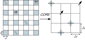
Figure 1: Illustration of the basic idea of the CORE method. To implement the CORE method, first decompose the original lattice in plaquettes, and then truncate the spectrum of a given plaquette to five lowest states, i.e, the singlet, hole-pair and three magnon states. An effective Hamiltonian for these bosons can then be determined using the CORE method. Left: local bosons in the original lattice. Gray rectangle denotes the singlet RVB vacua, circles denote holes and the set of two parallel vertical arrows denote the magnon. Right: local bosons on the lattice of plaquette. Leaf-like pattern denotes a local $d$-wave hole-pair on a plaquette. Canted arrow denotes local magnon on a plaquette. The singlet RVB vacuum is denoted by an empty site.

Using the CORE method and keeping only the five lowest states (the singlet boson, the three magnons $t^{\dagger}_{\alpha}$ and the hole-pair $t^{\dagger}_{h}$), the effective Hamiltonian of these bosons can be obtained asMorningstar and Weinstein (1996); Altman and Auerbach (2002); Capponi and Poilblanc (2002)

$${\cal H}={\cal H}_{0}+{\cal H}_{ext},$$ (1)

where ${\cal H}_{0}$ is the Hamiltonian of the previously studied $SO(5)$ model containing only on-site interactionsZhang et al. (1999); Jöstingmeier et al. (unpublished); Dorneich et al. (2002)

$${\cal H}_{0} = \Delta_{c}\sum_{i}t^{\dagger}_{h}(i)t_{h}(i)+\Delta_{s}\sum_{\alpha}\sum_{i}t^{\dagger}_{\alpha}(i)t_{\alpha}(i)$$ (2a)

$$- J_{c}\sum_{\langle ij\rangle}\left[t^{\dagger}_{h}(i)t_{h}(j)+H.c.\right]$$

$$- J_{s}\sum_{\alpha}\sum_{\langle ij\rangle}\left[t^{\dagger}_{\alpha}(i)+t_{\alpha}(i)\right]\left[t^{\dagger}_{\alpha}(j)+t_{\alpha}(j)\right],$$

and $${\cal H}_{ext}$$ is the part containing extended interactions

$${\cal H}_{ext} = \left[V_{c}\sum_{\langle ij\rangle}+V_{c}^{\prime}\sum_{\langle\langle ij\rangle\rangle}\right]n_{h}(i)n_{h}(j)$$ (2b)

$$- J_{\pi}\sum_{\alpha}\sum_{\langle ij\rangle}\left[t^{\dagger}_{h}(i)t_{h}(j)t^{\dagger}_{\alpha}(j)t_{\alpha}(i)+H.c.\right]$$

$$+ V_{\pi}\sum_{\alpha}\sum_{\langle ij\rangle}[n_{h}(i)n_{\alpha}(j)+n_{h}(j)n_{\alpha}(i)]$$

$$+ \sum_{\langle ij\rangle}\sum_{S=0,1,2}V_{S}\left(t_{i}t_{j}\right)^{\dagger}_{S}\left(t_{i}t_{j}\right)_{S}.$$

The model is subjected to the hard-core constraint

$$\sum_{\alpha}n_{\alpha}(i)+n_{h}(i)\leq 1.$$ (3)

Here, $\Delta_{c}$ and $\Delta_{s}$ are the energy costs to create a hole-pair and magnon respectively. $J_{c}$ and $J_{s}$ are the hopping terms of hole-pairs and magnons. $t_{h}(i)$ and $t^{\dagger}_{h}(i)$ are the annihilation and creation operators of hole-pair on plaquette $i$. $t_{\alpha}(i)$ and $t^{\dagger}_{\alpha}(i)$ are the annihilation and creation operators of magnon on plaquette $i$ for $\alpha=x,y,z$. $\langle\cdots\rangle$ and $\langle\langle\cdots\rangle\rangle$ denote nearest-neighbor(nn) and next-nearest-neighbor(nnn), respectively. $n_{h}(i)=t^{\dagger}_{h}(i)t_{h}(i)$ and $n_{\alpha}(i)=t^{\dagger}_{\alpha}(i)t_{\alpha}(i)$ are the hole-pair density and magnon density operators on plaquette $i$, respectively. The hole-pair density of $n_{h}$ per plaquette corresponds to twice the real doping of $\delta$ holes per lattice site, i.e.

$$\delta=n_{h}/2.$$ (4)

Finally, $\left(t_{i}t_{j}\right)^{\dagger}_{S}$ creates two magnons simultaneously on plaquettes $i$ and $j$, which are coupled into total spin $S$. ${\cal H}_{ext}$ contains nn and nnn hole pair interactions $V_{c}$ and $V_{c}^{\prime}$, exchange hopping terms $J_{\pi}$ between $t_{\alpha}$ and $t_{h}$ bosons, interaction $V_{\pi}$ between nn magnons and hole-pairs. The 4-magnon interactions $V_{0,1,2}$ are important in the pure AF phase but we can neglect them since we are mostly interested in the doped phase where magnon density decreases. According to the CORE calculation on 2-plaquettes and fixing $J_{s}=1$ as the unit of energy, one obtains from the $t$-J model with $J/t\simeq 0.4$ (relevant for cuprates) :

$J_{c}$	$J_{\pi}$	$V_{c}$	$V_{0}$	$V_{1}$	$V_{2}$	$V_{\pi}$
2.	-0.6	10	-1	-1	0.4	-3

For $J_{c}\sim 2$, ${\cal H}_{0}$ is approximately $SO(5)$ symmetric at the mean field levelZhang et al. (1999); Jöstingmeier et al. (unpublished); Dorneich et al. (2002).

The CORE derivation of the $SO(5)$ model (1) is only approximate. It should also be born in mind that the $t-J$ and the Hubbard models are also approximate models of the real cuprates themselves. If one started from a different microscopic model (for example, next-nearest neighbor hopping, extended Coulomb repulsion and etc), one would have obtained a similar effective Hamiltonian with different parameters. Therefore, in this paper, we shall take the CORE parameters as a guidance, and study the robust properties of the $SO(5)$ model with a more general set of parameters, as to reproduce well-known results and compare directly with experiments.

At half-filling ($n_{h}=0$), the model involves only the singlet and the magnon, and the effective Hamiltonian containing only $J_{s}$ and $\Delta_{s}$ can be rewritten as

$$H=2J_{s}\sum_{\langle ij\rangle}\frac{t^{\dagger}_{\alpha}(i)+t_{\alpha}(i)}{\sqrt{2}}\frac{t^{\dagger}_{\alpha}(j)+t_{\alpha}(j)}{\sqrt{2}}+\frac{\Delta_{s}}{2}\sum_{i}L_{\alpha\beta}^{2}(i),$$ (5)

where $[t^{\dagger}_{\alpha}(i)+t_{\alpha}(i)]/\sqrt{2}$ is the AF moment and $L_{\alpha\beta}(i)$ is the $SO(3)$ symmetry generatorZhang et al. (1999)

$$L_{\alpha\beta}(i)=-i[t^{\dagger}_{\alpha}(i)t_{\beta}(i)-t^{\dagger}_{\beta}(i)t_{\alpha}(i)].$$ (6)

This model is similar to the nonlinear $\sigma$ model (NL$\sigma$M)Chakravarty et al. (1988); Manousakis (1991)

$$H=\rho_{s}\sum_{\langle ij\rangle}m_{i}^{\alpha}m_{j}^{\alpha}+\frac{1}{\chi}\sum_{i}S^{2}_{i},$$ (7)

where $m_{i}^{\alpha}$ is the $\alpha$ component of the AF moment and $S_{i}$ is the angular moment on site $i$. After rescaling of time using the spin velocity $c=\sqrt{\rho_{s}/\chi}$ and up to a prefactor, the Lagrangian density of the NL$\sigma$M can be cast in the usual form in the continuum limit

$$\mathcal{L}_{NL\sigma}=\frac{1}{g}(\partial_{x}m)^{2}+g(\partial_{\tau}m)^{2},$$ (8)

where $g\sim 1/\sqrt{\rho_{s}\chi}$ is a dimensionless constant. This model has been studied extensively Manousakis (1991). It has a transition towards a disordered state at $g_{c}=1.45$. From the computation of the staggered moment, we can find $g$ such that the original Heisenberg value (0.3) of the AF moment is recovered: $g_{H}=1.125$. On the other hand, we know from mean-field calculations and QMC simulation that the disordered phase occurs at $\Delta_{s}/J_{s}=8$. We then obtain the proportionality factor between $g$ and $1/\sqrt{\rho_{s}\chi}$. Using $g_{H}$, we find that an effective model for Heisenberg corresponds to $\Delta_{s}/J_{s}=4.8$.

In most parts of this paper, we shall consider the simplified model with $J_{\pi}=V_{\pi}=0$.

III Heuristic argument on the self-similarity between pair-density-wave (PDW) states

Let us ignore for a moment the magnons, and consider a hard-core boson model with extended interactions. The phase diagramFisher et al. (1989); Pich and Frey (1998) of a hard-core boson model with nn interaction contains one superfluid state and three Mott-insulating states, corresponding to zero-doping ($n_{h}=0$), half-filling ($n_{h}=1/2$) and fully-occupied ($n_{h}=1$), as sketched in Fig. 2. The half-filling state has checkerboard charge order. If one transforms the hard-core boson model into an AF Heisenberg model, the checkerboard order of the bosons simply correspond to the AF order of the Heisenberg spins. The following argument assumes that the checkerboard order at half-filling is a basic and robust form of order, such that it is repeated at all different levels of the hierarchy.

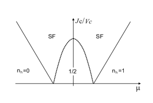
Figure 2: Phase diagram of a hard-core boson model with nearest-neighbor interaction. There are one superfluid (SF) state and three insulating states: zero-doping state ($n_{h}=0$), half-filled state ($n_{h}=1/2$) and fully-occupied state ($n_{h}=1$). At the next level of the hierarchy, longer ranged interactions lead to new insulating states with $n_{h}=1/4$ and $n_{h}=3/4$, as shown in Fig. 3.

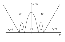
Figure 3: Phase diagram of a hard-core boson model with nn and nnn interactions. There are a superfluid (SF) state and five insulating states with doping $0/4,1/4,2/4,3/4$ and $4/4$. At the next level of the hierarchy, new insulating states are developed at doping level $n_{h}=1/8$, $n_{h}=3/8$, $n_{h}=5/8$ and $n_{h}=7/8$. This hierarchy construction can be iterated ad infinitum, to obtain a self-similar phase diagram with insulating phases at doping level $p/2^{n}$, with integers $p$ and $n$, such that $0<p<2^{n}$.

If we regard the empty sites of the half-filled checkerboard state as an inert background, we obtain a fully-occupied Mott-insulating state on the coarse-grained lattice, with lattice spacing $\sqrt{2}a\times\sqrt{2}a$. The nnn interaction on the original lattice becomes the nn interaction on the coarse-grained lattice, and a new half-filled checkerboard state can be stabilized on the coarse-grained lattice. Such a state corresponds to doping $n_{h}=1/4$ on the original lattice. Similarly, we can regard the filled sites of the original half-filled checkerboard lattice as an inert background, leaving with an empty state on the coarse-grained lattice. A new checkerboard state can again be stabilized on the coarse-grained lattice, which corresponds to doping $n_{h}=3/4$ on the original lattice. This hierarchical procedure of forming a new daughter checkerboard state from two parent checkerboard state can obviously be iterated ad infinitum, to obtain a fractal-like, self-similar phase diagram as shown in Fig.3. It is interesting to note that the nearest-neighbor interaction on the coarse-grained lattice is just the next-nearest-neighbor interaction on the original lattice. There is also the possibility that small regions with coexisting SF and PDW orders (“supersolids”) are present around the Mott-insulating lobes in the phase diagram Pich and Frey (1998); Vanotterlo and Wagenblast (1994); Batrouni et al. (1995); Hebert et al. (2002).

Having presented the generic phase diagram for the charge boson only, we consider now the inclusion of the magnons in the full $SO(5)$ with extended interactions. Generally, charge ordered insulating states also have AF order. The $n_{h}=0$ state of the charge boson corresponds to the undoped parent Mott insulator. The $n_{h}=1/2$ state of the charge boson would correspond to $\delta=1/4$ doping for the cuprates, which is probably at or beyond the limit of applicability of our bosonic model. Therefore, the phase diagram of the hard-core boson model in the range of $0<n_{h}<1/2$ from Fig. 3 would translate into a phase diagram of the cuprates in the doping range of $0<\delta<1/4$, as shown in Fig. 4. As we shall show later, this phase diagram is supported by accurate QMC calculations of the $SO(5)$ model with extended interactions. We expect that the insulating states of $\delta=1/16$ and $1/8$ are AF ordered. Since the magnon density decreases with increasing doping, the $\delta=3/16$ state may not be AF ordered.

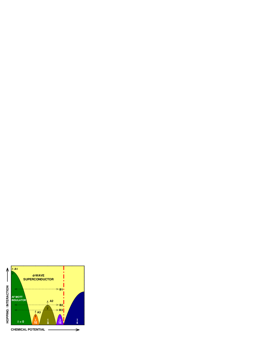
Figure 4: A typical global phase diagram of the cuprates in the parameter space of chemical potential and the ratio of boson hopping energy over Coulomb interaction energy. This phase diagram shows self-similarity among the insulating PDW states at half-filling and other rational filling fractions. There are two types of superfluid-insulator transition. The quantum phase transition of “class A” can be approached by varying the hopping energy, for example, by applying a pressure and magnetic field at constant doping. The quantum phase transition of “class B” can be realized by changing the chemical potential or doping. There can be either a direct first order phase transition, or two second order phase transitions between the SC state and the PDW state, with the possibility of an intermediate “supersolid” phase, where both orders are present. Different families of cuprates correspond to different traces of “class B”. For example, we believe $YBCO$ is $B1$-like, $BSCO$ may be close to $B2$-like and $LSCO$ is $B3$-like. The vertical dash-dot line denotes a boundary in the overdoped region beyond which our pure bosonic model becomes less accurate.

The nature of the phase boundary between two different phases shown in Fig. 4 requires careful characterization. We can classify all phase transitions into two broad classes. Class $A$ describes transitions at fixed chemical potential, typically at an effectively particle-hole symmetric point around the tip of the Mott lobe. Class $B$ describes transitions where the chemical potential or the density is varied. Each broad class is further classified into three types, $1$, $2$ and $1.5$. Generically, the phase transition between two ordered phase can be either a single first-order transition or two second order transitions, with a mixed state in between, where both order parameters are nonzero. A third marginal possibility occurs at a symmetric point, when these two second order phase transitions collapse into a single one. In the context of high Tc cuprates, these three types are shown in phase diagrams of Ref.[Zhang, 1997] as Fig. 1a,b,c, respectively. This situation can be easily understood by describing the competition in terms of a Landau-Ginzburg functional of two competing order parametersKosterlitz et al. (1976), which is given by

$$F=\frac{1}{2}r_{1}\phi_{1}^{2}+\frac{1}{2}r_{2}\phi_{2}^{2}+u_{1}\phi_{1}^{4}+u_{2}\phi_{2}^{4}+2u_{12}\phi_{1}^{2}\phi_{2}^{2}$$ (9)

where $\phi_{1}$ and $\phi_{2}$ are vector order parameters with $N_{1}$ and $N_{2}$ components, respectively. In the context of $SO(5)$ theory, $N_{1}=2$ and $N_{2}=3$, and we can view $\phi_{1}^{2}$ as SC component of the superspin vector, and $\phi_{2}^{2}$ as the AF component of the superspin vector. These order parameters are obtained by minimizing the free energy $F$. By tuning $r_{1}$, one can drive a quantum phase transition from AF to SC. For $u_{12}>\sqrt{u_{1}u_{2}}$, the quantum phase transition from AF to SC is a single first order transition of “type $1$”. For $u_{12}<\sqrt{u_{1}u_{2}}$, the transition from AF to SC consists in two second order transitions, and there is a finite range of $r_{1}$ where AF and SC coexist uniformly; the transition is of “type $2$”. For $u_{12}=\sqrt{u_{1}u_{2}}$, the phase transition occurs at

$$\frac{r_{1}}{\sqrt{u_{1}}}=\frac{r_{2}}{\sqrt{u_{2}}},$$ (10)

where the free energy takes the $SO(5)$ symmetric form

$$F=\frac{r_{1}\sqrt{u_{1}}}{2}\tilde{\phi}^{2}+u_{12}^{2}\tilde{\phi}^{4}$$ (11)

with

$$\tilde{\phi}^{2}=\frac{\phi_{1}^{2}}{\sqrt{u_{1}}}+\frac{\phi_{2}^{2}}{\sqrt{u_{2}}}.$$ (12)

Since the free energy depends only on $\tilde{\phi}$, one order parameter can be smoothly rotated into the other without any energy cost. At this point, the chemical potential is held fixed, but the SC order parameter and the charge density can change continuously according the condition that $\tilde{\phi}^{2}$ is constant. This is a special case intermediate between “type $1$ and $2$” transitions, where two second order phase transitions collapse into one. This transition can only occur at a $SO(5)$ symmetric point. We thus classify it as “type $1.5$”. The full quantum $SO(5)$ symmetry can only be realized in the class $A$ transition of “type $1.5$”. On the other hand, the static, or projected $SO(5)$ symmetry can be realized in class $B$ transitions of “type $1.5$”.

In HTSC cuprates, the charge gap at half-filling is very large, of the order of $U\sim 6eV$ , it is not possible to induce the “class A1” transition from the AF to the SC state by conventional means. However, the charge gap in the fractional insulating states is much smaller, of the order of $J_{c}$, and it is possible to induce the “class A2” or “class A3” insulator to superconductor transition by applying pressureArumugam et al. (2002); Sato et al. (2000) or by applying a magnetic fieldHawthorn et al. (2003); Sun et al. (2003).

As the chemical potential or the doping level is varied, a given system, roughly corresponding to a fixed value of the quantum parameter $J_{c}/V_{c}$ , traces out different one dimensional slices in this phase diagram, with typical slices $B1$, $B2$ and $B3$ depicted in Fig. 4. The nature of the phase transition $B1$ is similar to that of the superspin-flop transition discussed in Ref.[Zhang, 1997]. In this case, the phase transition from the AF to the SC state can be further classified into “types 1, 1.5 and 2”, with the last two cases leading to a AF/SC mixed phase at the phase transition boundary. For lower values of $J_{c}/V_{c}$ , the trace $B3$ encounters the $\delta=1/8$ insulating phase. The key signature of this type of phase transition is that the SC $T_{c}$ will display a pronounced minimum as the doping variation traces through the $\delta=1/8$ insulating state. Meanwhile, the AF ordering (possibly at a wave vector shifted from $(\pi,\pi)$) will show reentrant behavior as doping is varied. The phase transition around the fractional insulating phases can again be classified into types “1, 1.5 and 2”, with possible AF/SC, AF/PDW, SC/PDW and AF/PDW/SC mixed phases.

We believe that the AF to SC transition in the $YBCO$, $BCCO$ and the $NCCO$ systems corresponds to a “class B1” transition. These systems only have a AF to SC transition, which can be further classified into types “1, 1.5 and 2”, but they do not encounter additional statically ordered fractional insulating phases. On the other hand, the phase transition in the $LSCO$ system, where $T_{c}$ displays a pronounced dip at $\delta=1/8$, correspond to the “class B3” transition.

IV Mean-field phase diagram of the model

IV.1 Four-sublattice ansatz and mean-field phase diagram

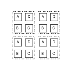
Figure 5: The schematic plot of the unit cell of a quarter-filled magnetic insulating state. The solid square denotes a plaquette of the original lattice and the dash-dot square denotes a $2$-plaquette by $2$-plaquette unit cell.

Since the Hamiltonian (1) contains up to nnn interactions, we can introduce the following four-sublattice ansatz within mean field theory:

$$|\Psi\rangle=\prod_{r,m}\left[e_{m}+h_{m}t_{h}^{\dagger}(m,r)+x_{m}t_{x}^{\dagger}(m,r)\right]|\Omega\rangle$$ (13)

where $|\Omega\rangle$ is the singlet ground state, $e_{m},x_{m},h_{m}$ are real variational parameters, $m=A,B,C,D$ denote the sites in a unit cell, and $r$ is the coordinate in the lattice of unit cells, as sketched in Fig. 5. The mean-field energy $E_{MF}$ reads

$$\frac{4E_{MF}}{N}=\Delta_{c}\left(h_{A}^{2}+h_{B}^{2}+h_{C}^{2}+h_{B}^{2}\right)-2J_{c}\left[e_{A}h_{A}+e_{C}h_{C}\right]\left[e_{B}h_{B}+e_{D}h_{D}\right]+\Delta_{s}\left(x_{A}^{2}+x_{B}^{2}+x_{C}^{2}+x_{B}^{2}\right)$$

$$-4J_{s}\left[e_{A}x_{A}+e_{C}x_{C}\right]\left[e_{B}x_{B}+e_{D}x_{D}\right]-4J_{\pi}\left[h_{A}x_{A}+h_{C}x_{C}\right]\left[h_{B}x_{B}+h_{D}x_{D}\right]+2V_{c}[h_{A}^{2}+h_{C}^{2}][h_{B}^{2}+h_{D}^{2}]$$

$$+4V_{c}^{\prime}[h_{A}^{2}h_{C}^{2}+h_{B}^{2}h_{D}^{2}]+2V_{\pi}\left([h_{A}^{2}+h_{C}^{2}][x_{B}^{2}+x_{D}^{2}]+[h_{B}^{2}+h_{D}^{2}][x_{A}^{2}+x_{C}^{2}]\right)$$ (14)

with the hard-core constraint

$$h_{m}^{2}+x_{m}^{2}+e_{m}^{2}=1,\quad m=A,B,C,D.$$ (15)

Here, $N/4$ is the number of unit-cells and $N$ is the number of plaquettes.

By minimizing the energy functional (14) subjected to the hard-core constraint (15), we obtain the mean-field ground state for a given set of parameters. Fig. 6 plots the mean-field global phase diagram, for $\Delta_{s}=4.8$, $V_{c}=4.1010$, $V_{c}^{\prime}=3.6329$ and $J_{\pi}=V_{\pi}=0$.

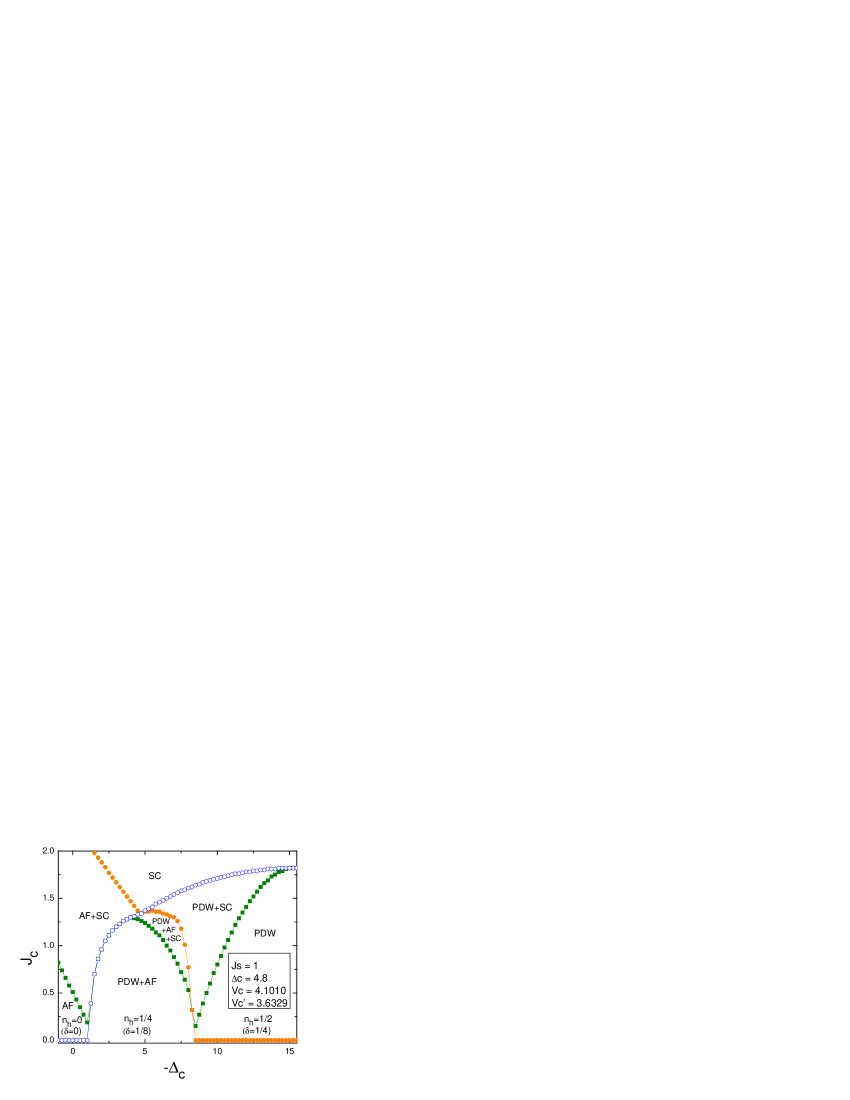
Figure 6: The MF phase diagram obtained by minimizing the energy functional (14) subjected to the hard-core constraint (15). $J_{\pi}$ and $V_{\pi}$ are taken to be zero.

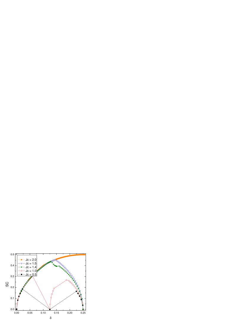
Figure 7: Doping dependence of SC order parameter for different $J_{c}$. For small $J_{c}$, there is a dip around hole-pair doping $n_{h}=1/4$ (real doping $\delta=1/8$).

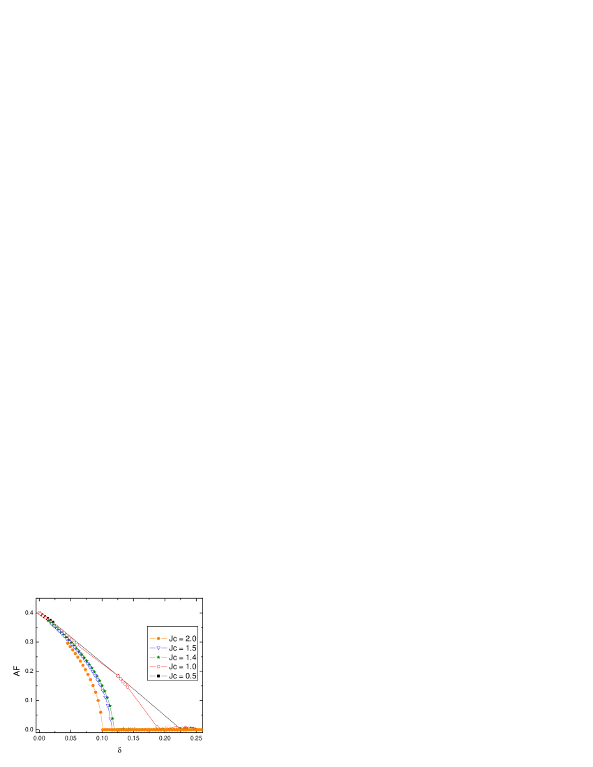
Figure 8: Doping dependence of AF order parameter for different $J_{c}$. For $J_{c}>1.3$, AF order decreases as doping increases and vanishes around $\delta=0.1$.

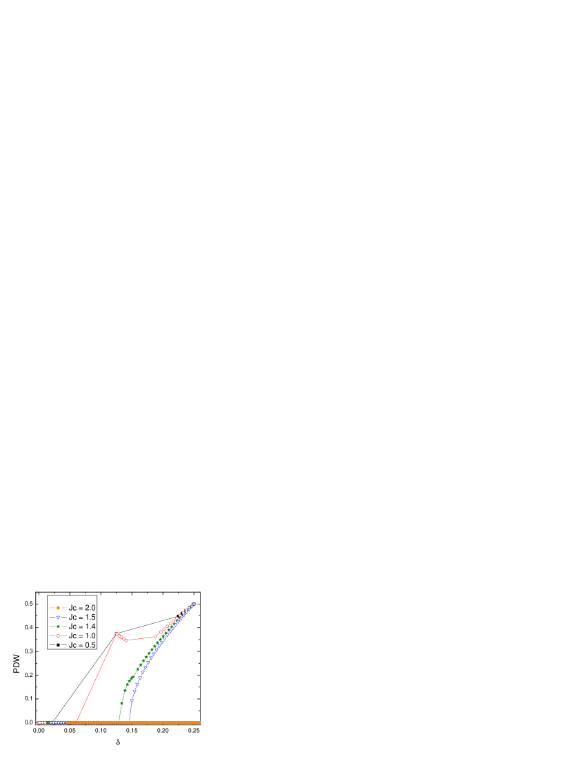
Figure 9: Doping dependence of PDW order defined for difference $J_{c}$. For $J_{c}<1.3$, a strong peak is present at $n_{h}=1/4$ or real doping $\delta=1/8$.

This phase diagram displays some rich features as expected. It has three insulating state: an undoped antiferromagnetic (AF) state, an insulating AF PDW state with hole-pair density $n_{h}=1/4$ ($\delta=1/8$) and an insulating PDW state with hole-pair density $n_{h}=1/2$ ($\delta=1/4$). Besides these insulating states, it also has a pure SC phase, a supersolid phase and mix phases of coexisting AF and SC order.

In Fig. 7 and Fig. 8, we plot the doping dependence of SC and AF orders for different $J_{c}$. If one follows a “class B1” trace, such as the one with fixed $J_{c}=1.5$, the doping dependence of SC order mimics the behavior of $YBCO$ and $BSCO$ families with a underdoped region $n_{h}<0.3(\delta<0.15)$ and an overdoped region $n_{h}>0.3(\delta>0.15)$. If one follows a “class B3” trace, such as the one with fixed $J_{c}=1.0$, the SC order displays a pronounce dip and the AF ordering is strongly enhanced around $n_{h}=1/4$ ($\delta=1/8$). Therefore, the “class B2” trace mimics the behavior of $LSCO$ family.

The doping dependence of charge order parameter is also plotted in Fig. 9. It measures the charge modulation defined by

$$PDW=\frac{1}{4}\sum_{m}\left|n_{h}(m)-n_{h}\right|$$ (16)

where $n_{h}$ is the average hole-pair density and $m$ is summed over $A,B,C,D$. While “class B1” trace shows no charge ordering in underdoped region, “class B3” trace displays a clear signature of charge ordering around $\delta=1/8$.

IV.2 Slave-boson approach, effective Hamiltonian and dynamical $SO(5)$ symmetry

The hard-core constraint (3) can also be enforced by introducing a slave-boson $t_{e}^{\dagger}(i)$ for each latticeZhang et al. (1999). The presence of this boson indicates that the plaquette $i$ is empty. The hard-core condition (3) is then replaced by

$$\hat{Q}(i)=\left(\sum_{\alpha}t^{\dagger}_{\alpha}t_{\alpha}(i)+t^{\dagger}_{h}t_{h}(i)+t_{e}^{\dagger}t_{e}(i)-1\right)=0.$$ (17)

This constraint can be enforced by introducing an additional site dependent field $\lambda(i)$ and adding to the Hamiltonian (1) an additional term

$$H_{\lambda}=-\sum_{i}\lambda(i)Q(i).$$ (18)

Since in physical states one always has one and only one boson per lattice sites, destruction (creation) of a boson $t_{a}(t_{a}^{\dagger})$, $a=x,y,z,h$, must always be accompanied by creation (destruction) of the empty boson $t_{e}^{\dagger}(t_{e})$. In this way, the whole Hamiltonian takes the form

$${\cal H}_{sb} = \Delta_{c}\sum_{i}t^{\dagger}_{h}(i)t_{h}(i)+\Delta_{s}\sum_{i}t^{\dagger}_{\alpha}(i)t_{\alpha}(i)$$ (19)

$$-J_{c}\sum_{\langle ij\rangle}\left[t^{\dagger}_{h}(i)t_{e}(i)t_{e}^{\dagger}(j)t_{h}(j)+H.c.\right]$$

$$-J_{s}\sum_{\langle ij\rangle}\left[t^{\dagger}_{\alpha}t_{e}(i)+t_{e}^{\dagger}t_{\alpha}(i)\right]\left[t^{\dagger}_{\alpha}t_{e}(j)+t_{e}^{\dagger}t_{\alpha}(j)\right]$$

$$-\sum_{i}\lambda(i)Q(i)+{\cal H}_{ext}$$

By integrating out the $\lambda$ field in the partition function, one automatically enforces the hard-core constraint $Q(i)=0$ on each site. The saddle point approximation to (19) corresponds to replacing the boson operators and $\lambda$ field with real constants to minimize the energy. Within the four-sublattice ansatz, this is equivalent to minimizing the energy functional subjected to the hard-core constraint (15). After obtaining the ground state, we can expand the boson operators around their mean-field values and drop quartic terms in the Hamiltonian (19) to yield an effective Hamiltonian of the boson operators around the ground state.

We shall now study the checkerboard state characterized by following mean-field solution:

$$h_{A}=1,x_{A}=e_{A}=h_{B}=h_{C}=h_{D}=0$$ (20)

for the simplified model with $J_{\pi}=V_{\pi}=0$.

The saddle-point of the slave-boson Hamiltonian (19) can be solved to yield

$$x_{D} = x_{B}=x_{C}=0$$ (21a)

$$e_{D} = e_{B}=e_{C}=1$$ (21b)

$$\lambda_{D} = =\lambda_{B}=\lambda_{C}=0$$ (21c)

$$\lambda_{A} = \Delta_{c}$$ (21d)

for $\Delta_{s}/Js\geq 4\sqrt{2}$ and

$$x_{D} = x_{B}=\sqrt{\frac{1}{16}\left[8-\frac{\Delta_{s}}{J_{s}}\sqrt{\frac{64J_{s}^{2}+\Delta_{s}^{2}}{16J_{s}^{2}+\Delta_{s}^{2}}}~{}\right]}\quad\quad e_{D}=e_{B}=\sqrt{\frac{1}{16}\left[8+\frac{\Delta_{s}}{J_{s}}\sqrt{\frac{64J_{s}^{2}+\Delta_{s}^{2}}{16J_{s}^{2}+\Delta_{s}^{2}}}~{}\right]}$$ (22a)

$$x_{C} = \sqrt{\frac{1}{8}\left[4-\frac{\Delta_{s}}{J_{s}}\sqrt{\frac{16J_{s}^{2}+\Delta_{s}^{2}}{64J_{s}^{2}+\Delta_{s}^{2}}}~{}\right]}\quad\quad\quad\quad\quad e_{C}=\sqrt{\frac{1}{8}\left[4+\frac{\Delta_{s}}{J_{s}}\sqrt{\frac{16J_{s}^{2}+\Delta_{s}^{2}}{64J_{s}^{2}+\Delta_{s}^{2}}}~{}\right]}$$ (22b)

$$\lambda_{C} = \frac{\Delta_{s}}{2}-2J_{s}\sqrt{\frac{64J_{s}^{2}+\Delta_{s}^{2}}{16J_{s}^{2}+\Delta_{s}^{2}}}\quad\quad\quad\quad\quad\quad\quad\quad\lambda_{A}=\Delta_{c}$$ (22c)

$$\lambda_{D} = \lambda_{B}=\frac{\Delta_{s}}{2}-4J_{s}\sqrt{\frac{16J_{s}^{2}+\Delta_{s}^{2}}{64J_{s}^{2}+\Delta_{s}^{2}}}$$ (22d)

for $\Delta_{s}/J_{s}\leq 4\sqrt{2}$.

The bosons are then expanded around their mean-field values as

$$t_{h}(m,r)=h_{m}+\hat{b}_{h}(m,r),$$ (23a)

$$t_{x}(m,r)=x_{m}+\hat{b}_{x}(m,r),$$ (23b)

$$t_{e}(m,r)=e_{m}+\hat{b}_{e}(m,r),$$ (23c)

$$t_{y}(m,r)=\hat{b}_{y}(m,r),$$ (23d)

$$t_{z}(m,r)=\hat{b}_{z}(m,r).$$ (23e)

Again, $m=A,B,C,D$ and $r$ is the coordinate in the coarse-grained lattice of unit cells. Plug (23a)-(23e) into the slave-boson Hamiltonian (19) and drop the quartic terms to yield the quadratic effective Hamiltonian

$$H^{eff}=E_{0}+H_{h}^{eff}+H_{x}^{eff}+H_{y}^{eff}+H_{z}^{eff}$$ (24)

with $E_{0}$ the mean-field ground state energy given by

$$E_{0} = 2N(\Delta_{c}-\lambda_{B})x_{B}^{2}+N(\Delta_{c}-\lambda_{C})x_{C}^{2}$$ (25a)

$$+4Nx_{C}e_{C}x_{B}e_{B}$$

and $$H^{eff}_{x} H^{eff}_{h} H^{eff}_{y} H^{eff}_{z}$$,, and

$$H^{eff}_{x} = \sum_{m=B,C,D}\left[\sum_{q}(\Delta_{s}-\lambda_{m})\hat{b}^{\dagger}_{x}\hat{b}_{x}(m,q)-\sum_{q}\lambda_{m}\hat{b}^{\dagger}_{e}\hat{b}_{e}(m,q)\right]$$ (25b)

$$-J_{s}\sum_{q}\bigg{[}4e_{B}x_{B}\biggl{(}\hat{b}^{\dagger}_{x}(C,q)\hat{b}_{e}(C,q)+H.c.\biggr{)}+B\leftrightarrow C\bigg{]}$$

$$-2J_{s}\sum_{q}\bigg{[}e_{C}[\hat{b}^{\dagger}_{x}(C,q)+\hat{b}_{x}(C,-q)]+x_{C}[\hat{b}^{\dagger}_{e}(C,q)+\hat{b}_{e}(C,-q)]\bigg{]}\times$$

$$\quad\bigg{[}\cos q_{x}\biggl{(}e_{B}[\hat{b}^{\dagger}_{x}(B,-q)+\hat{b}_{x}(B,q)]+x_{B}[\hat{b}^{\dagger}_{e}(B,-q)+\hat{b}_{e}(B,q)]\biggr{)}+\cos q_{y}\biggl{(}B\leftrightarrow D\biggr{)}\bigg{]}$$

$$H_{h}^{eff} = \sum_{q}\left(\Delta_{c}-\lambda_{B}+2V_{c}\right)\left[\hat{b}^{\dagger}_{h}\hat{b}_{h}(B,q)+\hat{b}^{\dagger}_{h}\hat{b}_{h}(D,q)\right]+\sum_{q}\left(\Delta_{c}-\lambda_{C}+4V_{c}^{\prime}\right)\hat{b}^{\dagger}_{h}\hat{b}_{h}(C,q)$$ (25c)

$$+ \sum_{q}(\Delta_{s}-\Delta_{c})\hat{b}_{x}^{\dagger}\hat{b}_{x}(A,q)-\lambda_{A}\sum_{q}\hat{b}^{\dagger}_{e}\hat{b}_{e}(A,q)-J_{s}\sum_{q}8e_{B}x_{B}~{}[\hat{b}^{\dagger}_{x}(A,q)\hat{b}_{e}(A,q)+\hat{b}^{\dagger}_{e}(A,q)\hat{b}_{x}(A,q)]$$

$$- 2J_{c}e_{B}\sum_{q}\biggl{[}\cos q_{y}\biggl{(}\hat{b}_{e}(A,q)\hat{b}_{h}(B,-q)+\hat{b}^{\dagger}_{h}(B,-q)\hat{b}^{\dagger}_{e}(A,q)\biggr{)}+\cos q_{x}\biggl{(}B\leftrightarrow D\biggr{)}\biggr{]}$$

$$- 2J_{c}e_{B}e_{C}\sum_{q}\biggl{[}\cos q_{x}\biggl{(}\hat{b}^{\dagger}_{h}(C,q)\hat{b}_{h}(B,q)+\hat{b}^{\dagger}_{h}(B,q)\hat{b}_{h}(C,q)\biggr{)}+\cos q_{y}\biggl{(}B\leftrightarrow D\biggr{)}\biggr{]}$$

$$H_{\alpha}^{eff}=\sum_{q}(\Delta_{s}-\lambda_{B})\left(\hat{b}_{\alpha}^{\dagger}\hat{b}_{\alpha}(B,q)+\hat{b}_{\alpha}^{\dagger}\hat{b}_{\alpha}(D,q)\right)+\sum_{q}(\Delta_{s}-\lambda_{C})\hat{b}_{\alpha}^{\dagger}\hat{b}_{\alpha}(C,q)+\sum_{q}(\Delta_{s}-\Delta_{c})\hat{b}_{\alpha}^{\dagger}\hat{b}_{\alpha}(A,q)$$

$$-2J_{s}e_{C}e_{B}\sum_{q}\biggl{[}\hat{b}_{\alpha}^{\dagger}(C,q)+\hat{b}_{\alpha}(C,-q)\biggr{]}\biggl{[}\cos q_{y}\biggl{(}\hat{b}_{\alpha}^{\dagger}(D,-q)+\hat{b}_{\alpha}(D,q)\biggr{)}+\cos q_{x}\biggl{(}D\leftrightarrow B\biggr{)}\bigg{]},\quad\alpha=y,z.$$ (25d)

Here, the operators $\hat{b}(m,q)$ are the Fourier transforms of the bosonic operators $\hat{b}(m,r)$

$$\hat{b}(m,q)=\sum_{r}e^{iqr}\hat{b}(m,r),\quad m=A,B,C,D$$ (26)

where the summation of $r$ is over the lattice of unit cells.

This effective Hamiltonian has four decoupled parts, $H_{h}^{eff},H_{x}^{eff},H_{y}^{eff}$ and $H_{z}^{eff}$. Among these four decoupled parts, $H^{eff}_{y}$ and $H^{eff}_{z}$ are just the Hamiltonian for the gapped magnetic mode on sublattice $A$ and gapless magnetic Goldstone modes on sublattice $B,C$ and $D$ due to the spontaneous symmetry breaking of SO(3) spin symmetry. These two gapless Goldstone modes correspond to the gapless uniform rotation of the AF ordering from $x$-direction to $y$ or $z$ direction. $H^{eff}_{x}$ is the Hamiltonian of gapped $x$-magnon mode on sublattice $B,C$ and $D$ due to the condensation of $x$-magnons on these sublattices. The remaining $H^{eff}_{h}$ is of great interest for it is the Hamiltonian of the charge modes and $x$-magnon mode on sublattice $A$.

Under the insulating lobe of checkerboard state, the charge modes are gapped. The charge gap $\omega_{0}$ is given by the solution to the quartic equation of the form:

$$\omega_{0}^{4}+C_{2}\omega_{0}^{2}+C_{3}=0,$$ (27)

where $C_{2}$ and $C_{4}$ are quadratic functions of $J_{c}$. This equation is quartic because fields with momentum $q$ and $-q$ are coupled and there are $t^{\dagger}t^{\dagger}$ terms in the effective Hamiltonian.

The condition $C_{3}=0$ gives the lobe-shaped second order phase boundary where one charge mode becomes soft and a phase transition from the PDW state to the SC state occurs. However, one must be careful since it is possible that the system takes a first-order transition before the charge mode softens. This indeed happens for lower left part of the lobe, where the PDW state takes a first order transition to a AF+SC mixed state. In the following discussion, we assume the tip and some of the left part of the lobe survive, as in the case plotted in Fig. 6.

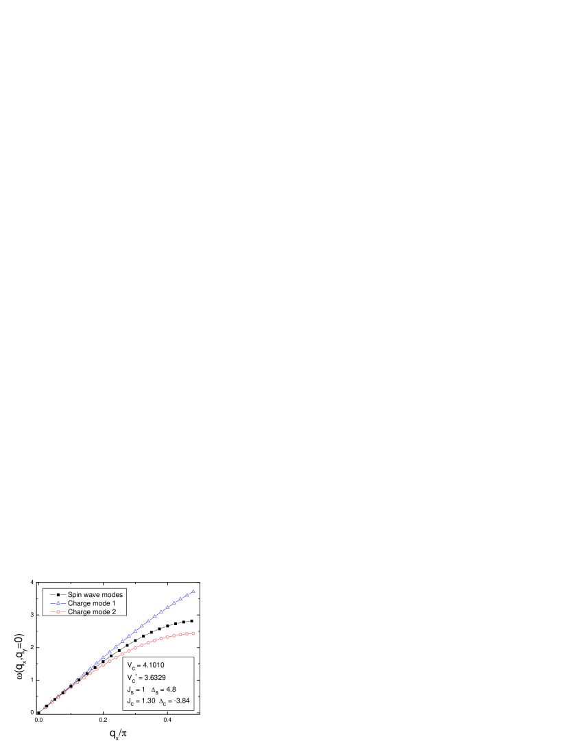
Figure 10: Dispersion of four gapless modes at a quantum multi-critical point, located tip of the $\delta=1/8$ checkerboard lobe illustrated in Fig. 6. The two spin wave modes have exactly the same dispersion due to the $SO(3)$ symmetry of AF moment. For the parameters shown in the figure, these four modes have the same speed at the multi-critical point. These four modes correspond the four Goldstone modes required by the quantum dynamical $SO(5)$ symmetry.

As one approaches the left part of the second order lobe following a trajectory with constant $J_{c}$, the energy cost of removing hole-pair decreases and becomes zero at the phase boundary. This observation leads to the conclusion that a particle-like charge mode becomes soft on the left part of the lobe. Similarly, one can argue that a hole-like charge mode becomes soft at the right part. At the tip, where the left part and right part of the lobe meet, both particle-like and hole-like modes become soft. Consequently, an effective particle-hole symmetry is dynamically restored. One can check that $C_{2}$ indeed vanishes at the tip of the lobe.

At the tip of the lobe, the speed of gapless charge modes is determined by the interaction $V_{c}$ and $V_{c}^{\prime}$. For appropriate values of $V_{c}$ and $V_{c}^{\prime}$, the speed of the gapless charge mode can be the same as the speed of the two gapless AF spin wave modes. When quantum $SO(5)$ symmetry is spontaneously broken to a $SO(4)$ symmetry, there should be exactly four degenerate gapless Goldstone bosons. This model shows that such a dynamical symmetry is possible at the multi-critical point around the tip of the $\delta=1/8$ lobe. Fig. 10 plots the dispersions of four gapless modes at the tip of AF insulating checkerboard lobe in the phase diagram of Fig. 6.

V Phase diagram obtained from Quantum Monte-Carlo simulation

V.1 Numerical simulation

Because of the bosonic nature, the minus-sign problem is absent in the quantum $SO(5)$ model. Therefore, simulations can be carried out for systems with sizes much larger than the ones available with fermionic QMC simulation in the physically interesting region. The pioneering numerical worksDorneich et al. (2002); Jöstingmeier et al. (unpublished); Hu (1999, 2001); Riera (2002a, b) show that the projected $SO(5)$ model can give a realistic description of the phase diagram of the HTSC cuprates and account for many of their physical properties. In this section, we shall present the simulation of the $SO(5)$ model with extended interactions using the Stochastic Series Expansion (SSE) method Sandvik and Kurkijarvi (1991); Sandvik (1997, 1999) with operator-loop update Sandvik (1999). This Quantum Monte Carlo method was shown to be very efficient for simulations of harcore bosonic systems Hebert et al. (2002); Schmid et al. (2002); Dorneich et al. (2002). The overall topology of the phase diagram agrees well with the mean field calculation presented in the previous section, although the parameters are strongly renormalized.

From the values given in section II, we see that we can safely neglect $J_{\pi}$ which is rather small so that only remains $J_{c}$ and $J_{s}$ which are both positive. In this section, $J_{\pi}=0$.

In order to avoid the notorious sign problem in the Quantum Monte Carlo simulations of the $SO(5)$ model with extended interactions, all off-diagonal terms should be positive. On a square lattice with only nearest-neighbour non-zero off-diagonal terms, the sign of these matrix elements can be safely changed by a harmless unitary transformation acting on hopping terms in only one of the sublattices.

For each simulation, the number of loops (or “worms”) made during the loop operator update Sandvik (1999) is calculated self consistently during the thermalization part, such that on average the number of vertices visited by worms during each loop operator update is equal to $C\langle n\rangle$. Here $\langle n\rangle$ is the average number of non-Identity vertices in the operator string (see Ref. [Sandvik, 1999]) and $C$ a proportionnality constant, usually taken between 1 and 5 (the larger $C$, the more autocorrelations between successive Monte Carlo configurations are reduced).

In order to plot the phase diagram, we should compute the order parameters corresponding to AF, SC and PDW phase.We use the superfluid density $\rho_{c}$ to locate SC phases. Indeed, $\rho_{c}$ can be related to the winding numbers of the world-lines which can be directly computed during the QMC simulations Pollock and Ceperley (1987); Sandvik (1997). Here the winding number only involves the charged particles, i.e. the hole pair hopping. We can take a similar definition with the magnetic bosons to define the spin stiffness.

It is straightforward to measure the density-density correlations and their Fourier transform, the structure factors $N(q_{x},q_{y})$ which indicate PDW phases :

$$N(\vec{q})=\frac{1}{L^{2}}\sum_{i,\vec{r}}exp(i\vec{q}.\vec{r})\langle n_{h}(i)n_{h}(i+\vec{r})\rangle$$

These quantities characterize the diagonal long-range order. On finite clusters, the structure factor at the appropriate momentum diverges as the volume of the system in the ordered phase, so that, by plotting $N(q_{x},q_{y})/L^{2}$ vs $1/L$ ($L$ is the linear size of the system), a scaling analysis can demonstrate long range order.

Due to the intrinsic complexity of the projected SO(5) model and to the large number of interaction types, we restricted the simulations to small lattices ($4\times 4$ up to $10\times 10$ lattices) at low temperatures (typically $\beta=10$), to mainly be in the ground state. Even using the powerful SSE method, we found that for specific points in the phase diagram (near phase boundaries for example), autocorrelation times of different observables or tunneling times between two neighbouring phases can be long, decreasing the statistical precision. This sometimes prevents us from providing definitive statements about the nature of phase transitions. However, outside of these regions, we can clearly distinguish the nature of the different phases.

V.2 Limiting cases

The pure projected SO(5) model corresponds to $V_{c}=V_{c}^{\prime}=V_{\pi}=0$ and $J_{c}=2J_{s}$. This model has been studied with the same technique Dorneich et al. (2002). A first-order transition between AF and SC phases was observed. It was already recognized that a small $V_{c}$ and $V_{c}^{\prime}$ were enough to turn this transition into a second-order phase transition.

Another interesting case occurs when the triplet density becomes small. In that limit, the model reduces to one type of hard-core boson with hopping $J_{c}$ and nearest and next-nearest neighbor repulsion $V_{c}$ and $V_{c}^{\prime}$ respectively.

$$H = -J_{c}\sum_{\langle ij\rangle}\left[t^{\dagger}_{h}(i)t_{h}(j)+H.c.\right]$$ (28)

$$+\left[V_{c}\sum_{\langle ij\rangle}+V_{c}^{\prime}\sum_{\langle\langle ij\rangle\rangle}\right]n_{h}(i)n_{h}(j)$$

so that we can fix $J_{c}=1$ as the energy unit. This model has been extensively studied in Ref. [Hebert et al., 2002] and some results have been obtained with the same SSE method. Let us review a few useful results.

V.2.1 Half-filling

The phase diagram at half-filling is well known and exhibits solid phases with either $(\pi,0)$ (stripe) or $(\pi,\pi)$ (checkerboard) structures. In between exists a superfluid phase with a non-zero superfluid density $\rho_{c}$. We recover the same results as Hebert et al. Hebert et al. (2002) : with our choice of interactions, by varying $J_{c}$, we can drive the system from a superfluid toward a $(\pi,0)$ (stripe) phase.

V.2.2 Away from half-filling

Away from half-filling, our grand-canonical algorithm is able to check whether we are in a phase separated state or not by looking at the histogram of the density during the simulation. On general grounds, the presence of a double peak structure shows the presence of true phase separation in the system.

With our choice of parameters, we find that away from the striped state, there is a phase, close to half-filling, where both $N(0,\pi)/L^{2}$ (PDW order parameter) and $\rho_{c}$ are finite, that is a supersolid phase. Moreover, there is no sign of phase separation so that it is a true homogeneous phase, as claimed in Ref. [Hebert et al., 2002].

V.3 Global phase diagram

Now that the parameters are fixed, we can compute the phase diagram for various $J_{c}$ and chemical potential $\Delta_{c}$ (see Fig. 11). In order to discuss these results, we plot in the following most of the data as a function of doping $\delta=n_{h}/2$ which depends on the chemical potential $\Delta_{c}$ as shown on Fig. 12, but has no strong finite-size effects. Let us comment on some results.

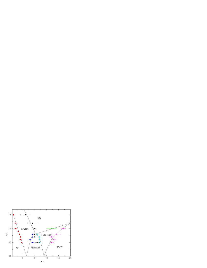
Figure 11: The global phase diagram obtained by QMC. The parameters used in simulation are $\Delta_{s}=4.8$, $V_{c}=4.1010$, $V_{c}^{\prime}=3.6329$ and $J_{\pi}=V_{\pi}=0$. The lines are guides to the eye only. The overall topology of the phase diagram agrees well with the mean-field phase diagram of Fig. 6, although the parameters are renormalized.

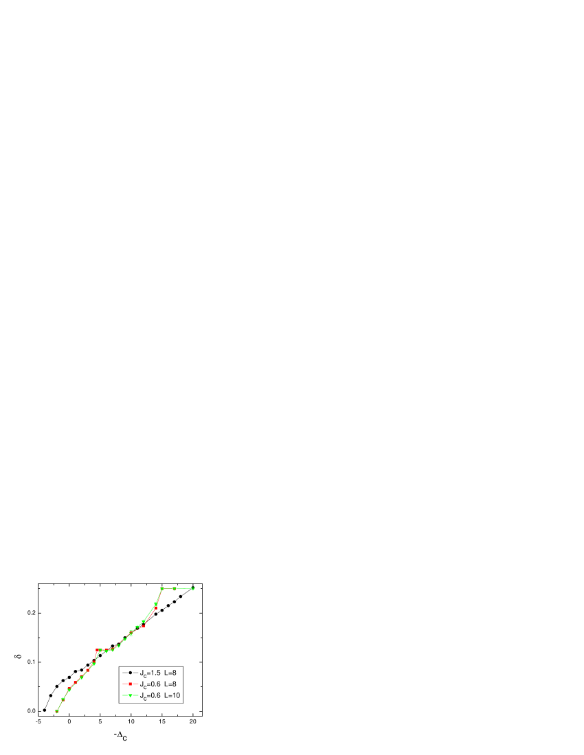
Figure 12: $\delta=n_{h}/2$ vs chemical potential for $J_{c}=1.5$ and $J_{c}=0.6$. The presence of plateaux indicates incompressible PDW phases. The finite size effects are rather small.

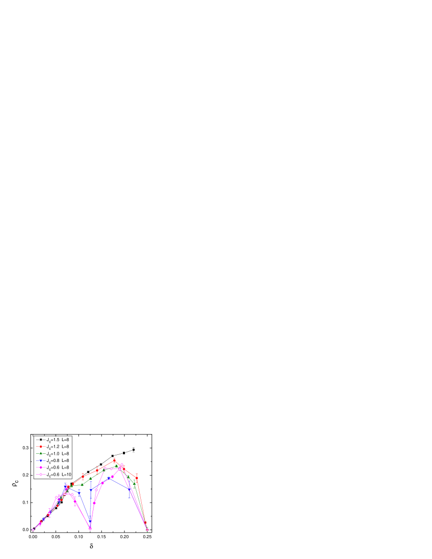
Figure 13: Superfluid density as a function of doping for various $J_{c}$. The “class B1” trace with $J_{c}=1.0$ bears great similarity with the famous dome-like phase diagram of many cuprate families. Also, the “class B3”-like trace with $J_{c}\leq 0.8$ has a pronounced dip at $\delta=1/8$ as the phase diagram of $LSCO$ family does.

V.3.1 Large $J_{c}$

For all values of $J_{c}$, the superfluid density increases linearly with doping, for small doping, thus capturing a key piece of the Mott physics. For large $J_{c}$ ($J_{c}=1.5$ for example), reducing hole density starting from $\delta=1/4$, we have a smooth decrease of superfluid density (see Fig. 13). At the same time, magnon density increases and gives rise to AF. Fig. 14 shows typical data of $N(\pi,0)/L^{2}$ which is the PDW order parameter for various sizes. In order to get information on the thermodynamic limit, we have performed a finite-size scaling of our data, and it vanishes for all fillings. We have a superconducting state for all dopings, with a possible coexistence with AF at low-doping. When the doping vanishes, we recover a pure AF phase.

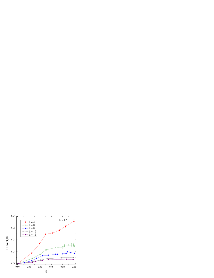
Figure 14: Scaling of $(\pi,0)$ PDW order parameter ($N(\pi,0)/L^{2}$) for various sizes ($L=6$ to 12 from top to bottom) with $J_{c}=1.5$. We checked that it extrapolates to 0 for all $\delta$.

V.3.2 Small $J_{c}$

For smaller $J_{c}$, the long-range interactions between hole pairs start to play a role.

Large doping — The first example is the appearance of a $(\pi,0)$ PDW insulating phase at $n_{h}=1/2$ ($\delta=1/4$). Indeed, close to this doping, the magnon density is very small so that the model is similar to the single hardcore boson case. We therefore recover a transition at fixed $n_{h}=1/2$ ($\delta=1/4$) as a function of $J_{c}$ between a superfluid phase (SC) and an insulating stripe phase (with a finite PDW order and a vanishing superfluid density). A finite-size scaling of the PDW order parameter showing a finite value is shown on Fig. 15 for $n_{h}=0.5$ ($\delta=0.25$) and $J_{c}=0.6$. On Fig. 13, we see that below $J_{c}\sim 1.3$, the superfluid density vanishes at $n_{h}=1/2$ ($\delta=1/4$) in agreement with what has been found for the single-boson model Hebert et al. (2002). Mean-field results find a higher value ($V_{c}^{\prime}/2\simeq 1.8$).

Intermediate doping — A second example of the interaction effect is given by the appearance of an insulating PDW phase at $n_{h}=0.25$ ($\delta=0.125$) for low enough $J_{c}$ ($J_{c}\leq 0.7$). A finite PDW order parameter and $\rho_{c}=0$ are shown again on Fig. 15 and 13 for $J_{c}=0.6$. This state corresponds to a localization of one hole-pair every 4 sites, so that this $n_{h}=1/4$ ($\delta=1/8$) checkerboard also possesses a finite $N(\pi,\pi)/L^{2}$ as shown on Fig. 16. We find that this $n_{h}=1/4$ ($\delta=1/8$) checkerboard is insulating, with a vanishing superfluid density. However, it could be possible to have a supersolid phaseTroyer .

For intermediate dopings $0.25<n_{h}<0.5(0.125<\delta<0.25)$ and small $J_{c}$, we find a finite superfluid density and possibly a finite PDW order, that is a supersolid region. We checked that this phase is stable against phase separation. We cannot be conclusive about its extension in the phase diagram, due to the long autocorrelation time for some observables. This explains the large error bars in some parts of the phase diagram. However, since we know that such a phase exists and is stable close to half-filling, we can assume that it has a finite extension. It would be interesting to check whether this supersolid also exists for a single hard-core boson model close to $n_{h}=1/4$ ($\delta=1/8$), which is much easier to simulate. It is remarkable that for $J_{c}$ values close to the transition, we see a dip in the superfluid density (Fig. 13), which is due to the proximity to the insulating state.

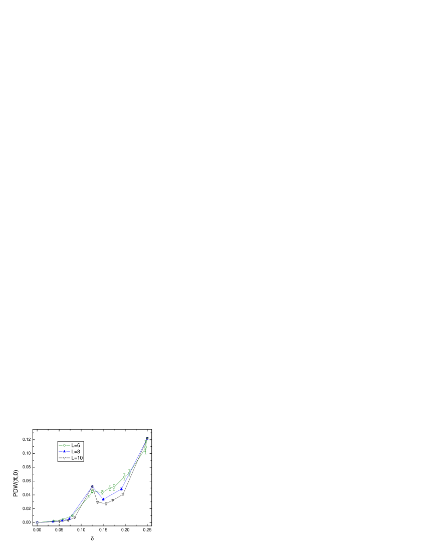
Figure 15: $(\pi,0)$ PDW order as a function of $\delta$ for various sizes ($L=6,8$ and $10$) for $Jc=0.6$. We checked that, within the system sizes simulated, finite PDW order survives in the thermodynamic limit for $n_{h}\geq 0.25$ ($\delta\geq 0.125$).

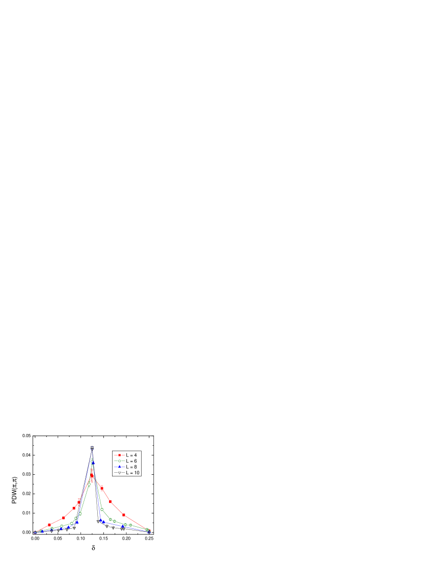
Figure 16: $(\pi,\pi)$ PDW order as a function of $\delta$ for various sizes ($L=4$, 6, 8 and 10) and $J_{c}=0.7$. We checked that it is finite only for $n_{h}=1/4$ ($\delta=1/8$) checkerboard.

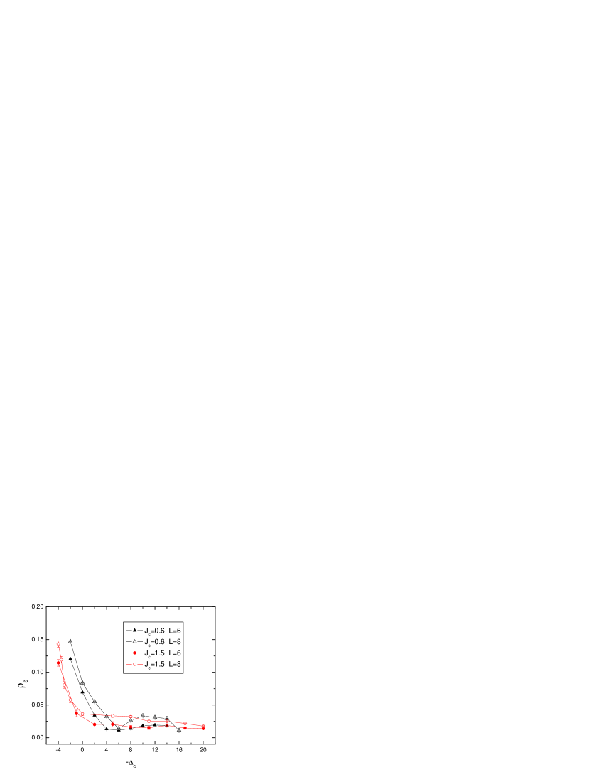
Figure 17: The spin stiffness versus chemical potential for different sizes and $J_{c}$.

V.3.3 Magnetic properties

As shown on Fig. 17, the spin stiffness shows a monotonic decrease with chemical potential (or doping) so that it is difficult to locate precisely where it vanishes. For small doping $\delta$ or chemical potential $-\Delta_{c}$, we observe a rapid linear decrease so that we can estimate roughly where AF could vanish in the thermodynamic limit. These phase boundaries are shown on Fig. 11 and are in agreement with what has been found at the mean-field level.

For small $J_{c}$, AF seems to vanish at $n_{h}=1/4$ ($\delta=1/8$). However, our data of $\rho_{s}$ also show a shallow peak above this filling, which could indicate a reentrance of AF as found in mean-field. Unfortunately, with our current limitation on available sizes and statistics, we cannot conclude for sure about this possibility.

V.4 Summary

The qualitative features found at the mean-field level are still present in a full numerical calculation and we have a very nice overall agreement (see Fig. 6 and 11). Of course, exact critical values of $J_{c}$ for superconducting-insulator transition are different from mean-field values but this does not change the physical conclusions.

It is very difficult to point precisely where AF vanishes since spin stiffness does not show any sharp drop. However, we clearly see a strong reduction of $\rho_{s}$, which seems to decrease linearly with doping. With the chosen parameters, it seems plausible that both this line and the PDW transition line merge close to the tip of the $n=1/4$ lobe as was found at the mean-field level. This result was associated to the dynamical restoration of $SO(5)$ symmetry at this point. Our data might be an indication that this is indeed the case (we have taken the same $V_{c}$ and $V_{c}^{\prime}$ so it seems pretty robust). However, a complete answer can only be provided by computing dynamical correlations, which is more involved and require good statistics.

VI Experimental consequence and predictions

In this work we have constructed a single quantum Hamiltonian based on the projected $SO(5)$ model with extended interactions, and presented detailed analytical and numerical calculations which give a consistent global phase diagram as depicted in Fig. 4. This schematic phase diagram is obtained from the quantitative model calculations summarized in Fig. 6 and 11. This model captures the overall topology of the cuprates phase diagram, including the dome-like feature of $T_{c}$, which is determined within our model by the superfluid density, the $1/8$ anomaly due to charge ordering, the coexistence of SC with AF and possibly with charge order. As mentioned in the introduction, some of these features have been discussed in other theoretical contexts before, however, it is rather remarkable that they are all reproduced by a single quantum model accessible by reliable QMC. Below we shall discuss some of these features and present more detailed theoretical predictions.

VI.1 Dependence of superfluid density on doping

A remarkable feature of the HTSC cuprates is the dome-like dependence of $T_{c}$ on doping. Experiments have also shown a remarkable dependence of superfluid density on doping. On the underdoped side, both $T_{c}$ and the superfluid density scales linearly with doping, a fact commonly referred to as the “Uemura plot”. Further examination also shows that the superfluid density in the overdoped regime decreases with increasing doping, which is commonly referred to as the “boomerang effect”. In cuprate system, the muon spin relaxation rate $\sigma(T\rightarrow 0)$ is proportional to $n_{s}/m^{*}$ where $n_{s}$ is the superfluid density and $m^{*}$ is the effective mass of hole-pairsUemura (2001). To explain the deviation from the linear relation between $\sigma$ and doping in the overdoped regime, Uemura proposed that some of the doped holes do not form pairs and are phase separated from the SC hole-pairs, even at zero temperatureUemura (2001). A similar phase separation picture was proposed by UchidaUchida (2003). However, it has always been rather puzzling that if the phase separated normal electrons existed at zero temperature, they should provide a channel of relaxations, which has not been observed experimentally.

Within our effective bosonic model, $T_{c}$ is directly determined by the superfluid density $\rho_{c}$. As we can see from Fig. 13, $\rho_{c}$ indeed scales linearly with the doping density for small doping, and has a dome-like dependence for higher doping for intermediate values of $J_{c}$. It peaks around $\delta\sim 18\%$ for $J_{c}=1.2$. The physical reason for the behavior on the overdoped side arises from the tendency of hole pairs to form a competing charge ordering state at either $3/16$ or $1/4$. Within this picture, when more holes are added into the system on the overdoped side, the holes are still paired, but some of them form a charge ordered PDW state, with preferred doping of $3/16$ or $1/4$. This charge ordered PDW state either phase separate from the SC state, or coexists with it, but either way, the superfluid density is reduced because of the repulsive coupling between the two forms of order. Therefore, this picture predicts a new charge ordered state on the overdoped side, which should be tested experimentally. Since the magnon density decreases monotonically with doping, the charge ordered states on the overdoped side may not be AF ordered, which makes it hard to observe by neutron scattering. Furthermore, on the overdoped side, our purely bosonic model also becomes less accurate, and a fully quantitative theory has to include the low energy fermionic excitations.

VI.2 The $1/8$ anomaly and pressure experiments

In the $LSCO$ systems, $T_{c}$ has a pronounced dip near doping of $\delta=1/8$Moodenbaugh et al. (1988). More recently, it has been demonstrated that the competition between the nearly insulating $1/8$ phase and the SC phase in $LSCO$ family can be controlled by pressure. There are two different approaches. One is to apply hydrostatic or uniaxial pressure on single crystalArumugam et al. (2002). In this way, the pressure in $ab$ plane increases $T_{c}$ while the pressure in $c$ direction decreases $T_{c}$. The other is to introduce compressive or expansive strain into thin films with the help of the lattice mismatch between the film and substrateSato et al. (2000). Enhanced $T_{c}$ and disappearance of the $1/8$ anomaly for compressed film and strong reduction of $T_{c}$ for expanded film were observedSato et al. (2000).

Our model reproduces the $\delta=1/8$ effect for $J_{c}<1$, as one can see from Fig. 13. The pronounced dip is caused from the competition between the SC state and the insulating PDW states. Varying doping correspond to the “B2” or “B3” traces as depicted in Fig. 4. On the other hand, pressure in the $ab$ plane reduces the lattice constant, thus increases the hopping term $J_{c}$. Therefore, applying pressure in the $ab$ plane is equivalent to following a “class A2” trace starting from a small $J_{c}$ in the global phase diagram. The doping dependence of $T_{c}$ for different films given in Fig. 3 of Sato et alSato et al. (2000) shares many common features with our doping dependence of SC order parameter, both MF results (Fig. 7) and QMC results (Fig. 13). The destructive effect on $T_{c}$ of the pressure in the $c$-direction can also be understood in terms of the Poisson effect. The lattice constant in $ab$ plane will increase when the sample is compressed in the $c$ direction. This will lead to the decrease of $T_{c}$ as argued previously.

Similar to the “class A2” trace, “class A3” trace can also be realized by applying pressure. Therefore, we predict a similar pressure induced superconductor-to-insulator transition at $\delta=1/16$.

In this way, the pressure effect on the $1/8$ anomaly is understood in terms of the bosonic superfluid-to-insulator transition at the fixed density of $\delta=1/8$. Standard predictions on the superfluid-to-insulator transition applies to the $\delta=1/8$ transition. In addition, we argued that the tip of the $\delta=1/8$ lobe can possibly have the full quantum $SO(5)$ symmetry. This prediction can be experimentally tested by comparing both the static and dynamic charge and magnetic responses, as we have discussed in section II.B.

VI.3 The vortex phase and the ground state above $H_{c2}$

The “class A2” and “class A3” traces can also be approached in the cuprates by applying a magnetic field along the $c$-axis, which effectively reduces the hopping term $J_{c}$. In underdoped $LSCO$ samples, we predict that the magnetic field destroys SC order by localizing hole-pairs into a PDW state. This naturally leads to the field-induced insulating behavior in underdoped $LSCO$Hawthorn et al. (2003); Sun et al. (2003). For the $YBCO$ and $BSCO$ systems, the magnetic field could drive the hole-pairs into a disordered state before the lobe of $\delta=1/8$ or $\delta=1/16$ is reached.

Recently, a striking feature is revealed in the STM experiments by Hoffman et al.Hoffman et al. (2002), where the local density of states (DOS) near the vortex core show a two dimensional checkerboard-like modulation with a $4a\times 4a$ charge unit cell. Here $a$ is the lattice spacing of the $CuO_{2}$ plane. This modulation decays exponentially away from the center of the vortex core, with a decay length of about $10a$. A similar pattern has also been seen in the absence of the applied magnetic fieldHowald et al. (2003), possibly induced by the impurities at the surface. In the case of vortex core experiment, SC is destroyed by the magnetic field, and the nature of the competing state is revealed. The case of impurity scattering is more complex, and the experimental observation can also be interpreted as due to quasi-particle interferenceWang and Lee (2003); McElroy et al. (2003a, b).

The $\delta=1/8$ insulating PDW state was proposed as an explanation for the STM measurementsChen et al. (2002). This state has the $4a\times 4a$ checkerboard symmetry as observed in the experiment, and the doping level for the insulating $\delta=1/8$ state is reasonably close to the optimal doping level of the cuprates. On the other hand, if the holes themselves, rather than the hole pairs, form a Wigner crystal state, the periodicity of the charge ordering would be larger by a factor of $\sqrt{2}$, inconsistent with the experiment. Therefore, by forming the Wigner crystal state of the hole pairs rather than the holes themselves, the doping level can be compatible with the observed size of the charge unit cell. In Ref.[Chen et al., 2002], the hole pair checkerboard state was established by a mean field calculation. A main result of the present work is to establish the existence of this state by QMC calculations.

Our calculations as summarized in Fig. 6 and 11 show that the charge ordered insulating states are also accompanied by AF magnetic order. Enhanced AF fluctuation in the vortex state was originally predicted within the $SO(5)$ theory in Ref.[ Zhang, 1997; Arovas et al., 1997], and has been experimentally observed in a number of HTSC cuprate families by a variety of experimental techniquesKatano et al. (2000); Mitrovic et al. (2001); Lake et al. (2001, 2002); Miller et al. (2002); Khaykovich et al. (2002); Mitrovic et al. (2003). More recently, AF order has been detected by neutron scattering above $H_{c2}$, in electron doped cupratesKang et al. (2003); Fujita et al. (unpublished). This magnetic field induced quantum phase transition from the SC state to the AF state correspond to the “A2” trace as depicted in Fig. 4.

VI.4 Charge localization and suppression of thermal conductivity

In previous subsections, we argue that the competition between PDW and SC can be tuned by applying pressure or magnetic field. In particular, we show that the PDW ordering of hole-pairs can develop in the vortex core. The localized hole-pairs in a PDW state are expected to have little contribution to the transport properties such as thermal conductivity. This leads to the argument of the suppression of thermal conductivity by applying a magnetic field in $c$-axis below some temperature $T_{K}$. Since the onset temperature $T_{K}$ is expected to be proportional to the superfluid density, $T_{K}$ has weak dependence on the magnetic field and follows $T_{c}$ in the underdoped cuprates. Moreover, the closer the system is to the charge ordered insulating state such as the $1/8$ PDW state, the smaller the suppression effect would be. Finally, the in-plane magnetic field has little effect on the thermal conductivity due to the fact that it does not create vortex in the $ab$ plane.

Therefore, trace “A2” in our global phase diagram and the charge localization into a hole pair crystal can possibly explain the recent experiment on the suppression of thermal conductivity by applying a magnetic field in $c$-directionKudo et al. (unpublished). We also predict that applying pressure will also induce the suppression or enhancement of the thermal conductivity around the $1/8$ doping, assuming the pressure will not induce strong effect of the lattice structure which can also change the thermal conductivity.

VI.5 1/16 doping

As discussed in section III, additional insulating lobes at $\delta=1/16$ and $\delta=3/16$ doping levels are predicted if interactions are more extended than the nnn interactions included in this work. The charge and spin ordering patterns for this state are depicted in Fig. 18. Even though the current paper does not investigate this type of more extended interactions explicitly due to numerical complexities, it is clear that the physics of these PDW states are similar to the $1/8$ doping. Preliminary evidence for the $\delta=1/16$ insulating state exists for the $LSCO$ materialKim and Hor (2001); Zhou et al. (unpublished). As we see from Fig. 18 and 19, the charge ordering pattern rotates from diagonal at $\delta=1/16$ to square at $\delta=1/8$. This transition between states with different rotational symmetries could possibly be related to the diagonal to square transition observed in the neutron scattering experiments at $\delta\sim 5\%$ in the $LSCO$ materialFujita et al. (2002); Matsuda et al. (2000).

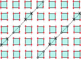
Figure 18: The hole-pair checkerboard state with anti-phase magnetic domain at doping level $\delta=1/16$. Circles denote holes and arrows denote spins while black crosses denote spins in a singlet bond.

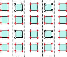
Figure 19: The hole-pair checkerboard state with in-phase magnetic domain at doping level $\delta=1/8$. Circles denote holes and arrows denote spins while black crosses denote spins in a singlet bond.

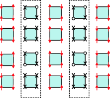
Figure 20: The hole-pair checkerboard state with anti-phase magnetic domain at doping level $\delta=1/8$. Circles denote holes and arrows denote spins while black crosses denote spins in a singlet bond.

VI.6 Magnetic order

In this paper, we focused our discussion on the checkerboard charge order at $\delta=1/8$. Strictly within our model, the accompanied AF magnetic order is commensurate, as sketched in Fig. 19. This type of magnetic structure is consistent with the recently observed field induced magnetic order in the $NCCO$ materialKang et al. (2003); Fujita et al. (unpublished), but not consistent with the magnetic structure observed in the $LSCO$ material, which has anti-phase domain walls. We would like to stress that this is not a limitation on the fundamental approach taken here. As shown in Fig. 20, checkerboard charge order of the hole pairs can be fully consistent with the AF magnetic structure with anti-phase domain walls. However, stability of this type of magnetic structure requires more extended magnetic interactions. Since the complexity of both the CORE algorithm and the QMC increases substantially, we have not yet been able to derive such extended interactions from the microscopic models, and simulate them with QMC.

VI.7 Coexistence phases

While the simple $SO(5)$ modelZhang (1997) predicts the coexistence phases of AF and SC, more regions with coexisting charge, AF and SC orders are predicted in the global phase diagram of Fig. 6 and Fig. 11. In particular, the “type 1” first order transition from undoped AF state to SC state predicted by simple $SO(5)$ model is turned into two “type 2” second order transitions by the interactions $V_{c}$ and $V_{c}^{\prime}$, which is consistent with previous studyDorneich et al. (2002). While the width of these coexistence regions is model dependent, coexistence phases are important qualitative predictions of our theory. Experiments on cuprates have indeed suggested such coexistence phasesBrewer et al. (1989); Niedermayer et al. (1998); Sonier et al. (2001); Sidis et al. (2001); Mook et al. (2002); Miller et al. .

As we see from Fig. 8, the AF order disappears around $\delta=0.10$. This is consistent with the value obtained from the $t$-$J$ modelHimeda and Ogata (1999). The width of the AF/SC coexistence phase largely depends on the values of $J_{\pi}$ and $V_{\pi}$. As determined by CORE method, $J_{\pi}$ is negative and $V_{\pi}$ is positive. Thus, at the mean-field level, both $J_{\pi}$ and $V_{\pi}$ terms induce a repulsion between AF and SC in the mixed state of coexisting AF and SC. When these terms are included, one would expect a smaller region of the AF/SC coexistence state of in the global phase diagram. On the other hand, these two terms have different effects on the checkerboard state. Since the mean-field value of $\pi$-operator in the PDW state is zero, the $J_{\pi}$ interaction will not induce any interaction terms at the mean-field level. In contrast, the $V_{\pi}$ term effectively changes the local chemical potential of hole-pairs (magnons) due to the nonzero mean-field value of magnons (hole-pairs) on nn plaquette. Therefore, $V_{\pi}$ also reduces the height of the insulating PDW lobe.

VII Conclusions

Starting from commonly used microscopic models of high $T_{c}$ cuprates, an effective bosonic model can be derived by the CORE algorithmAltman and Auerbach (2002); Capponi and Poilblanc (2002). In addition to the simple interactions included in the original projected $SO(5)$ modelZhang et al. (1999); Dorneich et al. (2002); Jöstingmeier et al. (unpublished), extended interactions play an important role in determining the global phase diagram of the model. This model can be studied systematically by the analytical mean field theory and by the QMC method, thanks to the absence of the minus sign problem. The global phase diagram consists of self-similar insulating PDW phases at rational filling fractions, immersed in the background of the uniform SC phase, as depicted schematically in Fig. 4. Different families of cuprates are attributed to different traces in the global phase diagram. The overall topology of the phase diagram obtained from our model agrees well with the experiments, and so are the behaviors of various physical quantities. Inclusion of longer ranged interactions could bring detailed and quantitative agreements with the cuprate phase diagram.

VIII acknowledgments

We would like to acknowledge useful discussions with Drs. A. Auerbach, E. Demler, W. Hanke, J.P. Hu, S. Kivelson, E. Mukamel, G. Schmid, M. Troyer and C.J. Wu. This work is supported by the NSF under grant numbers DMR-9814289, and the US Department of Energy, Office of Basic Energy Sciences under contract DE-AC03-76SF00515 and by the Swiss National Science Foundation. HDC is also supported by a Stanford Graduate Fellowship. Part of the simulations were performed on the Asgard beowulf cluster at ETH Zürich and at SLAC.

References

- Zhang (1997) S. C. Zhang, Science 275, 1089 (1997).
- Demler and Zhang (1995) E. Demler and S. C. Zhang, Phys. Rev. Lett. 75, 4126 (1995).
- Demler and Zhang (1998) E. Demler and S. C. Zhang, Nature 396, 733 (1998).
- Rossatmignod et al. (1991) J. Rossatmignod, L. P. Regnault, C. Vettier, P. Bourges, P. Burlet, J. Bossy, J. Y. Henry, and G. Lapertot, Physica C 185, 86 (1991).
- Mook et al. (1993) H. A. Mook, M. Yethiraj, G. Aeppli, T. E. Mason, and T. Armstrong, Phys. Rev. Lett. 70, 3490 (1993).
- Fong et al. (1995) H. F. Fong, B. Keimer, P. W. Anderson, D. Reznik, F. Dogan, and I. A. Aksay, Phys. Rev. Lett. 75, 316 (1995).
- Dai et al. (1996) P. Dai, M. Yethiraj, H. A. Mook, T. B. Lindemer, and F. Dogan, Phys. Rev. Lett. 77, 5425 (1996).
- Fong et al. (1996) H. F. Fong, B. Keimer, D. Reznik, D. L. Milius, and I. A. Aksay, Phys. Rev. B 54, 6708 (1996).
- Mook et al. (1998) H. A. Mook, P. C. Dai, S. M. Hayden, G. Aeppli, T. G. Perring, and F. Dogan, Nature 395, 580 (1998).
- Dai et al. (1998) P. C. Dai, H. A. Mook, and F. Dogan, Phys. Rev. Lett. 80, 1738 (1998).
- Fong et al. (2000) H. F. Fong, P. Bourges, Y. Sidis, L. P. Regnault, J. Bossy, A. Ivanov, D. L. Milius, I. A. Aksay, and B. Keimer, Phys. Rev. B 61, 14773 (2000).
- Fong et al. (1999) H. F. Fong, P. Bourges, Y. Sidis, L. P. Regnault, A. Ivanov, G. D. Gu, N. Koshizuka, and B. Keimer, Nature 398, 588 (1999).
- He et al. (2001) H. He, Y. Sidis, P. Bourges, G. D. Gu, A. Ivanov, N. Koshizuka, B. Liang, C. T. Lin, L. P. Regnault, E. Schoenherr, et al., Phys. Rev. Lett. 86, 1610 (2001).
- He et al. (2002) H. He, P. Bourges, Y. Sidis, C. Ulrich, L. P. Regnault, S. Pailhes, N. S. Berzigiarova, N. N. Kolesnikov, and B. Keimer, Science 295, 1045 (2002).
- Stock et al. (unpublished) C. Stock, W. J. L. Buyers, R. Liang, D. Peets, Z. Tun, D. Bonn, W. H. Hardy, and R. J. Birgeneau, Phys. Rev. B 69, 014502 (2004).
- Tranquada et al. (unpublished) J. M. Tranquada, C. H. Lee, K. Yamada, Y. S. Lee, L. P. Regnault, and H. W. Ronnow, Phys. Rev. B 69, 174507 (2004).
- Arovas et al. (1997) D. P. Arovas, A. J. Berlinsky, C. Kallin, and S. C. Zhang, Phys. Rev. Lett. 79, 2871 (1997).
- Katano et al. (2000) S. Katano, M. Sato, K. Yamada, T. Suzuki, and T. Fukase, Phys. Rev. B 62, 14677 (2000).
- Mitrovic et al. (2001) V. F. Mitrovic, E. E. Sigmund, M. Eschrig, H. N. Bachman, W. P. Halperin, A. P. Reyes, P. Kuhns, and W. G. Moulton, Nature 413, 501 (2001).
- Lake et al. (2001) B. Lake, G. Aeppli, K. N. Clausen, D. F. McMorrow, K. Lefmann, N. E. Hussey, N. Mangkorntong, M. Nohara, H. Takagi, T. E. Mason, et al., Science 291, 1759 (2001).
- Lake et al. (2002) B. Lake, H. M. Ronnow, N. B. Christensen, G. Aeppli, K. Lefmann, D. F. McMorrow, P. Vorderwisch, P. Smeibidl, N. Mangkorntong, T. Sasagawa, et al., Nature 415, 299 (2002).
- Miller et al. (2002) R. I. Miller, R. F. Kiefl, J. H. Brewer, J. E. Sonier, J. Chakhalian, S. Dunsiger, G. D. Morris, A. N. Price, D. A. Bonn, W. H. Hardy, et al., Phys. Rev. Lett. 88, 137002 (2002).
- Khaykovich et al. (2002) B. Khaykovich, Y. S. Lee, R. W. Erwin, S. H. Lee, S. Wakimoto, K. J. Thomas, M. A. Kastner, and R. J. Birgeneau, Phys. Rev. B 66, 014528 (2002).
- Mitrovic et al. (2003) V. F. Mitrovic, E. E. Sigmund, W. P. Halperin, A. P. Reyes, P. Kuhns, and W. G. Moulton, Phys. Rev. B 67, 220503 (2003).
- Kang et al. (2003) H. J. Kang, P. C. Dai, J. W. Lynn, M. Matsuura, J. R. Thompson, S. C. Zhang, D. N. Argyriou, Y. Onose, and Y. Tokura, Nature 423, 522 (2003).
- Fujita et al. (unpublished) M. Fujita, A. Matsuda, S. Katano, and K. Yamada, cond-mat/0311269 (unpublished).
- Zhang et al. (1999) S. C. Zhang, J. P. Hu, E. Arrigoni, W. Hanke, and A. Auerbach, Phys. Rev. B 60, 13070 (1999).
- Altman and Auerbach (2002) E. Altman and A. Auerbach, Phys. Rev. B 65, 104508 (2002).
- Capponi and Poilblanc (2002) S. Capponi and D. Poilblanc, Phys. Rev. B 66, 180503 (2002).
- Dorneich et al. (2002) A. Dorneich, W. Hanke, E. Arrigoni, M. Troyer, and S. C. Zhang, Phys. Rev. Lett. 88, 057003 (2002).
- Riera (2002a) J. A. Riera, Phys. Rev. B 66, 134523 (2002a).
- Riera (2002b) J. A. Riera, Phys. Rev. B 65, 174526 (2002b).
- Jöstingmeier et al. (unpublished) M. Jöstingmeier, E. Arrigoni, W. Hanke, and S.-C. Zhang, Phys. Rev. B 68, 245111 (2003).
- Tranquada et al. (1995) J. M. Tranquada, B. J. Sternlieb, J. D. Axe, Y. Nakamura, and S. Uchida, Nature 375, 561 (1995).
- Aeppli et al. (1997) G. Aeppli, T. E. Mason, S. M. Hayden, H. A. Mook, and J. Kulda, Science 278, 1432 (1997).
- Wells et al. (1997) B. O. Wells, Y. S. Lee, M. A. Kastner, R. J. Christianson, R. J. Birgeneau, K. Yamada, Y. Endoh, and G. Shirane, Science 277, 1067 (1997).
- Hoffman et al. (2002) J. E. Hoffman, E. W. Hudson, K. M. Lang, V. Madhavan, H. Eisaki, S. Uchida, and J. C. Davis, Science 295, 466 (2002).
- Howald et al. (2003) C. Howald, H. Eisaki, N. Kaneko, M. Greven, and A. Kapitulnik, Phys. Rev. B 67, 014533 (2003).
- McElroy et al. (2003a) K. McElroy, R. W. Simmonds, J. E. Hoffman, D. H. Lee, J. Orenstein, H. Eisaki, S. Uchida, and J. C. Davis, Nature 422, 592 (2003a).
- Wang and Lee (2003) Q. H. Wang and D. H. Lee, Phys. Rev. B 67, 020511 (2003).
- McElroy et al. (2003b) K. McElroy, J. E. Hoffman, D. H. Lee, K. M. Lang, H. Eisaki, S. Uchida, and J. C. Davis, Physica C 388, 225 (2003b).
- Kivelson et al. (2003) S. A. Kivelson, I. P. Bindloss, E. Fradkin, V. Oganesyan, J. M. Tranquada, A. Kapitulnik, and C. Howald, Rev. Mod. Phys. 75, 1201 (2003).
- Chen et al. (2002) H. D. Chen, J. P. Hu, S. Capponi, E. Arrigoni, and S. C. Zhang, Phys. Rev. Lett. 89, 137004 (2002).
- Kivelson et al. (1992) S. Kivelson, D. H. Lee, and S. C. Zhang, Phys. Rev. B 46, 2223 (1992).
- Pryadko and Zhang (1996) L. P. Pryadko and S. C. Zhang, Phys. Rev. B 54, 4953 (1996).
- Burgess and Dolan (2001) C. P. Burgess and B. P. Dolan, Phys. Rev. B 63, 155309 (2001).
- Witten (unpublished) E. Witten, hep-th/0307041 (unpublished).
- Chen et al. (unpublished) H. Chen, O. Vafek, A. Yazdani, and S. Zhang, cond-mat/0402323 (unpublished).
- Zaanen and Gunnarsson (1989) J. Zaanen and O. Gunnarsson, Phys. Rev. B 40, 7391 (1989).
- Tsunetsugu et al. (1995) H. Tsunetsugu, M. Troyer, and T. M. Rice, Phys. Rev. B 51, 16456 (1995).
- Kivelson et al. (1998) S. A. Kivelson, E. Fradkin, and V. J. Emery, Nature 393, 550 (1998).
- White and Scalapino (1998) S. R. White and D. J. Scalapino, Phys. Rev. Lett. 80, 1272 (1998).
- Zaanen (1999) J. Zaanen, Science 286, 251 (1999).
- Emery and Kivelson (1995) V. J. Emery and S. A. Kivelson, Nature 374, 434 (1995).
- Vojta and Sachdev (1999) M. Vojta and S. Sachdev, Phys. Rev. Lett. 83, 3916 (1999).
- Demler et al. (2001) E. Demler, S. Sachdev, and Y. Zhang, Phys. Rev. Lett. 87, 067202 (2001).
- Zhang et al. (2002) Y. Zhang, E. Demler, and S. Sachdev, Phys. Rev. B 66, 094501 (2002).
- Laughlin (unpublished) R. B. Laughlin, cond-mat/0209269 (unpublished).
- Haas et al. (1995) S. Haas, E. Dagotto, A. Nazarenko, and J. Riera, Phys. Rev. B 51, 5989 (1995).
- Kim and Hor (2001) Y. H. Kim and P. H. Hor, Mod. Phys. Lett. B 15, 497 (2001).
- Fisher et al. (1989) M. P. A. Fisher, P. B. Weichman, G. Grinstein, and D. S. Fisher, Phys. Rev. B 40, 546 (1989).
- Pich and Frey (1998) C. Pich and E. Frey, Phys. Rev. B 57, 13712 (1998).
- Hebert et al. (2002) F. Hebert, G. G. Batrouni, R. T. Scalettar, G. Schmid, M. Troyer, and A. Dorneich, Phys. Rev. B 65, 014513 (2002).
- Morningstar and Weinstein (1996) C. J. Morningstar and M. Weinstein, Phys. Rev. D 54, 4131 (1996).
- Chakravarty et al. (1988) S. Chakravarty, B. I. Halperin, and D. R. Nelson, Phys. Rev. Lett. 60, 1057 (1988).
- Manousakis (1991) E. Manousakis, Rev. Mod. Phys. 63, 1 (1991).
- Vanotterlo and Wagenblast (1994) A. Vanotterlo and K. H. Wagenblast, Physical Review Letters 72, 3598 (1994).
- Batrouni et al. (1995) G. G. Batrouni, R. T. Scalettar, G. T. Zimanyi, and A. P. Kampf, Physical Review Letters 74, 2527 (1995).
- Kosterlitz et al. (1976) J. M. Kosterlitz, D. R. Nelson, and M. E. Fisher, Phys. Rev. B 13, 412 (1976).
- Arumugam et al. (2002) S. Arumugam, N. Mori, N. Takeshita, H. Takashima, T. Noda, H. Eisaki, and S. Uchida, Phys. Rev. Lett. 88, 247001 (2002).
- Sato et al. (2000) H. Sato, A. Tsukada, M. Naito, and A. Matsuda, Phys. Rev. B 62, R799 (2000).
- Hawthorn et al. (2003) D. G. Hawthorn, R. W. Hill, C. Proust, F. Ronning, M. Sutherland, E. Boaknin, C. Lupien, M. A. Tanatar, J. Paglione, S. Wakimoto, et al., Phys. Rev. Lett. 90, 197004 (2003).
- Sun et al. (2003) X. F. Sun, S. Komiya, J. Takeya, and Y. Ando, Phys. Rev. Lett. 90, 117004 (2003).
- Hu (1999) X. Hu, J. Low Temp. Phys. 117, 289 (1999).
- Hu (2001) X. Hu, Phys. Rev. Lett. 87, 057004 (2001).
- Sandvik and Kurkijarvi (1991) A. W. Sandvik and J. Kurkijarvi, Phys. Rev. B 43, 5950 (1991).
- Sandvik (1997) A. W. Sandvik, Phys. Rev. B 56, 11678 (1997).
- Sandvik (1999) A. W. Sandvik, Phys. Rev. B 59, 14157 (1999).
- Schmid et al. (2002) G. Schmid, S. Todo, M. Troyer, and A. Dorneich, Phys. Rev. Lett. 88, 167208 (2002).
- Pollock and Ceperley (1987) E. L. Pollock and D. M. Ceperley, Phys. Rev. B 36, 8343 (1987).
- (81) M. Troyer, private communication.
- Uemura (2001) Y. J. Uemura, Solid State Commun. 120, 347 (2001).
- Uchida (2003) S. Uchida, Solid State Commun. 126, 57 (2003).
- Moodenbaugh et al. (1988) A. R. Moodenbaugh, Y. W. Xu, M. Suenaga, T. J. Folkerts, and R. N. Shelton, Phys. Rev. B 38, 4596 (1988).
- Kudo et al. (unpublished) K. Kudo, M. Yamazaki, T. Kawamata, T. Adachi, T. Noji, Y. Koike, T. Nishizaki, and N. Kobayashi, cond-mat/0311402 (unpublished).
- Zhou et al. (unpublished) F. Zhou, P. H. Hor, X. L. Dong, W. X. Ti, J. W. Xiong, and Z. X. Zhao, cond-mat/0309034 (unpublished).
- Fujita et al. (2002) M. Fujita, K. Yamada, H. Hiraka, P. M. Gehring, S. H. Lee, S. Wakimoto, and G. Shirane, Phys. Rev. B 65, 064505 (2002).
- Matsuda et al. (2000) M. Matsuda, M. Fujita, K. Yamada, R. J. Birgeneau, M. A. Kastner, H. Hiraka, Y. Endoh, S. Wakimoto, and G. Shirane, Phys. Rev. B 62, 9148 (2000).
- Brewer et al. (1989) J. H. Brewer, J. F. Carolan, W. N. Hardy, B. X. Yang, P. Schleger, R. Kadono, J. R. Kempton, R. F. Kiefl, S. R. Kreitzman, G. M. Luke, et al., Physica C 162, 33 (1989).
- Niedermayer et al. (1998) C. Niedermayer, C. Bernhard, T. Blasius, A. Golnik, A. Moodenbaugh, and J. I. Budnick, Phys. Rev. Lett. 80, 3843 (1998).
- Sonier et al. (2001) J. E. Sonier, J. H. Brewer, R. F. Kiefl, R. I. Miller, G. D. Morris, C. E. Stronach, J. S. Gardner, S. R. Dunsiger, D. A. Bonn, W. N. Hardy, et al., Science 292, 1692 (2001).
- Sidis et al. (2001) Y. Sidis, C. Ulrich, P. Bourges, C. Bernhard, C. Niedermayer, L. P. Regnault, N. H. Andersen, and B. Keimer, Phys. Rev. Lett. 86, 4100 (2001).
- Mook et al. (2002) H. A. Mook, P. C. Dai, S. M. Hayden, A. Hiess, J. W. Lynn, S. H. Lee, and F. Dogan, Phys. Rev. B 66, 144513 (2002).
- (94) R. I. Miller, R. F. Kiefl, J. H. Brewer, J. E. Sonier, D. A. Bonn, W. H. Hardy, R. Liang, J. M. Mnard, and P. Poon, unpublished.
- Himeda and Ogata (1999) A. Himeda and M. Ogata, Phys. Rev. B 60, R9935 (1999).