Solitons and Rabi Oscillations in a Time-Dependent BCS Pairing Problem

Abstract

Motivated by recent efforts to achieve cold fermions pairing near a Feshbach resonance, we consider the dynamics of formation of the Bardeen-Cooper-Schrieffer (BCS) state. At times shorter than the quasiparticle energy relaxation time, after the interaction is turned on, the dynamics of the system is nondissipative. We show that this collective nonlinear evolution of the BCS-Bogoliubov amplitudes $u_{p}$, $v_{p}$, along with the pairing function $\Delta$, is an integrable dynamical problem, and obtain a family of exact solutions in the form of single solitons and soliton trains. We interpret the collective oscillations as Bloch precession of Anderson pseudospins, where each soliton causes a pseudospin $2\pi$ Rabi rotation. Numerical simulations demonstrate robustness of the solitons with respect to noise and damping.

Dilute fermionic alkali gases cooled below degeneracy [1] are expected to host the paired BCS state [2, 3]. One of the unique and attractive features of this system which makes it qualitatively different from superconducting metals is the possibility to control the strength of pairing interaction and change it by using the Feshbach resonances [4, 5, 6, 7, 8, 9]. Pairing enhancement near the resonances, as well as the high coherence of atomic systems, can allow to realize the strong coupling BCS regime, as well as to explore the time dynamics of the paired state. Since the characteristic energy scales in atomic vapors are relatively low, one can perform time-resolved measurements on the intrinsic microscopic time scales, and explore a range of fundamentally new phenomena in the time dynamics of the paired state. These new prospects helped to revive interest in some of the basic issues of the BCS pairing problem [10, 11, 12, 13, 14, 15].

In particular, one of the important questions has to do with the dynamics and characteristic times of formation of the BCS state in cold gases [16]. The dynamics of the superconducting state in metals, described by BCS theory, has been a subject of active research for a long time [17]. Generally, there are two important time scales to be considered: the quasiparticle energy relaxation time $\tau_{\epsilon}$, and the characteristic time of the order parameter change, $\tau_{\Delta}$, estimated as the inverse increment of Cooper instability [18, 19]. For $\tau_{\epsilon}\ll\tau_{\Delta}$, quasiparticles quickly reach local equilibrium parameterized by a time-dependent order parameter $\Delta(t)$. In this case the dynamics is described by the time-dependent Ginzburg-Landau (TDGL) equation for $\Delta(t)$, with the relaxation time scale ca. $\tau_{\Delta}$. However, as noted by Gorkov and Eliashberg [20], this scenario applies only to relatively exotic situations, including a close proximity of a transition point, $\Delta^{2}/T_{c}\ll\tau^{-1}_{\epsilon}$, or a fast pair breaking (e.g., due to paramagnetic impurities).

In the opposite limit, which takes place at the temperatures not too close to critical,

$$\tau_{\epsilon}\gg\tau_{\Delta}$$ (1)

the system dynamics is usually described by Boltzmann kinetic equation for quasiparticles and a self-consistent equation for $\Delta(t)$ connecting it with the quasiparticle distribution function locally in time [21, 22]. The validity of this approach requires, in addition to (1), that the variation in time of both the quasiparticle distribution and the external parameters is sufficiently slow on the $\tau_{\Delta}$ time scale. The origin of this criterion is seen most easily if one notes that the order parameter can exhibit free oscillations with a frequency ca. $\tau_{\Delta}^{-1}$ [23] (also, see below). Thus, at a slow parameter variation the order parameter $\Delta(t)$ and the quasiparticle spectrum will adiabatically follow the changes of the quasiparticle distribution, without exciting the oscillations of $\Delta$. This approximation is relevant to the majority of situations in superconducting metals because of the relatively big value of $\Delta$ and the difficulty of changing the external parameters and making measurements on the time scale of $\tau_{\Delta}$.

From this point of view, the cold fermionic gases present a completely new situation. The energy relaxation in these systems is quite slow, while the external parameters, such as the detuning from Feshbach resonance, can change very quickly on the time scale of $\tau_{\Delta}$. Thus the BCS correlations in this case build up in a coherent fashion while the system is out of thermal equilibrium. In such a situation, theory must account not only for the order parameter evolution, but also for the full dynamics of individual Cooper pairs and quasiparticles. It seems to be desirable to understand better this ‘fast BCS buildup’ regime, since the lifetime of the gas samples is finite, while the time-resolved measurements can easily be performed with resolution better than $\tau_{\Delta}$.

In this article we consider the situation when the pairing interaction is switched on essentially instantly, on a time scale $\tau_{0}\ll\tau_{\Delta},\tau_{\epsilon}$. We shall discuss only the spatially uniform situation, relevant for samples of finite size, and explore the time evolution of the unpaired ideal Fermi gas, which is unstable with respect to Cooper pairing. At not too long times, $t\ll\tau_{\epsilon}$, the dynamics of the system is governed by nondissipative equations which conserve both the entropy and the total energy. A stationary superconducting state with the same energy as that of the initial state would have more quasiparticles, and thus would have entropy higher than the initial Fermi gas entropy. This argument suggests that the system can reach a stationary (not necessarily equilibrium) state only at a very long time of the order $\tau_{\epsilon}$. On shorter times, which nevertheless can exceed $\tau_{\Delta}$), the system will exhibit a nonlinear time evolution. During this period of time the concept of the quasiparticle spectrum is irrelevant and theory can rely neither on the kinetic equation, nor on TDGL equation. Below, we present an approach which describes the BCS state buildup and accounts for coherent dynamics of individual Cooper pairs. We shall focus on the zero temperature case, when $\tau_{\Delta}\simeq\Delta^{-1}$, and show that the result of Cooper instability is a periodic oscillation $\Delta(t)$ having the form of a soliton train.

This regime can be described by the BCS hamiltonian

$${\cal H}=\sum_{{\bf p},\,\sigma}\epsilon_{{\bf p}}a^{+}_{{\bf p},\sigma}a_{{\bf p},\sigma}-\frac{\lambda(t)}{2}\sum_{{\bf p},{\bf q}}a^{+}_{{\bf p}\,\uparrow}a^{+}_{-{\bf p}\,\downarrow}a_{-{\bf q}\,\downarrow}a_{{\bf q}\,\uparrow}\,,$$ (2)

with the coupling turned on abruptly, $\lambda(t)=\lambda\theta(t-t_{\ast})$.

The main result of this work is that the time-dependent problem (2) is integrable. We generalize the BCS solution, which is exact for the separable pairing Hamiltonian (2), and demonstrate that at $t>t_{\ast}$ the many-body state evolves as

$$|\Psi(t)\rangle=\prod_{{\bf p}}\left(u_{{\bf p}}(t)+v_{{\bf p}}(t)a^{+}_{{\bf p},\uparrow}a^{+}_{-{\bf p},\downarrow}\right)|0\rangle$$ (3)

The Bogoliubov mean field treatment, which gives a state of the form (3), relies on the ‘infinite range’ form of the pairing interaction in (2) (i.e., equal coupling strength of all $({\bf p},-{\bf p})$, $({\bf q},-{\bf q})$). Since the latter does not depend on the system being in equilibrium, one can introduce a time-dependent mean field pairing function

$$\Delta(t)=\lambda\sum_{{\bf p}}u_{{\bf p}}(t)v_{{\bf p}}^{\ast}(t)$$ (4)

The amplitudes $u_{{\bf p}}(t)$, $v_{{\bf p}}(t)$ can be obtained from the Bogoliubov-deGennes equation

$$i\partial_{t}\left(\matrix{u_{{\bf p}}\cr v_{{\bf p}}}\right)=\left(\matrix{\epsilon_{{\bf p}}&\Delta\cr\Delta^{\ast}&-\epsilon_{{\bf p}}}\right)\left(\matrix{u_{{\bf p}}\cr v_{{\bf p}}}\right)$$ (5)

to be solved along with the selfconsistency condition (4).

We recall that the unpaired state is a selfconsistent, albeit unstable, solution of Eqs. (5),(4) with $\Delta=0$, $T=0$: $u^{(0)}_{{\bf p}}(t)=e^{-i\epsilon_{{\bf p}}t}\theta(\epsilon_{{\bf p}})$, $v^{(0)}_{{\bf p}}(t)=e^{i\epsilon_{{\bf p}}t}\theta(-\epsilon_{{\bf p}})$, The stability analysis [19] shows that the deviation from the unpaired state grows as $\Delta(t)\propto e^{\gamma t}e^{-i\omega t}$,

$$\delta u_{{\bf p}}(t)=\frac{\Delta(t)v^{(0)}_{{\bf p}}(t)}{i\gamma-2\epsilon_{{\bf p}}+\omega},\quad\delta v_{{\bf p}}(t)=\frac{\Delta^{\ast}(t)u^{(0)}_{{\bf p}}(t)}{i\gamma+2\epsilon_{{\bf p}}-\omega}$$ (6)

with the growth exponent $\gamma$ and the constant $\omega$ given by

$$1=\lambda\sum_{{\bf p}}\frac{{\rm sgn}\,\epsilon_{{\bf p}}}{2\epsilon_{{\bf p}}-\zeta},\quad\zeta=\omega+i\gamma$$ (7)

The electron-hole symmetry near the Fermi level, $N(\epsilon_{{\bf p}})=N(-\epsilon_{{\bf p}})$, makes the frequency shift $\omega$ vanish. Using the similarity between Eq. (7) and the BCS gap equation at $T=0$, the exponent $\gamma$ can be shown to be close to the BCS gap value $\Delta_{0}$. (In fact, in the constant density of states approximation, the two quantities coincide: $\gamma=\Delta_{0}$.) Thus, we estimate the time $\tau_{\Delta}\simeq\Delta_{0}^{-1}$.

The interaction switching, while nonadiabatic, must also be gentle enough not to overheat the fermions above $T\simeq\Delta_{0}$. The effective temperature $T_{\rm eff}$ after switching can be estimated from the total energy increase, giving

$$aT_{\rm eff}^{2}=\!\!\!\sum_{\omega,\,1...4}\!\!\!\hbar\omega n_{1}n_{2}(1-n_{3})(1-n_{4})|\lambda_{\omega}|^{2}\delta(\hbar\omega-\delta E)$$ (8)

with $n_{i}=n(\epsilon_{{\bf p}_{i}})$, $\delta E=\epsilon_{{\bf p}_{3}}+\epsilon_{{\bf p}_{4}}-\epsilon_{{\bf p}_{1}}-\epsilon_{{\bf p}_{2}}$, $a=\frac{\pi^{2}}{6}\nu$. For the interaction switching from $0$ to $\lambda$ over a characteristic time $\tau_{0}$, the RHS of (8) is of the order of $\lambda^{2}\tau_{0}^{-3}$. Thus the cold $T_{\rm eff}$ condition is $E_{F}\tau_{0}\gg(\lambda n/\Delta_{0})^{2/3}$, which is compatible with the nonadiabaticity requirement $\tau_{0}\ll\tau_{\Delta}$.

At $T=0$, a soliton solution of Eqs. (5),(4) can be constructed most naturally in terms of the variable

$$w_{{\bf p}}=\cases{u_{{\bf p}}/v_{{\bf p}},&$\epsilon_{{\bf p}}>0$\cr v_{{\bf p}}/u_{{\bf p}},&$\epsilon_{{\bf p}}<0$}$$ (9)

Consider first the case $\epsilon_{{\bf p}}>0$. From Eq. (5) we obtain

$$i\partial_{t}w_{{\bf p}}=2\epsilon_{{\bf p}}w_{{\bf p}}+\Delta(t)-\Delta^{\ast}(t)w_{{\bf p}}^{2}$$ (10)

where $\Delta(t)$ is a function of time determined from (4).

Motivated by the stability analysis (6), (7), we try the ansatz $\Delta(t)=e^{-i\omega t}\alpha^{-1}(t)$ with $\alpha(t)$ real, and

$$w_{{\bf p}}(t)=2\epsilon_{{\bf p}}f(t)-i\dot{f}(t),\quad f(t)\equiv\frac{1}{\Delta^{\ast}}=e^{-i\omega t}\alpha(t)$$ (11)

Substituting this in Eq.(10), we obtain an equation

$$i\xi_{{\bf p}}\dot{\alpha}+\ddot{\alpha}=\xi_{{\bf p}}(\xi_{{\bf p}}\alpha-i\dot{\alpha})+\frac{1}{\alpha}\left(1-(\xi_{{\bf p}}\alpha-i\dot{\alpha})^{2}\right)$$ (12)

with $\xi_{{\bf p}}=2\epsilon_{{\bf p}}-\omega$. Remarkably, the terms with $\xi_{{\bf p}}$ cancel, and Eq. (12) takes the same form for all the states,

$$\alpha\ddot{\alpha}=\dot{\alpha}^{2}+1$$ (13)

which justifies the ansatz (11). By a variable substitution $\alpha=e^{\phi}$, Eq. (13) can be brought to the form $\ddot{\phi}=e^{-2\phi}$. Integrating the latter equation, obtain $\dot{\phi}^{2}+e^{-2\phi}=\gamma^{2}$, with $\gamma$ an integration constant. This yields $\dot{\alpha}^{2}=\gamma^{2}\alpha^{2}-1$,

$$\alpha(t)=\frac{1}{\gamma}\cosh\gamma(t-t_{0}),\quad\Delta(t)=\frac{\gamma e^{-i\omega t}}{\cosh\gamma(t-t_{0})}$$ (14)

The modulus $|\Delta|$ time dependence (Fig.1, upper left), growing first, then decreasing and taking the system back to the unpaired state, reflects the absence of dissipation. The time $t_{0}$ at which $|\Delta|$ peaks is set by the initial condition at large negative times $t\sim t_{\ast}$.

For $\epsilon_{{\bf p}}<0$, $w_{{\bf p}}=v_{{\bf p}}/u_{{\bf p}}$, the form of Eq. (10) remains the same up to a sign change $\epsilon_{{\bf p}}\to-\epsilon_{{\bf p}}$ and the permutation $\Delta\leftrightarrow\Delta^{\ast}$. Accordingly, the ansatz for $w_{{\bf p}}$ in this case is $w_{\epsilon_{{\bf p}}<0}(t)=2|\epsilon_{{\bf p}}|f(t)-i\dot{f}(t)$, $f(t)\equiv\Delta^{-1}=e^{i\omega t}\alpha(t)$. The resulting equation for $\alpha(t)$ is identical to Eq. (13).

The last step is to analyze the requirements on this solution due to the selfconsistency condition (4). For that, we rewrite Eq. (4) in terms of $w_{{\bf p}}(t)$ as

$$\Delta(t)=\lambda\sum_{\epsilon_{{\bf p}}>0}\frac{w_{{\bf p}}(t)}{1+|w_{{\bf p}}(t)|^{2}}+\lambda\sum_{\epsilon_{{\bf p}}<0}\frac{w_{{\bf p}}^{\ast}(t)}{1+|w_{{\bf p}}(t)|^{2}}$$ (15)

and note that both the right and the left hand side have the same time dependence, and are equal to each other provided that the quantity $\zeta=\omega+i\gamma$ satisfies Eq. (7). This means that the gap modulus $|\Delta(t)|$ peak value is equal to the instability exponent $\gamma$ defined by (7).

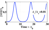
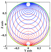
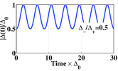
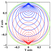
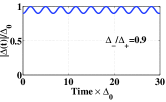
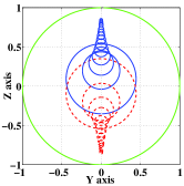
FIG. 1.: Coherent BCS dynamics on the Bloch sphere (16). Trajectories of individual Cooper pair states for the soliton train solutions (Eq. (26) and insets) oscillating in the limits $\Delta_{-}\leq\Delta(t)\leq\Delta_{+}$ are shown. Note that each state completes a full $2\pi$ Rabi cycle per soliton. The red and blue curves correspond to the energies $\epsilon_{{\bf p}}$ above and below the Fermi level.

At $T=0$, in the case of a constant density of states, $\gamma$ is equal to the equilibrium BCS gap $\Delta_{0}$, while $\omega$ vanishes due to particle-hole symmetry. Thus, remarkably, the modulus $|\Delta(t)|$ in this case peaks exactly at $\Delta_{0}$.

To illustrate the collective dynamics in the soliton solution, we plot the trajectories $u_{{\bf p}}(t)$, $v_{{\bf p}}(t)$ on the Bloch sphere $r_{1}^{2}+r_{2}^{2}+r_{3}^{2}=1$ using the parameterization

$$r_{1}+ir_{2}=2u_{{\bf p}}v^{\ast}_{{\bf p}};\quad r_{3}=|u_{{\bf p}}|^{2}-|v_{{\bf p}}|^{2}$$ (16)

(Fig. 1, left). Here, as well as in the soliton train solutions discussed below (Eq. (26)), each state $(u_{{\bf p}},v_{{\bf p}})$ completes a full Rabi cycle per soliton. The trajectories, which are small loops for the pairs with large energies $\epsilon_{{\bf p}}$, turn into a big circle as $\epsilon_{{\bf p}}$ tends to the Fermi level.

To gain further insight, we reformulate the Bogoliubov approach, following Anderson [23], in terms of pseudospins associated with individual Cooper pair states. ‘Pauli spin’ operators $\sigma^{\pm}_{{\bf p}}\equiv\frac{1}{2}(\sigma^{x}_{{\bf p}}\pm i\sigma^{y}_{{\bf p}})$ can be assigned to each pair of fermions with opposite momenta as follows

$$\sigma^{+}_{{\bf p}}=a^{+}_{{\bf p}\uparrow}a^{+}_{-{\bf p}\downarrow}\,,\quad\sigma^{-}_{{\bf p}}=a_{-{\bf p}\downarrow}a_{{\bf p}\uparrow}$$ (17)

The identity $\sigma^{z}_{{\bf p}}\equiv[\sigma^{+}_{{\bf p}},\sigma^{-}_{{\bf p}}]=a^{+}_{{\bf p}\uparrow}a_{{\bf p}\uparrow}-a_{-{\bf p}\downarrow}a^{+}_{-{\bf p}\downarrow}$ allows to map the problem (2) onto an interacting spin problem

$${\cal H}={\sum_{{\bf p}}}^{\prime}\epsilon_{{\bf p}}\sigma^{z}_{{\bf p}}-2\lambda{\sum_{{\bf p},{\bf q}}}^{\prime}\sigma^{+}_{{\bf p}}\sigma^{-}_{{\bf q}}$$ (18)

where ${\sum}^{\prime}_{{\bf p}}$ means a sum over the pairs of states $({\bf p},-{\bf p})$. Since all the spins interact with each other equally, the mean field theory here is exact, just like for the BCS problem. The mean field hamiltonian for each spin is

$${\cal H}_{{\bf p}}={\bf b}_{{\bf p}}\cdot{\bf\sigma_{{\bf p}}},\quad{\bf b}_{{\bf p}}=\left(-\Delta^{\prime},-\Delta^{\prime\prime},\epsilon_{{\bf p}}\right)$$ (19)

Here the $z$ component of the effective field ${\bf b}_{{\bf p}}$, given by the single particle energy, is spin-specific, while the transverse components, the same for all of the spins, satisfy

$$\Delta\equiv\Delta^{\prime}+i\Delta^{\prime\prime}=\lambda\sum_{{\bf q}}\langle\sigma^{+}_{{\bf q}}\rangle$$ (20)

which is analogous to the BCS gap relation. In the ground state each spin is aligned with ${\bf b}_{{\bf p}}$, and the spins form a texture near the Fermi surface [23], with spin rotation described by the Bogoliubov angle.

The dynamical problem of interest can be cast in the form of Bloch equations for the spins,

$$\dot{\sigma}_{{\bf p}}=i[{\cal H}_{{\bf p}},\sigma_{{\bf p}}]=2{\bf b}_{{\bf p}}\times{\bf\sigma}_{{\bf p}}$$ (21)

with the field ${\bf b}_{{\bf p}}$ defined selfconsistently by (19),(20). Anderson [23] used Eq. (21), linearized about the texture ground state, to study collective excitations of a superconductor (see also [24]). Linearized about the unpaired state, Eq. (21) yields an instability identical to (6), (7).

The Bloch dynamics is suitable for simulation (Fig. 2), since Eq. (21) is linear in spin operators and can be replaced by an equation for the expectation values (16). Typical $\Delta(t)$, observed in the presence of thermal noise, is an orderly sequence of the $\cosh{}$ solitons (Fig. 2, top), indicating robustness of soliton solution (cf. Ref.[25]).

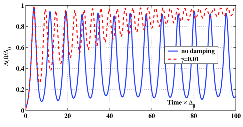
FIG. 2.: Bloch dynamics $\dot{\bf r}_{{\bf p}}=2{\bf b}_{{\bf p}}^{\rm eff}\times{\bf r}_{{\bf p}}$ for $10^{3}$ spins with a constant density of states, with ${\bf b}_{{\bf p}}^{\rm eff}$ defined by (19),(22). Initial conditions $r_{3,{\bf p}}=\tanh(\textstyle{\frac{1}{2}}\beta\epsilon_{{\bf p}})$, $(r_{1}\!+\!ir_{2})_{{\bf p}}=e^{i\phi_{{\bf p}}}(1-r_{3}^{2})^{1/2}$, with $\beta^{-1}\equiv T=0.1\Delta_{0}$ and random uncorrelated $0<\phi_{{\bf p}}<2\pi$ were used to simulate thermal noise.

The effect of damping can be studied by replacing

$${\bf b}_{{\bf p}}\to{\bf b}_{{\bf p}}^{\rm eff}={\bf b}_{{\bf p}}-\gamma{\bf b}_{{\bf p}}\times{\bf r}_{{\bf p}}$$ (22)

with a dimensionless damping constant, $\gamma\sim 1/(\Delta_{0}\tau_{\epsilon})$. This destroys integrability and prompts relaxation to BCS equilibrium (Fig. 2, bottom).

In our nonlinear dynamical problem, we have to solve the Bloch equations (21) together with the selfconsistency relation (20). As above, we assume the pairing amplitude time dependence of the form $\Delta(t)=e^{-i\omega t}\Omega(t)$, where $\Omega(t)$ is real and $\omega$ is a constant frequency shift to be fixed by the relation (20). In the Larmor frame rotating with the frequency $\omega$, Eq. (21), written for the spins average polarization $r_{i}=\langle\sigma^{i}_{{\bf p}}\rangle$ components, reads

$$\dot{r}_{1}=-\xi_{{\bf p}}r_{2},\quad\dot{r}_{2}=\xi_{{\bf p}}r_{1}+2\Omega r_{3},\quad\dot{r}_{3}=-2\Omega r_{2}$$ (23)

with $\xi_{{\bf p}}=2\epsilon_{{\bf p}}-\omega$, as before. An exact solution can be obtained from the ansatz

$$r_{1}=A\Omega,\quad r_{2}=B\dot{\Omega},\quad r_{3}=C\Omega^{2}-D$$ (24)

The first and the third equation (23) are satisfied by (24) provided $A=-\xi_{{\bf p}}B$ and $B=-C$, while the second equation (23) is consistent with the normalization condition $r_{1}^{2}+r_{2}^{2}+r_{3}^{2}=1$, and thus yields

$$C^{2}\xi_{{\bf p}}^{2}\Omega^{2}+C^{2}\dot{\Omega}^{2}+(C\Omega^{2}-D)^{2}=1$$ (25)

Eq. (25) will take the same form for all the spins,

$$\dot{\Omega}^{2}+(\Omega^{2}-\Delta^{2}_{-})(\Omega^{2}-\Delta^{2}_{+})=0,\quad\Delta_{-}\leq\Delta_{+}$$ (26)

provided that the constants $D$, $C$ are chosen as

$$(D^{2}-1)/C^{2}=\Delta^{2}_{-}\Delta^{2}_{+},\quad 2D/C=\xi_{{\bf p}}^{2}+\Delta^{2}_{-}+\Delta^{2}_{+}$$ (27)

with the sign factor ${\rm sgn}\,\epsilon_{{\bf p}}$. Eq. (26) defines an elliptic function $\Omega(t)$ oscillating periodically between $\Delta_{-}$ and $\Delta_{+}$. At $\Delta_{-}\ll\Delta_{+}$, the solution is a train of weakly overlapping solitons (14) with $\Delta_{+}=\gamma$ (Fig. 1, left).

The real part of the selfconsistency relation (20),

$$1=\lambda\sum_{{\bf p}}\frac{\xi_{{\bf p}}{\rm sgn}\,\epsilon_{{\bf p}}}{\left((\xi_{{\bf p}}^{2}+\Delta^{2}_{-}+\Delta^{2}_{+})^{2}-4\Delta^{2}_{-}\Delta^{2}_{+}\right)^{1/2}}$$ (28)

fixes one of the constants $\Delta_{\pm}$, the other one being a free parameter that controls the inter-soliton time separation. With the ratio $\Delta_{-}/\Delta_{+}$ varying from $0$ to $1$, the soliton frequency increases, and the weakly overlapping solitons (14) gradually become overlapping more strongly, turning into weak harmonic oscillations (Fig. 1).

We note that the weak oscillation limit has been investigated by Volkov and Kogan [24] with the help of linearized Gorkov equation, and earlier by Anderson [23], who used pseudospin representation. The nonexponential decay of the lianearized oscillations [18, 24] was interpreted as collisionless damping, related to strong mixing of the oscillations of $\Delta$ with the states of two excited quasiparticles slightly above the superconducting gap.

The imaginary part of Eq. (20) fixes the value of the frequency shift $\omega$ (we recall that $\omega\neq 0$ in the presence of charge asymmetry). At $\Delta_{-}\ll\Delta_{+}$, Eq. (28) turns into Eq. (7) which, as we found above, defines the amplitude of a single soliton. In the opposite limit, $\Delta_{-}\to\Delta_{+}$, Eq. (28) coincides with the BCS gap equation.

There is an interesting relation between our problem and the self-induced transparency phenomenon [26]. In the latter, an optical pulse interacting with an ensemble of atoms can dissipate its energy by inducing resonant Rabi transitions in the atoms. However, when the pulse duration is tuned so that the atoms complete a full Rabi $2\pi$ cycle as the pulse goes by, the pulse sustains itself and propagates without dissipation. The Bloch equations describing this phenomenon bear striking similarity to our Eqs. (21), while the atoms’ polarization is employed [26] to provide feedback on the pulse instead of our BCS selfconsistency relation.

Before concluding, we note that the dynamics at finite temperature, in the regime described by Eq. (1), remains an open problem. In particular, we can not rule out the possibility of chaotic behavior. At $T=0$ the problem has a relatively simple solution, periodic in time, because in this case the quasiparticles with low energies are strongly coupled to the oscillations of $\Delta$. In contrast, in the case $T\tau_{\Delta}\gg 1$ there are two groups of quasiparticles: those with energies $\epsilon_{{\bf p}}\sim\tau_{\Delta}^{-1}$, which fully participate in the oscillations, as above, and the quasiparticles with $\tau_{\Delta}^{-1}\ll\epsilon_{{\bf p}}\ll T$, coupled to $\Delta(t)$ much weaker and playing the role of a thermal bath, thereby providing dissipation.

In summary, this work provides an exact solution for the BCS pairing formation problem. In the nonadiabatic regime, the dynamics is dissipationless and thus nonlinear. Soliton train solutions are obtained analytically and demonstrated to be generic and robust by a simulation.

REFERENCES

- [1] B. DeMarco, et al., Phys. Rev. Lett. 82, 4208 (1999); Science 285, 1703 (1999); Phys. Rev. Lett. 86, 5409 (2001); Phys. Rev. Lett. 88, 040405 (2002); A. G. Truscott et al., Science 291, 2570 (2001); T. Loftus et al., Phys. Rev. Lett. 88, 173201 (2002); K. M. O’Hara, et al., Science 298, 2179 (2002); Phys. Rev. A 66, 041401 (2002)
- [2] H. T. C. Stoof, M. Houbiers, C. A. Sackett, and R. G. Hulet, Phys. Rev. Lett. 76, 10 (1996)
- [3] Tin-Lun Ho and S. Yip, Phys. Rev. Lett. 82, 247 (1999)
- [4] J. L. Bohn, Phys. Rev. A61, 053409 (2000)
- [5] M. Holland, S. J. J. M. F. Kokkelmans, M. L. Chiofalo, and R. Walser, Phys. Rev. Lett. 87, 120406 (2001)
- [6] S. J. J. M. F. Kokkelmans, J. N. Milstein, M. L. Chiofalo, R. Walser, and M. J. Holland, Phys. Rev. A65, 053617 (2002)
- [7] J. N. Milstein, S. J. J. M. F. Kokkelmans, and M. J. Holland, Phys. Rev. A66, 043604 (2002)
- [8] Y. Ohashi, and A. Griffin, Phys. Rev. Lett. 89, 130402 (2002); Phys. Rev. A67, 033603 (2003); Phys. Rev. A67, 063612 (2003)
- [9] J. Stajic, J. N. Milstein, Q. Chen, M. L. Chiofalo, M. J. Holland, and K. Levin, cond-mat/0309329
- [10] H. Heiselberg, C. J. Pethick, H. Smith, and L. Viverit, Phys. Rev. Lett. 85, 2418 (2000)
- [11] M. A. Baranov, M. S. Mar enko, V. S. Rychkov, and G. V. Shlyapnikov, Phys. Rev. A 66, 013606 (2002)
- [12] H. Heiselberg and B. Mottelson, Phys. Rev. Lett. 88, 190401 (2002)
- [13] C. P. Search, H. Pu, W. Zhang, B. P. Anderson, and P. Meystre, Phys. Rev. A 65, 063616 (2002)
- [14] J. Carlson, S.-Y. Chang, V. R. Pandharipande, and K. E. Schmidt, Phys. Rev. Lett. 91, 050401 (2003)
- [15] H. Heiselberg, Phys. Rev. A 68, 053616 (2003)
- [16] M. Houbiers and H. T. C. Stoof, Phys. Rev. A59, 1556 (1999)
- [17] M. Tinkham, Introduction to Superconductivity, (McGraw-Hill, 1996)
- [18] A. Schmid, Phys. Kond. Mat. 5, 302 (1966)
- [19] E. Abrahams and T. Tsuneto, Phys. Rev. 152, 416 (1966)
- [20] L. P. Gor’kov, G. M. Eliashberg, Zh. Eksp. Teor. Fiz. 54, 612 (1968) [Sov. Phys. JETP 27, 328 (1968)]
- [21] A. G. Aronov and V. L. Gurevich, Sov. Phys. Solid State, 16, 1722, (1974); Sov. Phys. JETP, 38, 550, (1974);
- [22] A. I. Larkin, Yu. N. Ovchinnikov, Sov. Phys. JETP, 46, 155, (1977)
- [23] P. W. Anderson, Phys. Rev. 112, 1900 (1958)
- [24] A. F. Volkov and Sh. M. Kogan, Sov. Phys. JETP, 38, 1018 (1974);
- [25] Yu. M. Gal’perin, V. I. Kozub, and B. Z. Spivak, Sov. Phys. JETP, 54, 1126 (1981)
- [26] S. L. McCall and E. L. Hahn, Phys. Rev. Lett. 18, 908 (1967); Phys. Rev. 183, 457 (1968)