Geometry and the Hidden Order of Luttinger Liquids: the Universality of Squeezed Space.

Abstract

We present the case that Luttinger liquids are characterized by a form of hidden order which is similar, but distinct in some crucial regards, to the hidden order characterizing spin-1 Heisenberg chains. We construct a string correlator for the Luttinger liquid which is similar to the string correlator constructed by den Nijs and Rommelse for the spin chain. We re-analyze the spin one chain, introducing a precise formulation of the geometrical principle behind the so-called ‘squeezed space’ construction, to demonstrate that the physics at long wavelength can be reformulated in terms of a $Z_{2}$ gauge theory. Peculiarly, the normal spin chain lives at infinite gauge coupling where it is characterized by deconfinement. We identify the microscopic conditions required for confinement thereby identifying a novel phase of the spin-chain. We demonstrate that the Luttinger liquid can be approached in the same general framework. The difference from the spin chain is that the gauge sector is critical in the sense that the Luttinger liquid is at the phase boundary where the $Z_{2}$ local symmetry emerges. In addition, the ‘matter’ (spin) sector is also critical. We evaluate the string correlator analytically for the strongly coupled Hubbard model and further we demonstrate that the squeezed space structure is still present even in the non-interacting fermion gas. This adds new insights to the meaning of bosonization. These structures are hard-wired in the mathematical structure of bosonization and this becomes obvious by considering string correlators. Numerical results are presented for the string correlator using a non-abelian version of the density matrix renormalization group algorithm, confirming in detail the expectations following from the theory. We conclude with some observations regarding the generalization of bosonization to higher dimensions.

I Introduction

The Luttinger liquid, the metallic state of one dimensional electron matter, is an old subject which is believed to be fully understood. In the 1970’s the bosonization theory was developed which has a similar status as the Fermi-liquid theory, making possible to compute long wavelength properties in detail with only a small number of input parametersVoitSchulz ; Stone . In the present era, the theory is taken for granted, and it has found many applications, most recently in the context of nanophysicsDekker . Here we will attempt to persuade the reader that there is still something to be learned about the fundamentals of the Luttinger liquid.

In first instance, it is intended as a clarification of some features of the Luttinger liquid which appear as rather mysterious in the textbook treatments. We make the case that a physical conception is hidden in the mathematics of the standard treatise. This physical conception might alternatively be called ‘hidden order’, ‘critical gauge deconfinement’ or ‘fluctuating bipartite geometry’. It all refers to the same entity, viewed from different angles. This connection was first explored in our previous letterLetter , here we expand on these ideas to yield some practical consequences: (a) we identify symmetry principles allowing a sharp distinction between Luttinger liquids and for instance the bosonic liquids found in spin-1 chainsNijs (the ‘no-confinement’ principle, sections II, III), (b) we identify a new competitor of the Luttinger liquid (the manifestly gauge invariant superconductor, section III, a close sibling of the superfluid $t-J$ model of Batista and OrtizBatista ), and (c) these insights go hand in hand with special ‘string’ (or ‘topological’) correlation functions which makes possible unprecedented precision tests of the analytical theory by computer simulations, offering also advantages for the numerical determination of exponents (section VI).

This pursuit was born out from a state of confusion we found ourselves in some time ago, caused by a view on the Luttinger liquid from an unusual angle. Our interest was primarily in what is now called ‘stripe fractionalization’Zaanenphilmag ; Nussinov ; Sachdev0 ; Sachdev1 . Stripes refer to textures found in doped Mott-insulators in higher dimensions. These can be alternatively called ‘charged domain walls’Zaanen89 : the excess charges condense on $d-1$ dimensional manifolds, being domain walls in the colinear antiferromagnet found in the Mott-insulating domains separating the stripes. Evidence accumulated that such a stripe phase might be in close competition with the high-$Tc$ superconducting state of the cupratesZaanenphilmag ; Kivelson and this triggered a theoretical effort aimed at an understanding of stripe quantum liquids. The idea emerged that in principle a superconductor could exist characterized by quantum-delocalized stripes which are however still forming intact domain walls in the spin system. Using very similar arguments as found in sections II and III of this paper, it can then be argued that several new phases of matter exist governed by Ising gauge theory. This is not the subject of this paper and we refer the interested reader to the literatureZaanenphilmag ; Nussinov ; Sachdev0 ; Sachdev1 . However, we realized early on that these ideas do have an intriguing relationship with one dimensional physics.

Specifically, we were intrigued by two results which, although well known, do not seamlessly fit into the Luttinger liquid mainstream: (a) the hidden order in Haldane spin chains as discovered by den Nijs and RommelseNijs , (b) the squeezed space construction as deduced by WoynarovichWoyn , Ogata and Shibaogashi from the $U\rightarrow\infty$ Bethe Ansatz solution of the Hubbard model. As we will discuss in much more detail, after some further thought one discovers that both refer to precisely the same underlying structure. This structure can be viewed from different sides. Ogata and Shibaogashi emphasize the geometrical side: it can be literally viewed as a dynamically generated ‘fluctuating geometry’, although one of a very simple kind. Den Nijs and Rommelse approached it using the language of orderNijs : a correlation function can be devised approaching a constant value at infinity, signaling symmetry breaking. The analogy with stripe fractionalization makes it clear that it can also be characterized as a deconfinement phenomenon in the language of gauge theory.

Whatever way one calls it, this refers to a highly organized, dynamically generated entity. The reason we got confused is that there is no mention whatsoever in the core literature of the Luttinger liquid of how these squeezed spaces etcetera fit in the standard bosonization lore. To shed some light on these matters we found inspiration in the combined insights of den Nijs-Rommelse and Ogata-Shiba and we constructed a den Nijs type ‘string’ correlator but now aimed at the detection of the squeezed space of Ogata and Shiba. This is the principal device that we use, and it has the form,

$$O_{str}(|i-j|)=\langle\;\vec{S}_{i}\;\left[\Pi_{l=i}^{j}(-1)^{n_{i}}\right]\;\vec{S}_{j}\;\rangle\;,$$ (1)

where $\vec{S}_{i}$ is the spin-operator on site $i$ while $n_{l}$ measures the charge density. By studying the behavior of this correlator one can unambiguously establish the presence of squeezed-space like structures. We spend roughly the first half of this paper explaining how this works and what it all means. In section II we start with a short review of the den Nijs-Rommelse work on the $S=1$ ‘Haldane’Haldane spin chains. This is an ideal setting to develop the conceptual framework. We subsequently reformulate the spin chain ‘string’ correlator in a geometrical setting which makes the relationship with the Woynarovich-Ogata-Shiba squeezed space manifest. We finish this section with the argument why it is Ising gauge theory in disguise. This is helpful, because the gauge theory sheds light on the limitations of the squeezed space: we present a recipe of how to destroy the squeezed space structure of the spin chain.

In section III we revisit Woynarovich-Ogata-Shiba. The string correlator Eq. (1) is formulated and subsequently investigated in the large $U$ limit. This analysis shows that the Luttinger liquid (at least for large $U$) can be viewed as the critical version of the Haldane spin chain. It resides at the phase transition where the gauge invariance emerges, while the matter fields are critical as well. In this section we also argue why the squeezed space of the electron liquid cannot be destroyed. This turns out to be an unexpected consequence of Fermi-Dirac statistics.

In the remaining two sections the string correlator is used to interrogate the Luttinger liquid regarding squeezed space away from the strong coupling limit. In section IV we demonstrate in a few lines a most surprising result: squeezed space exists even in the non-interacting spinful fermion gas! This confirms in a dramatic way that squeezed space is deeply rooted in fermion statistics; it is a complexity price one has to pay when one wants to represent fermion dynamics in one dimension in terms of bosonic variables.

In section V we turn to bosonization. Viewing the bosonization formalism from the perspective developed in the previous sections it becomes clear that the squeezed space structure is automatically wired into the structure of the theory. In this regard, the structure of bosonization closely parallels the exact derivations presented in section III. In section VI we present numerical density matrix renormalization group (DMRG) calculations for the string correlators starting from the Hubbard model at arbitrary fillings and interaction strength, employing a non-abelian algorithm. These results confirm in a great detail the expectations build up in the previous sections: the strongly interacting limit and the non-interacting gas are smoothly connected and in the scaling limit the string correlator Eq. (1) isolates the spin only dynamics regardless the microscopic conditions. This has also practical consequences; we deliver the proof of principle that the non-universal exponents associated with the logarithmic corrections showing up in the spin-correlations can be addressed away from half-filling. From the combination of bosonization and the exact results for strong coupling suggest that the two point spin correlator can always be written in the scaling limit as the product of Eq(1) and a charge-like string correlator,

$$\langle\vec{S}(x)\vec{S}(0)\rangle\;\sim\;D_{nn}(x)\;O_{str}(x)\;,$$ (2)

where the ‘charge’ string operator is defined as,

$$D_{nn}(|i-j|)\;\equiv\;\langle\;n_{s}(i)\;\left[\Pi_{l=i}^{j}(-1)^{n_{s}(l)}\right]\;n_{s}(j)\rangle\,$$ (3)

where $n_{s}(i)$ is 1 for a singly occupied site and 0 otherwise. We confirm numerically that except for a non-universal amplitude the relation Eq. (2) seems always satisfied at long distances.

The conclusion to this paper addresses the broader perspective including the relation to stripe fractionalization in 2+1 dimensions.

II Geometry, gauge theory and Haldane spin chains.

The ‘Haldane’Haldane $S=1$ Heisenberg spin chains are an ideal stage to introduce the notions of ‘hidden order’, squeezed space, and the relation with Ising gauge theory. These systems are purely bosonic, i.e. dualization is not required for the identification of the bosonic fields, and the powers of bosonic field theory can be utilized with great success to enumerate the physics completely. We refer in particular to the mapping by den Nijs and RommelseNijs on surface statistical physics. We are under the impression that this way of thinking is not widely disseminated and we start out reviewing some highlights. In the surface language, the meaning of ‘hidden-order’ becomes particularly simple (section II.1). We subsequently use these simple insights to reformulate this hidden order in the geometrical language, the ‘squeezed space’ (section II.2). The next benefit of the Haldane chain is that the identification of squeezed space geometry with Ising gauge theory is literal (section II.3). This sets the conceptual framework within which we view the Luttinger liquid.

II.1 Haldane spin chains: a short review

Let us first review some established wisdoms concerning the Haldane spin chains. The relevant model is a standard Heisenberg model for $S=1$ extended by biquadratic exchange interactions and single-ion anisotropy,

$$H=\sum_{<ij>}\vec{S}_{i}\cdot\vec{S}_{j}+\alpha\sum_{<ij>}(\vec{S}_{i}\cdot\vec{S}_{j})^{2}+D\sum_{i}(S^{z}_{i})^{2}\;.$$ (4)

In the proximity of the Heisenberg point ($\alpha=D=0$) the ground state is a singlet, separated by a finite energy gap from propagating triplet excitations. It was originally believed that the long distance physics was described by an $O(3)$ non-linear sigma modelHaldane , suggesting that the ground state is featureless singlet. However, Affleck et alAKLT discovered that for $\alpha=1/3,D=0$ the exact ground state wavefunction can be deduced, having a particularly simple form. This ‘AKLT’ wavefunction can be parametrized as follows. Split the $S=1$ microscopic singlets into two Schwinger bosons $|S=1,M_{s}\rangle\sim b^{\dagger}_{i1,\alpha}b^{\dagger}_{i2,\alpha}$. The individual Schwinger bosons carry $S=1/2$ and the wavefunction is constructed by pairing, say, the ‘1’ boson with a ‘1’ boson on the left neighboring site forming a singlet of valence bond, and the same with the ’2’ boson with its counterpart on the right neighbor,

$$\begin{array}[]{rcl}|\Psi\rangle_{AKLT}&=&2^{-N/2}\left[\cdots(b^{\dagger}_{i-1;1\uparrow}b^{\dagger}_{i;1\downarrow}-b^{\dagger}_{i-1;1\downarrow}b^{\dagger}_{i;1\uparrow})\;(b^{\dagger}_{i;2\uparrow}b^{\dagger}_{i+1;2\downarrow}-b^{\dagger}_{i;2\downarrow}b^{\dagger}_{i+1;2\uparrow})\right.\\ &&\left.\times(b^{\dagger}_{i+1;1\uparrow}b^{\dagger}_{i+2;1\downarrow}-b^{\dagger}_{i+1;1\downarrow}b^{\dagger}_{i+2;1\uparrow})\cdots\right]|\textrm{vac}\rangle\end{array}$$ (5)

This wave function clearly has to do with a translation symmetry breaking involving nearest-neighbor singlet pairs, although in terms of spin-degrees of freedom which are different from the elementary spins. It has become a habit to call it ‘valence bond solid order’, i.e. to link it exclusively to the tendency in the spin system to form spin $1/2$ singlet pairs. Den Nijs and RommelseNijs added a deep understanding of the physics of these bosonic spin chains by introducing the mapping on surface statistical physics. Although the AKLT wave function is a correct prototype for the ground state of the Heisenberg chain, it is not helpful with regard to what else can happen. On the other hand, by employing the formidable powers of surface statistical physics there are no secrets and it yields a natural view on the physics of the spin-chains. A highlight is their demonstration that this vacuum can be understood by a a non-local (‘topological’) order parameter structure in terms of the real $S=1$ spin degrees of freedom. The measure of order is the asymptotic constancy of a correlation function. The conventional two-point spin correlator in the Haldane chain decays exponentially for large $|i-j|$,

$$\langle S^{z}_{i}\;S^{z}_{j}\rangle\sim e^{-|i-j|/\xi}$$ (6)

However, considering the following non-local spin correlator (or ’string’ correlator),

$$\langle S^{z}_{i}\;\left[\Pi_{l=i}^{j}(-1)^{S^{z}_{l}}\right]\;S^{z}_{j}\rangle\sim\text{constant}$$ (7)

signaling a form of long range order which only becomes visible when probed through the non-local correlator Eq. (7). For this reason it was called ‘hidden order’. A main purpose of this section will be to introduce a more precise definition of this order.

Den Nijs and RommelseNijs deduced the string correlator using the insights following from the path-integral mapping onto surface statistical physics. A first, crucial observation is that the natural basis for the spin chain is not in terms of generalized coherent states, but instead simply in terms of the microscopic $M_{s}=0,\pm 1$ states of individual spins. Marshall signs are absent and these states can be parametrized in terms of flavored bosons $b^{\dagger}_{0},b^{\dagger}_{\pm 1}$ subjected to a local constraint $\sum_{\alpha}b^{\dagger}_{\alpha}b_{\alpha}=1$. The spin operators become,

$$S^{z}_{i} = n_{i,1}-n_{i,-1}$$

$$S^{+}_{i} = \sqrt{2}\left(b^{\dagger}_{i,1}b_{i,0}+b^{\dagger}_{i,0}b_{i,-1}\right)$$

$$S^{-}_{i} = \sqrt{2}\left(b^{\dagger}_{i,0}b_{i,1}+b^{\dagger}_{i,-1}b_{i,0}\right)$$ (8)

A second crucial observation is that because of the constraint the problem is isomorphic to that of a (directed) quantum string living on a square lattice. This is somewhat implicit in the original formulation by den Nijs and Rommelse, but used to great effect by Eskes et al.Eskes . The mapping is elementary. A lattice string corresponds with a connected trajectory of ‘particles’ living on a lattice and this string can in turn be parametrized by a center of mass coordinate and the set of links connecting all particles. Consider only ‘forward moving’ links (the string is directed) and identify a nearest-neighbor link with a $M_{s}=0$ bond, and an ‘upward’ and ‘downward’ next-nearest-neighbor link (‘kinks’) with $M_{s}=1$ and $M_{s}=-1$ states of the spin on a site of the Haldane chain, respectively. It is easy to convince oneself that every state in the Hilbert space of the spin chain corresponds with a particular string configuration. The XY terms are responsible for the creation of kink-antikink pairs and the propagation of individual kinks along the string, while Ising terms govern the interactions between the kinks. In the path integral formulation, quantum strings spread out into world-sheets and the world-sheet of the lattice string corresponds with a surface statistical physics which is completely understood: the restricted solid-on-solid (RSOS) surface.

Figure 1: Mapping of the spin chain on a directed quantum string living on a lattice Eskes . The $M_{s}=0,\pm 1$ states of the spin chain are equivalent to horizontal-, and upward/downward diagonal links tracing out the trajectory of the string on the lattice. The $XY$ terms in the spin Hamiltonian correspond with the kinetic energy of the string problem causing both the creation of kink-antikink pairs (the $\pm 1$ bonds) and the coherent propagation of individual kinks. At the Heisenberg- and AKLT points hidden order is present. Although kinks are proliferated their direction is ordered: every up kink is followed by a down kink (a). In the string representation this just means that the string pins to the links of the lattice. In the rough ($XY$) phase kinks have proliferated while their direction is disordered as well (b).

The topological order of the Haldane spin chain translates into a simple form of order in the surface language: the disordered flat phase. The $+1$ and $-1$ kinks on the time slice turn into up and down steps on the world-sheet in space time, see Fig. (1). In the disordered flat phase these steps have proliferated (kinks occur at finite density while they are delocalized) but on this surface every ‘up’ step is followed by a down step and the surface as a whole is still flat, pinned to the lattice. In the string language the order is therefore manifest, but it becomes elusive when translated back to the spin system. It implies that the ground state of the spin chain is a coherent superposition of a special class of states. These are composed of indeterminate mix of $0,\pm 1$ states. Take the $0$’s as a reference vacuum and view the $M_{s}=\pm 1$ states as particles carrying an in internal ‘flavor’ $\pm 1$. These particles are delocalized. However, every $+1$ particle is followed by a $-1$ particle, modulo local violations (virtual excitations) which can be integrated out perturbatively (fig. 1). The hidden order is thereby nothing else than the staggered order of the $\pm 1$ flavors of the ‘spin particles’. This order is not seen by the spin-1 operators because these also pick up the positional disorder of the $\pm 1$ ‘particles’.

II.2 Squeezed space: sublattice parity as a gauge freedom.

String correlators of the kind Eq. (7) have the purpose of ‘dividing out’ the positional disorder with the effect that the order of the ‘internal’ $\pm 1$ flavors becomes observable. In order to see the similarity with the phenomena occurring in the Luttinger liquid we need a more precise description of how this ‘division’ is accomplished than that found in the original literature. It amounts to a geometrical mapping of a simple kind. The string correlator can be written in terms of the bosons as,

$$\begin{array}[]{rcl}\langle S^{z}_{i}\left[\Pi_{l=i}^{j}(-1)^{S^{z}_{l}}\right]S^{z}_{j}\rangle&\equiv&\left\langle(n_{i,1}-n_{i,-1})\right.\\ &&\times\;\Pi_{l=i}^{j}(-1)^{1-n_{l,0}}\\ &&\times\;\left.(n_{j,1}-n_{j,-1})\right\rangle\end{array}$$ (9)

Why is this tending to a constant while the two-point spin correlator is decaying exponentially? From the discussion in section II.1 it follows that modulo local fluctuations the ground state wave function has the form,

$$|\Psi\rangle=\sum\;a(x_{1},x_{2},...,x_{2i},x_{2i+1},...)\;|x_{1}(1),x_{2}(-1),...,x_{2i}(-1),x_{2i+1}(1),...\rangle$$ (10)

where the $x_{i}$’s refer to the positions of the $\pm 1$ particles on the chain, and the amplitudes $a$ are independent from the ‘internal’ ($\pm 1$) degrees of freedom; these ‘internal’ Ising spins show the antiferromagnetic order. In order to construct a two point correlator capable of probing this ‘internal’ order it is necessary to redefine the space in which the internal degrees of freedom live. Start out with the full spin chain and for each configuration, whenever a site occupied by a 0-particle is found remove this site and shift, say, all right neighbors to the left, see fig. (2). This new space is called ‘squeezed space’ and the effect of the map from ‘full’ to squeezed space is such that every configuration appearing in Eq. (10) maps on the same antiferromagnetic order as realized on the squeezed chain.

Figure 2: The geometrical mapping from ‘full’ (a) to ‘squeezed’ space (b). Given that some antiferromagnet lives in squeezed space, all that matters is the fate of the sublattice parity $p$. When sites are reinserted, the sublattice parity of the system in squeezed space flips every time a hole is passed when viewed in full space. These sublattice parity flips hide the order present in squeezed space.

Obviously, if it would be possible to probe squeezed space directly, the hidden order would be measurable using conventional two point correlators. The string correlator achieves just this purpose. All that matters is that the order in squeezed space is a staggered (antiferromagnetic) order. For such order one needs a bipartite geometry: it should be possible to divide the lattice into $A$ and $B$ sublattices such that every site on the $A$ sublattice is neighbored by $B$ sublattice sites and vice versa. In one dimension any space is bipartite (even the continuum). This subdivision can be done in two ways: $\cdots A-B-A-B\cdots$ or $\cdots B-A-B-A\cdots$, corresponding with the $Z_{2}$ valued quantity we call sublattice parity. For a normal lattice the choice of sublattice parity is arbitrary, it is a ‘pure gauge’. However, in the mapping of squeezed to full space it becomes ‘alive’, actually in a way which is in close correspondence to the workings of a dynamical $Z_{2}$ gauge field as will become clear later. Consider what happens when squeezed space is unsqueezed (Fig.2). When a ‘0’ particle including its site is reinserted, the ‘flavor’ site, say, on its right side is shifted one lattice constant to the right. The effect is that relative to the reference sublattice parity of squeezed space the sublattice parity in unsqueezed space changes sign every time a ‘0’ particle is passed. The effect is that flips in the sublattice appear to be ‘bound’ to the $0$ particles viewing matters in full space. In order to interrogate the ‘flavor’ order in squeezed space one has to remove these sublattice parity flips. This can be achieved by multiplying the spin with a minus one every time a 0 particle is encountered: $(-1)\times(-1)^{l+1}=(-1)^{l}$. The den Nijs string operator is constructed to precisely achieve this purpose,

$$\begin{array}[]{l}\langle(n_{i,1}-n_{i,-1})\left[\Pi_{l=i}^{j}(-1)^{1-n_{l,0}}\right](n_{j,1}-n_{j,-1})\rangle\\ \quad\equiv\langle(-1)^{i}(n_{i,1}-n_{i,-1})\left[\Pi_{l=i}^{j}(-1)^{n_{l,0}}\right](-1)^{j}(n_{j,1}-n_{j,-1})\rangle\end{array}$$ (11)

Hence the string correlator measures the spin order in squeezed space by removing the sublattice parity flips. The positional disorder of the particles is equivalent to motions of the sublattice parity flips, scrambling the order living in squeezed space, and these are removed by the string operators.

Figure 3: Same as Fig. (2) but now for the case that an Ising long range order is present in squeezed space, corresponding with the hidden order of the $S=1$ Heisenberg spin chain. From such pictures one can directly deduce the workings of string operators by just focusing on the spins. However, matters are equally meaningful in the absence of long range order in squeeze space, and the formulation terms of a geometrical mapping involving sublattice parity is more general.

The above argument emphasizes the geometrical nature of the mechanism hiding the order. It might at this point appear as a detour because one arrives at the same conclusion by just focusing on the ‘flavor’ orientations, see Fig. (3). However, as will become clear in later sections, the construction is still applicable even when the spin system in squeezed space is disordered. Hence, it is more general and rigorous to invoke the geometrical sublattice parity as a separate degree of freedom in addition to the degrees of freedom populating squeezed space.

II.3 Squeezed spaces and Ising gauge theory.

At first sight, it might appear that sublattice parity is not quite like a normal dynamical degree of freedom. However, it is easily seen that it is nothing else than an uncommon ultraviolet regularization of $Z_{2}$ gauge fields. From the above discussion it is clear that the ‘flavor’ degrees of freedom of the $\pm 1$ particles can be regarded as independent from their positions in unsqueezed space. These flavors are $Z_{2}$ valued and can be measured by,

$$\tau^{z}_{i}=(1-b^{\dagger}_{i,0}b_{i,0})(-1)^{i}S^{z}_{i}$$ (12)

The positions of the particles drive the uncertainty in the value of the sublattice parity and these are captured by the $Z_{2}$ valued operators,

$$\sigma^{z}_{l}=(-1)^{n_{l,0}}$$ (13)

and it follows that modulo a factor of order 1,

$$\begin{array}[]{ll}\langle(n_{i,1}-n_{i,-1})\left[\Pi_{l=i}^{j}(-1)^{1-n_{l,0}}\right](n_{j,1}-n_{j,-1})\\ \quad\propto\langle\tau^{z}_{i}\;\left[\Pi_{l=i}^{j}\sigma_{l}^{z}\right]\;\tau^{z}_{j}\rangle\end{array}$$ (14)

and in the presence of the hidden order,

$$\langle\tau^{z}_{i}\tau^{z}_{j}\rangle\;\propto\;e^{-|i-j|/\xi}\;\langle\tau^{z}_{i}\left[\Pi_{l=i}^{j}\sigma_{l}^{z}\right]\tau^{z}_{j}\rangle$$ (15)

i.e., at distances large compared to $\xi$ the correlations between the $\tau$ spins have disappeared but they re-emerge when the operator string $\left[\Pi_{l=i}^{j}\sigma_{l}^{z}\right]$ is attached to every spin.

This suffices to precisely specify the governing symmetry principle: the long distance physics is governed by a $Z_{2}$ gauge field (the $\sigma$’s) minimally coupled to spin-1/2 matter (the $\tau$’s). The strings $\left[\Pi_{l=i}^{j}\sigma_{l}^{z}\right]$ simply correspond with the Wilson loop associated with the $Z_{2}$ gauge fields rendering the matter correlation function gauge invariant. The two point correlator in the $\tau$’s is violating gauge invariance and has therefore to disappear. This gauge invariance is emerging. It is not associated with the microscopic spin Hamiltonian and it needs some distance $\xi$ before it can take control. Therefore, the gauge-violating $\langle\tau^{z}_{i}\tau^{z}_{j}\rangle$ is non zero for $|i-j|<\xi$.

This is an interesting and deep connection: the indeterminedness of the sublattice parity in full space is just the same as invariance under $Z_{2}$ gauge transformations. One can view the squeezed space construction as an ultraviolet regularization of $Z_{2}$ gauge theory, demonstrating a simple mechanism for the ‘making’ of gauge symmetry which is distinct from the usual mechanism invoking local constraints (e.g., references Sachdev1, ; Senthil, .)

Is this yet another formal representation or does it reveals new physical principle? As we will now argue, the latter is the case. Viewing it from the perspective of the gauge theory, it becomes immediately obvious that there is yet another possible phase of the spin chain: the confining phase of the gauge theory. To the best of our knowledge this phase has been overlooked because its existence is not particularly obvious in the spin language.

For a good tutorial in gauge theory we refer to Kogut’s reviewKogut . Focusing on the most relevant operators, the $Z_{2}/Z_{2}$ theory can be written as,

$$Z = \int{\cal D}\tau{\cal D}\sigma e^{-S}$$

$$S = \int d^{d}xd\tau\left[J\sum_{ij}\tau_{i}\sigma_{ij}\tau_{j}+K\sum_{plaq}\Pi_{plaq}\sigma\right]$$ (16)

leaving the gauge volume implicit in the measure. $\tau$ and $\sigma$ are $Z_{2}$ valued fields living respectively on the sites and the links of a (hypercubic) space-time lattice. The action of the gauge fields is governed by a plaquette action, i.e. the product of the fields encircling every plaquette, summed over all plaquettes. The gauge invariance corresponds with the invariance of the action under the flip of the signs of all the $\sigma$’s departing from a site $i$, accompanied by a simultaneous flip of the $\tau_{i}$. This gauge invariance implies that $\tau_{i}=1\leftrightarrow-1$ and $\langle\;\tau_{i}\;\tau_{j}\;\rangle=0$ while $\langle\;\tau_{i}\;\left[\Pi_{\Gamma}\sigma\right]\;\tau_{j}\;\rangle$ can be non-zero (with $\Gamma$ a line of bonds on the lattice connecting $i$ and $j$ ; the Wilson loop). This is the most general ramification of the gauge symmetry and Eq. (15) is directly recognized.

Figure 4: Squeezed space mappings as geometrical interpretation of Ising gauge theory. Although the word-lines (in space-time $x,\tau$) of the $\pm 1$ particles span up a bipartite lattice for an observer which is just watching word-lines, this bipartiteness is hidden in full space when the particles are delocalized. This is equivalent to the conventional lattice regularization of a $Z_{2}$ gauge theory involving a plaquette action where the $+\leftrightarrow-$ gauge invariance of the link variables acquires the meaning that it is impossible to determine the bipartiteness of squeezed space by measuring in full space. The absence of free visons (minus fluxes) does imply that the hidden bipartiteness exists and the existence of squeezed space corresponds with deconfinement. Taking the unitary gauge is equivalent to squeezing space.

The relation between the gauge theory and the squeezed space construction is simple (Fig. 4). The gauge invariance is just associated with the indeterminacy of the sublattice parity in unsqueezed space. If the $0$’s would not fluctuate one could ascribe a definite value to the sublattice parity everywhere, and this is equivalent to choosing a unitary gauge fix in the gauge theory. However, because of the delocalization of the 0’s one cannot say if the sublattice parity is $+1$ or $-1$ and this corresponds with the gauge invariance.

As is obvious from the string correlator, the $Z_{2}$ gauge fields (coding for the indeterminacy of the sublattice parity) are coupled to matter degrees of freedom being just the ‘flavors’ living in squeezed space. In the hidden-order/disordered flat phase these are Ising spins showing long range order. The constancy of the string correlator at long distances reflects this fact. From the viewpoint of the gauge theory this appears as an absurdity. It means that the hidden order phase is the Higgs phase of the $Z_{2}/Z_{2}$ gauge theory, characterized by a gauged matter propagator becoming asymptotically constant. In the gauge theory this can only happen in the singular limit where the gauge coupling $K\rightarrow\infty$!

Even under the most optimal circumstances (high dimensionality), a Wilson loop should decay exponentially with a perimeter law due to local fluctuations in the gauge sector. Stronger, it is elementary that in 1+1D the Higgs and deconfining phases are fundamentally unstable to confinement. This law can only be violated in the singular limit $K\rightarrow\infty$. Hence, the hidden order appears as highly unnatural within the framework of the gauge theory. What is the reason that confinement is avoided in the Haldane spin chain? More interestingly, what has to be done to recover the natural confinement state?

Figure 5: As Fig. (4) except that now a single $\pm 1$ particle is annihilated. This means that the bipartiteness of squeezed space is destroyed and this is in one-to-one correspondence with the presence of isolated visons (minus fluxes) in the $Z_{2}$ gauge theory formulation: the ‘natural’ confining state.

The disorder operators in the gauge sector are the visons or gauge fluxes. These are point-like entities (instantons) in 1+1 dimensional space-time. For any finite value of the coupling constant $K$ these will be present at a finite density with the result that the vacuum is confining and the implication that $\langle\;\tau_{i}\;\left[\Pi_{\Gamma}\sigma\right]\;\tau_{j}\;\rangle\rightarrow 0$ at large distances. Translating this to the geometrical language, a vison corresponds with a process where a squeezed space of even length on time slice $\tau$ turns into a squeezed space of odd length on time slice $\tau+\delta\tau$ or vice versa. In this way a minus gauge-flux is accumulated on a time-like plaquette (see Fig. 5). In terms of the degrees of freedom of the spin chain this means that a single $M_{s}=0$ state can fluctuate into a $M_{s}=\pm 1$ state and vice versa. It is obvious now why the spin chain corresponds with the $K\rightarrow\infty$ limit of the gauge theory, namely the Hamiltionian of the former only contains pairs of spin raising or lowering operators $\sim S^{+}_{i}S^{-}_{j}$. From Eq. (8) it follows immediately that ‘0’ particles can only be created or annihilated in pairs. These processes do change the length of squeezed space but they turn even-length squeezed space into even-length squeezed space, or odd-length squeeze space into odd-length squeezed space. Confinement requires odd to even or even to odd fluctuations. In the geometrical language, deconfinement means that space-time is still bipartite although the two ways of subdividing space-time are indistinguishable. Confinement means that bipartiteness is destroyed outright because squeezed space-time can no longer be divided in two sublattices due to the presence of the visons.

Going back to the spin chain the remedy becomes obvious. First, one should impose a preferred direction of the spin quantization axis which can be accomplished by taking for instance $D>0$. Apply now a transversal field: $B\sum_{i}S_{i}^{x}=(B/2)\sum_{i}\left[S^{+}_{i}+S^{-}_{i}\right]$. Given Eq. (8), it follows that for any finite value of $B$ isolated 0’s will turn into $\pm 1$’s and squeezed space can be destroyed! A somewhat delicate aspect is that the matter field is in the fundamental representation (i.e. the $Z_{2}/Z_{2}$ matter/gauge theory). We will analyze this elsewhere in more detail but it can be easily argued that for any finite transverse field a featureless ‘Higgs-confinement’ phase will take over, characterized by exponential decay of the den Nijs string correlator.

One can actually wonder whether under experimental circumstances the hidden order phase can be ever truly realized in spin chains. The hidden order is in a sense pathological, as deconfinement is in 1+1D: a transverse magnetic field of any strength suffices to destroy the hidden order. Is it at all possible to devise experiments such that transverse fields are rigorously vanishing? Exploiting the relationship with gauge theory, a number of other interesting conclusions can be reached regarding of the spin chains. However, spin chains are not the real subject of this paper, and we leave this for a future publication. The primary aim of this section is to supply a conceptual framework for the discussion of the more convoluted ‘hidden order’ in the Luttinger liquids. Let us list the important lessons to be learned from the spin chains, and indicate how these relate to the Luttinger liquids:

• The central construction is squeezed space, the existence of which can be detected using den Nijs-type string correlators. The determination of such a correlator for the Luttinger liquid is the subject of the next section.

• The phases where sublattice parity flips are truly delocalized are characterized by an emergent $Z_{2}$ gauge symmetry. We make the case that such phases can in principle occur also in the Luttinger liquid context, while the Luttinger liquid itself resides right at the phase boundary where the $Z_{2}$ local invariance emerges.

• In the spin chains squeezed space can be destroyed by transverse fields causing confinement. We argue that in the Luttinger liquids this is impossible because of the fermion minus signs of the electrons, with the ramification that squeezed space is universal.

III Luttinger liquids: squeezed space in the large $U$ limit.

The focus in this section is entirely on the Luttinger liquids which can be regarded as continuations of those describing the long distance physics of Hubbard models. The bottom line is that these Hubbard-Luttinger liquids are characterized by a critical form of the spin-chain type hidden order as discussed in the previous section. This criticality has two sides: (a) the ($Z_{2}$) gauge fields are critical, in the sense that the Luttinger liquid is associated with the phase transition where the local symmetry emerges, (b) the matter fields (spins) are also in a critical phase.

The argument rests again on the squeezed space construction, and this should not come as a surprise to the reader who is familiar with the one dimensional literature. This construction was introduced first by Ogata and Shibaogashi , who rediscovered earlier work by WoynarovichWoyn regarding a far-reaching simplification in the Lieb and Wu Bethe-Ansatz solution of the Hubbard modelLieb in the $U\rightarrow\infty$ limit. This Woynarovich-Ogata-Shiba work just amounts to the realization that in the large $U$ limit the structure of the Bethe-Ansatz solution coincides with a squeezed space construction. For simplicity, assume a thermodynamical potential $\mu>0$ such that no doubly occupied sites occur. For $U$ tending to infinity, the ground state wavefunction $\psi$ of a Hubbard chain of length $L$ occupied by $N$ electrons (with $N<L$) factorizes into a simple product of spin- and charge wavefunctions,

$$\psi(x_{1},\ldots,x_{N}\;;\;y_{1},\ldots,y_{M})=\psi_{SF}(x_{1},\ldots,x_{N})\quad\psi_{Heis.}(y_{1},\ldots,y_{M})\;.$$ (17)

The charge part $\psi_{SF}$ represents the wave function of non-interacting spinless fermions where the coordinates $x_{i}$ refer to the positions of the $N$ singly occupied sites. The spin wavefunction $\psi_{Heis.}$ is identical to the wave function of a chain of Heisenberg spins interacting via an antiferromagnetic nearest neighbor exchange, and the coordinates $y_{j}$, $j=1,\ldots,M$ refer to the $M$ positions occupied by the up spins in the Heisenberg chain. The surprise is that the coordinates $y_{j}$ do not refer to the original Hubbard chain with length $L$, but instead to a new space: a chain of length $N$ constructed from the sites at coordinates $x_{1},x_{2},...,x_{N}$ given by the positions of the charges (singly occupied sites) in a configuration with amplitude $\psi_{SF}$. One immediately notices that it is identical to the squeezed space mapping for the Haldane spin chains discussed in the previous section, associating the $M_{s}=0$ states of the spin chain with the holes and the $M_{s}=\pm 1$ states with the singly occupied sites carrying electron spin up $(+)$ or down $(-)$. In fact, as already pointed out by Batista and OrtizBatista , one can interpret the spin chain as just a bosonic $t-J_{z}$ mode, i.e. lowering the $SU(2)$ symmetry of the Hubbard model to Ising, dismissing the Jordan-Wigner strings making up the difference between spinless fermions and hard-core bosons, and last but not least adding an external Josephson field forcing the holes ($M_{s}=0$, in the spin language) to condense giving a true Bose condensate.

Since the geometrical mapping is the same, a ‘string’ operator equivalent to that of den Nijs and Rommelse can be constructed for the Luttinger liquid. In order to measure the spin correlations in squeezed space starting from unsqueezed space one should construct an operator which removes the sublattice parity flips. Define the staggered magnetization in unsqueezed space as,

$$\vec{M}(x)=(-1)^{x}\vec{S}(x)\;.$$ (18)

Compared to the corresponding quantity in squeezed space, these acquire an additional fluctuation due to the motions of the sublattice parity flips. Since these flips are attached to the holes, they can be ‘multiplied out’ by attaching a ‘charge-string’,

$$(M^{\prime})^{z}(x)=M^{z}(x)(-1)^{\sum_{j=-\infty}^{x-1}(1-n_{tot}(j))}\;,$$ (19)

where $1-n_{tot}(j)$ is the number of holes on site $j$ and the charge operator $n_{tot}(j)=n_{\uparrow}(j)+n_{\downarrow}(j)$ taking the values 0, 1 and 2 for an empty-, singly- and doubly occupied site, respectively. $(M^{\prime})^{z}$ is representative for the ‘true’ staggered magnetization living in squeezed space. The action of the charge string $\Pi_{j}(-1)^{1-n_{tot}(j)}$ is to add a $-1$ staggering factor only when the site $j$ is singly occupied, thereby reconstructing the bipartiteness in squeezed space. It follows that the analogue of the den Nijs topological operator becomes,

$$\begin{array}[]{rcl}O_{str}(x)&=&\langle~{}(M^{\prime})^{z}(x)~{}~{}(M^{\prime})^{z}(0)~{}\rangle\\ &=&\langle M^{z}(x)(-1)^{\sum_{j=0}^{x-1}(1-n_{tot}(j))}M^{z}(0)\rangle\\ &=&-\langle S^{z}(x)(-1)^{\sum_{j=1}^{x-1}n_{tot}(j)}S^{z}(0)\rangle\;.\end{array}$$ (20)

The focus of the remainder of the paper is on the analysis of this correlator. To the best of our knowledge, correlators of this form have only been considered before in the context of stripe fluids in 2+1DZaanenphilmag ; ZaanenSaarloos . String correlators have been constructed before in the one dimensional contextResta ; Talstra but these are of a different nature, devised to detect ‘hidden order’ of an entirely different type.

On this level of generality it might appear that the hidden order of the Haldane chain duplicates that of the Luttinger liquid. However, dynamics matters and in this regard the Luttinger liquid is quite different. Instead of genuine disorder in the ‘charge’ sector and the true long range order in the ‘spin’ sector of the spin chain, both charge and spin are critical in the Luttinger liquid and this makes matters more delicate.

We learned in the previous section that in order to measure the hidden order one should compare the conventional two point spin correlator $\langle\vec{M}(r)\vec{M}(0)\rangle$ with the string correlator defined in Eq. (20). Let us compute these correlators explicitly in the large $U$ limit. In the calculation, the string correlator turns out to be a simplified version of the two point correlator. The latter was already computed by Parola and SorellaParola starting from the squeezed space perspective. Let us retrace their derivation to find out where the simplifications occur.

Start with the observation that a Heisenberg spin antiferromagnet is realized in squeezed space. This implies that the squeezed space spin-spin correlator has the well-known asymptotic form,

$$\begin{array}[]{rcl}O_{Heis.}(j)&\equiv&\langle S^{z}(j)S^{z}(0)\rangle\\ &\rightarrow&(-1)^{j}\Gamma\;\;\frac{\ln^{1/2}(j)}{j}\\ &\equiv&(-1)^{j}O_{stag}(j)\end{array}$$ (21)

where $\Gamma$ is a constantSingh , while $j$ labels the sites in squeezed space.

The charge dynamics are governed by an effective system of non-interacting spinless fermions. Define their number operators as $n(l)$ where $l$ refers to sites in full space. Define the following correlation function, to be evaluated relative to the spinless fermion ground state,

$$P^{x}_{SF}(j)=\langle n(0)n(x)\delta\left(\sum_{l=0}^{x}n(l)-j\right)\rangle_{SF}\;.$$ (22)

By definition this measures the probability of finding $j$ spinless fermions in the interval $\left[0,x\right]$, given one fermion located at site $0$ and one at site $x$. Parola and SorellaParola show that the exact relation between Eq. (21) and the two point correlator in full space is,

$$\begin{array}[]{rcl}\langle S^{z}(x)S^{z}(0)\rangle&=&\displaystyle\sum_{j=2}^{x+1}P^{x}_{SF}(j)O_{Heis.}(j-1)\vspace{1mm}\\ &=&\displaystyle\sum_{j=2}^{x+1}P^{x}_{SF}(j)(-1)^{j-1}O_{stag}(j-1)\vspace{1mm}\\ &\rightarrow&-\displaystyle\sum_{j=2}^{x+1}P^{x}_{SF}(j)(-1)^{j}O_{stag}(j)\;.\end{array}$$ (23)

Let us now consider instead the string correlator,

$$\begin{array}[]{rcl}O_{str}(x)&=&-\langle S^{z}(0)(-1)^{\sum_{j=1}^{x-1}n(j)}S^{z}(x)\rangle\vspace{1mm}\\ &=&-\displaystyle\sum_{j=2}^{x+1}P_{SF}^{x}(j)(-1)^{j-2}O_{Heis.}(j-1)\vspace{1mm}\\ &\rightarrow&\displaystyle\sum_{j=2}^{x+1}P_{SF}^{x}(j)O_{stag}(j)\;.\end{array}$$ (24)

The difference between the two point correlator and the string correlator looks at first sight to be rather unremarkable. The staggering factor $(-1)^{j}$ associated with the sign of staggered spin in squeezed space (Eq. 21) survives for the two point correlator, but it is canceled for the topological correlator because $(-1)^{j-2}\times(-1)^{j-1}=(-1)^{2j-3}=-1$. However, this factor is quite important because it is picked up by the charge sector due to the $\delta$ function appearing in the definition of $P_{SF}$ (Eq. 22).

In Eqn.’s (23,24) spin and charge are still ‘entangled’ due to the common dependence on $j$. However, it can be demonstrated that asymptotically this sum factorizes. It can be provenParola that the sum $\sum_{j=2}^{x+1}P_{SF}^{x}(j)(-1)^{j}f(j)$ with $f(j)$ bounded and satisfying

$$\left|\frac{f(j)-f(j^{\prime})}{j-j^{\prime}}\right|\leq 2\Gamma\frac{\ln^{1/2}(x)}{x^{2}}$$ (25)

differs from the sum

$$\left[\sum_{j=2}^{x+1}P_{SF}^{x}(j)(-1)^{j}\right]f(\langle r\rangle_{x})$$ (26)

where ($\rho_{tot}=N/L$ is the fermion density)

$$\begin{array}[]{rcl}\langle r\rangle_{x}&=&\frac{1}{\langle n(0)n(x)\rangle_{SF}}\sum_{j=2}^{x+1}j~{}P^{x}_{SF}(j)\\ &=&x\rho_{tot}+1\rightarrow x\rho_{tot}\end{array}$$ (27)

by terms vanishing faster than $\frac{\log^{3/2}(x)}{x^{2}}$. The condition Eq. (25) is satisfied by the squeezed space staggered magnetization $f(j)\sim O_{stag}(j)$ and since the above result does not depend on the presence of the staggering factor $(-1)^{j}$ it applies equally well to the two point spin correlator and the string correlator.

Given this factorization property, let us first consider the string correlator,

$$\begin{array}[]{rcl}O_{str}(x)&=&\displaystyle\sum_{j=2}^{x+1}P_{SF}^{x}(j)O_{stag}(j)\\ &=&\left[\displaystyle\sum_{j=2}^{x+1}P_{SF}^{x}(j)\right]O_{stag}(x\rho_{tot})\\ &&\quad+{\cal O}\left(\frac{\ln^{3/2}(x)}{x^{2}}\right)\end{array}$$ (28)

It is easy to demonstrate that the sum over the $P_{SF}$ is just the density-density correlator of the non-interacting spinless fermion system

$$\begin{array}[]{rcl}\sum_{j=1}^{x+1}P_{SF}^{x}(j)&=&\langle n(0)n(x)\rangle_{SF}\\ &=&\rho_{tot}^{2}-\frac{1}{2}\left(\frac{1-\cos(2k_{F}x)}{\pi x^{2}}\right),\end{array}$$ (29)

with $k_{F}=\pi\rho_{tot}$. We arrive at the simple exact result,

$$\begin{array}[]{rcl}O_{str}(x)&=&\langle n(x)n(0)\rangle_{SF}\frac{\Gamma}{\rho_{tot}x}\ln^{1/2}(\rho_{tot}x)+{\cal O}\left(\frac{\ln^{3/2}(x)}{x^{2}}\right)\\ &=&\Gamma\frac{\rho_{tot}}{x}\ln^{1/2}(\rho_{tot}x)+{\cal O}\left(\frac{\ln^{3/2}(x)}{x^{2}}\right).\end{array}$$ (30)

This confirms the intuition based on the squeezed space picture. The topological correlator just measures the spin correlations in squeezed space which are identical to those of a Heisenberg spin chain, Eq. (21). At short distances this is not quite true, but it becomes precise at large distances due to the asymptotic factorization property Eq. (28). Of course, $O_{str}$ measures in units of length of the full space and because in squeezed space sites have been removed the unit of length is uniformly dilated $x\rightarrow\rho_{tot}x$. By the same token, the amplitude factor reflects the fact that there are only $\rho_{tot}$ spins per site present in full space.

The calculation of the two point spin correlator is less easy. Using again the factorization property,

$$\begin{array}[]{rcl}\langle S^{z}(x)S^{z}(0)\rangle&=&-\displaystyle\sum_{j=2}^{x+1}P^{x}_{SF}(j)\;(-1)^{j}\,f(j)\\ &=&-\left[\displaystyle\sum_{j=2}^{x+1}P^{x}_{SF}(j)(-1)^{j}\right]O_{stag}(\langle r\rangle_{x})+{\cal O}\left(\frac{\ln^{3/2}(x)}{x^{2}}\right)\\ &=&\displaystyle-D_{nn,SF}(x)\;\Gamma\frac{\ln^{1/2}(\rho_{tot}x)}{\rho_{tot}x}+{\cal O}\left(\frac{\ln^{3/2}(x)}{x^{2}}\right).\end{array}$$ (31)

Due to the staggering factor, the ‘charge function’ $D_{nn,SF}(x)$ is now more interesting,

$$\begin{array}[]{rcl}D_{nn,SF}(x)&=&\displaystyle\sum_{j=2}^{x+1}P^{x}_{SF}(j)~{}(-1)^{j}\\ &=&\displaystyle\sum_{j=2}^{x+1}\langle n(0)n(x)\delta\left(\sum_{l=0}^{x}n(l)-j\right)\rangle_{SF}~{}(-1)^{j}\\ &=&\langle n(0)(-1)^{\sum_{l=0}^{x}n(l)}n(x)\rangle_{SF}\end{array}$$ (32)

The spin correlations are modulated by a function reflecting the uncertainty in the number of sublattice parity flips which can be expressed in terms of expectation values of charge string operators. For spinless fermions the following exact identity holds for the number operator,

$$n(j)=\frac{1}{2}\left[1-(-1)^{n(j)}\right]$$ (33)

which implies,

$$D_{nn,SF}=\frac{1}{4}\left[D_{SF}(x-2)+D_{SF}(x)-2D_{SF}(x-1)\right]$$ (34)

demonstrating that this function is the second lattice derivative of the charge-string correlator,

$$D_{SF}(x)\equiv\langle(-1)^{\sum_{l=0}^{x}n(l)}\rangle_{SF}\;.$$ (35)

Even for free spinless fermions this function has not been derived in closed analytic form. However, it can be easily evaluated numerically and we show in the appendix that it is very accurately approximated by,

$$\langle\,(-1)^{\sum_{j=1}^{x-1}n_{(}j)}\,\rangle_{SF}=\frac{A^{2}\sqrt{2}}{\sqrt{\sin(\pi\rho_{tot})}}\frac{\cos(\pi\rho_{tot}(x-1))}{\sqrt{x-1}}\;,$$ (36)

where $A$ is a constant evaluated to be $A=0.6450002448$Parola . Using Eq. (34) it follows immediately that,

$$\begin{array}[]{rcl}D_{nn,SF}(x)&=&\displaystyle\langle\,n(x)\,(-1)^{\sum_{j=1}^{x-1}n(j)}\,n(0)\,\rangle_{SF}\\ &=&\displaystyle\frac{A^{2}(\cos(\pi\rho_{SF})-1)}{\sqrt{2\sin(\pi\rho_{SF})}}\frac{\cos(\pi\rho_{SF}x)}{\sqrt{x}}\\ &\rightarrow&\displaystyle{{A^{2}}\over{\sqrt{2}}}{{\cos(2k_{F}x)}\over{x^{K_{c}}}}\end{array}$$ (37)

where, as before, $2k_{F}=\pi\rho_{tot}$ and introducing the charge stiffness $K_{c}$ which takes the value $1/2$ in a free spinless fermion system. This is the desired result, and combining it with Eq. (31) we arrive at the asymptotically exact result for the two point spin correlator in the large $U$ limit,

$$\begin{array}[]{rcl}\langle S^{z}(x)S^{z}(0)\rangle&=&\displaystyle A^{2}\,\sqrt{2}\,\Gamma\frac{\cos(2k_{F}x)}{\rho\,x^{1+K_{c}}}\ln^{1/2}(x/2)\\ &&\quad\displaystyle+{\cal O}\left(\frac{\ln^{3/2}(x)}{x^{2}}\right)\;.\end{array}$$ (38)

This calculation demonstrates quite explicitly why the spin correlations in this Luttinger liquid are sensitive to the charge fluctuations. The latter enter via the uncertainty in the location of the sublattice parity flips which is expressed via the function $D_{nn}$ or equally the more fundamental function $D$. Due to the factorization property Eq. (31) it enters in a multiplicative fashion. The string correlator is constructed to be insensitive to the sublattice parity fluctuation and it follows that,

$$\langle S^{z}(x)S^{z}(0)\rangle\;\propto\;{1\over{x^{K_{c}}}}\;\langle S^{z}(x)(-1)^{\sum_{j=1}^{x-1}n_{tot}(j)}S^{z}(0)\rangle\;.$$ (39)

This is in close analogy with Eq. (15) for the Haldane chain. The difference is that in the spin chain the string correlator is decaying exponentially slower than the two point correlator while in the large $U$ Luttinger liquid the difference is only algebraic. This has an obvious reason. In the spin chain, the ‘charge’ sector is truly disordered (Bose condensed), such that the ‘charge-charge’ correlations decay exponentially and this will obviously also cause an exponential decay of the charge string correlator $D$. The charge sector in the Luttinger liquid is critical, exhibiting algebraic correlations. As have demonstrated explicitly above, this also renders $D$ to be algebraic. We argued in section II that the exponential difference found in the spin chain signals the emergence of an Ising gauge symmetry: the charge string just corresponds with the Wilson loop of the gauge theory. By the same token, the algebraic difference in the Luttinger liquid means that the Ising gauge symmetry is not quite realized. However, power laws indicate criticality and this is in turn associated with a second order phase transition. Thus we are considering a correlator which measures directly the gauge fields; its power law characteristic indicates that the gauge symmetry itself is involved, and the logical consequence is: the Luttinger liquid is located at the continuous phase transition where local Ising symmetry emerges.

This sounds odd at first sight. However, one should realize that this Ising gauge symmetry is just dual to the superfluid phase order in the charge sector. Although in 1+1D true long range superfluid order cannot exist, the Luttinger liquid can be viewed as an entity which is at the same time an algebraic superfluid and an algebraic charge density wave. In principle, when one applies an external Josephson field acting on the charge sector alone it will directly turn into a true superfluid. In this superfluid the number correlations are short ranged and this implies that the charge-string will decay exponentially.

A caveat is that this Josephson field has to be applied in such a way that the spin system is unaffected. For instance, applying a standard Josephson field acting say on the singlet channel $\sim\Psi_{\uparrow}\Psi_{\downarrow}$ has the automatic effect that a spin gap opens and one can continue adiabatically to the strong singlet pairing limit. At long distances, all that remains is doubly occupied sites and holes and it is no longer possible to construct squeezed space. It is ‘eaten’ by the spin gap. However, at least in principle one can construct a ‘charge only’ Josephson field. Consider the large $U$ limit. The Bethe-ansatz wavefunction demonstrates that the ground state in the decoupled charge sector is in one-to-one correspondence to that of a free spinless fermion Hamiltonian. One can simply add to this Hamiltonian a Josephson field acting directly on the spinless fermions $\sim H_{J}\sum_{<ij>}c^{\dagger}_{i}c^{\dagger}_{j}$ and for any finite strength of $H_{J}$ the charge ground state will correspond with a BCS superconducting state. By construction, this field will leave the squeezed space structure and the spin sector unaffected. The ramification is that the quantization of number density is truly destroyed and since holes continue to be bound to the sublattice parity, the disorder in the number sector becomes the same as $Z_{2}$ gauge degeneracy in the spin sector. This is the same type of construction as suggested by Batista and OrtizBatista in their identification of the Haldane spin chain with a superfluid $t-J_{z}$ model.

IV Squeezed space and non-interacting electrons.

The existence of squeezed space is remarkable, and intuitively one might think that one needs highly intricate dynamics associated with strong electron-electron interactions in order for squeezed space to have a chance to emerge. The evidence for its existence presented so far is entirely based on very special strongly interacting cases (the Haldane spin chain, the large $U$ Hubbard model) which can be solved exactly for more or less accidental reasons. However, in the previous paragraphs we have constructed and tested a measuring device which can unambiguously detect squeezed space also in cases where simple exact wavefunctions are not available. Alternatively, it can be detected even in cases where one knows the wavefunction but where the squeezed space structure is deeply buried because the coordinates are not of the right kind. Our measuring recipe is straightforward: compute the string correlator Eq.(20) and find out if behaves like the pure spin chain, or whatever ‘matter’ system one expects to populate squeeze space.

The simplest possible example is the non-interacting, spinful electron system. As we will demonstrate using only a few lines of algebra, it survives the test! We interpret this as a remarkable feat of the fermion minus signs. Squeezed space refers eventually to a bosonic representation of the fermion problem, and apparently the minus sign structure in terms of the fermion representation is of sufficient complexity to make possible an entity as organized as squeezed space in the boson language.

The proof is as follows. For a system of $S=1/2$ fermions we can use the following operator relations,

$$\begin{array}[]{rcl}S^{z}(y)&=&\frac{1}{2}(n_{\uparrow}(y)-n_{\downarrow}(y))\\ n_{tot}(y)&=&n_{\uparrow}(y)+n_{\downarrow}(y)\;.\end{array}$$ (40)

The string correlator can be written as,

$$\begin{array}[]{rcl}O_{str}(x)&=&-\langle\,S^{z}(x)\,(-1)^{\sum_{j=1}^{x-1}n_{tot}(j)}\,S^{z}(0)\,\rangle\\ &=&-\frac{1}{4}\langle\,n_{\uparrow}(x)\,(-1)^{\sum_{j=1}^{x-1}n_{\uparrow}(j)}\,n_{\uparrow}(0)\,\rangle\langle\,(-1)^{\sum_{j=1}^{x-1}n_{\downarrow}(j)}\,\rangle-\frac{1}{4}\langle\,n_{\downarrow}(x)\,(-1)^{\sum_{j=1}^{x-1}n_{\downarrow}(j)}\,n_{\downarrow}(0)\,\rangle\langle\,(-1)^{\sum_{j=1}^{x-1}n_{\uparrow}(j)}\,\rangle\\ &&+\frac{1}{4}\langle\,n_{\uparrow}(x)\,(-1)^{\sum_{j=1}^{x-1}n_{\uparrow}(j)}\,\rangle\langle\,n_{\downarrow}(0)\,(-1)^{\sum_{j=1}^{x-1}n_{\downarrow}(j)}\,\rangle+\frac{1}{4}\langle\,n_{\downarrow}(x)\,(-1)^{\sum_{j=1}^{x-1}n_{\downarrow}(j)}\,\rangle\langle\,n_{\uparrow}(0)\,(-1)^{\sum_{j=1}^{x-1}n_{\uparrow}(j)}\,\rangle\;.\end{array}$$ (41)

In the non-interacting limit, the spin up and spin down electrons behave as two independent species of free spinless fermions. Since the expectation value of any operator involving only either up- or down spin creation and annihilation operators is the same, Eq. (41) simplifies to,

$$\begin{array}[]{rcl}O_{str}&=&-\langle\,S^{z}(x)\,(-1)^{\sum_{j=1}^{x-1}n_{tot}(j)}\,S^{z}(0)\,\rangle=\\ &&-\frac{1}{2}\langle\,n_{SF}(x)\,(-1)^{\sum_{j=1}^{x-1}n_{SF}(j)}\,n_{SF}(0)\,\rangle\langle\,(-1)^{\sum_{j=1}^{x-1}n_{SF}(j)}\,\rangle\\ &&+\frac{1}{2}\langle\,n_{SF}(x)\,(-1)^{\sum_{j=1}^{x-1}n_{SF}(j)}\,\rangle\langle\,n_{SF}(0)\,(-1)^{\sum_{j=1}^{x-1}n_{SF}(j)}\,\rangle\;.\\ \end{array}$$ (42)

where the operators now refer to spinless fermions. We recognize in this expression the $D_{SF}$ and the $D_{nn,SF}$ we already encountered in section III (Eqn.’s 32,35). In addition we also need,

$$\begin{array}[]{rcl}D_{n,SF}&=&\langle\,n_{SF}(x)\,(-1)^{\sum_{j=1}^{x-1}n_{SF}(j)}\,\rangle\\ &=&{1\over 2}\left(D_{SF}(x-2)-D_{SF}(x-1)\right)\end{array}$$ (43)

being the first lattice derivative of $D$, using once again the operator identity Eq. (33). The topological correlator can therefore be expressed entirely in terms of the ‘fundamental’ string operator $D_{SF}(x)\sim\langle\Pi(-1)^{n_{SF}}\rangle$ as,

$$O_{str}(x)=\frac{1}{8}\left[D_{SF}(x-2)D_{SF}(x)-D_{SF}(x-1)^{2}\right]$$ (44)

The function $D_{SF}(x)$ was already encountered (Eq. 36, see also the appendix) and using this result,

$$\begin{array}[]{rcl}O_{str}(x)&=&\frac{A^{4}\sin(\pi\rho_{SF})}{4x}\\ &=&\frac{A^{4}\sin(k_{F})}{4x}\\ &=&\frac{A^{4}\sin(\pi\rho_{tot}/2)}{4x},\end{array}$$ (45)

where $\rho_{SF}={\rho_{tot}}/{2}=({\rho_{\uparrow}+\rho_{\downarrow}})/{2}$. Note that $2k_{F}=\pi\rho_{tot}=\pi\frac{2N_{SF}}{V}$ and so $k_{F}=\frac{\pi N_{SF}}{V}=\pi\rho_{SF}$. We also calculated the string correlator numerically using the method explained in the appendix.

In figure 6 we show the numerical result for $O_{str}(x)$ for a density $\rho_{tot}=2{N_{SF}}/{V}=0.2$ and $V=200$ which is in excellent agreement with the analytic expression Eq. (45). In Figure 7 we show the numerical results for various densities on a log-log plot highlighting the algebraic decay with an exponent $K_{s}=1$.

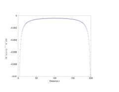
Figure 6: The function $O_{str}=-\langle S^{z}(x)(-1)^{\sum_{j=1}^{x-1}n_{tot}(j)}S^{z}(0)\rangle$ for $U=0$ calculated numerically using the algorithm discussed in appendix A. Here $\rho_{tot}=2{N_{SF}}/{V}=0.2$ and $V=200$. The drawn line is the analytic solution Eq. (45).

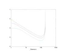
Figure 7: The function $O_{str}=-\langle S^{z}(x)(-1)^{\sum_{j=1}^{x-1}n_{tot}(j)}S^{z}(0)\rangle$ as computed numerically for the free spinful fermion gas at densities $\rho_{tot}=0.2$, $\rho_{tot}=0.6$ and $\rho_{tot}=1$, shown in a log-log plot. The algebraic decay implied by Eq. (45) is indicated by the straight line.

It is obvious where this exponent, equal to unity, is coming from in the calculation. From Eq. (44) it follows that $O_{str}\sim 1/(x^{K_{c,SF}})^{2}$ where the spinless fermion exponent $K_{c,SF}=1/2$. This looks at first sight rather unspectacular but one has to realize that the two point spin correlator of the free-fermion gas decays faster, $\langle SS\rangle\sim 1/x^{2}$ and the topological correlator therefore uncovers a more orderly behavior. Furthermore, the only symmetry reason to expect such an exponent to be equal to unity is the protection coming from $SU(2)$ (spin) symmetry. Can we be certain that this result proves that even in the non-interacting limit a Heisenberg chain is lying within squeezed space? The above computation is not very explicit in this regard and the persuasive evidence is still to come: bosonization, and especially the numerical results presented in section VI showing that the asymptotic behavior of the string correlator is independent of $U$ and density.

V Squeezed spaces and bosonization.

Arriving at this point, we are facing evidence that the squeezed space is actually not at all special to the large $U$ limit. It could well be ubiquitous in one dimensional electron systems. How does bosonization fit in? After all, during the last thirty years overwhelming evidence accumulated for bosonization to be the correct theory in the scaling limit. Squeezed space is of course fundamental; it is among others a precise description of the meaning of spin-charge separation. How could bosonization ever be correct if it would not somehow incorporate the squeezed space structure? In section V.2 we make the case that the peculiarities in the structure of the theory, originating in the core of the bosonization ‘mechanism’ (i.e., the Mandelstam construction for the fermion operators), are just coding for squeezed space. Again, the string operator is the working horse. By just tracking the fate of the string- and two point spin correlators in the bosonization framework, it becomes evident that it is in one-to-one correspondence with the strong coupling limit. This observation is further amplified in Appendix B where we discuss an intuitive argument by Schulz which turns out to subtly misleading. To fix conventions, let us start out collecting some standard expressions.

V.1 The bosonization dictionary.

To fix conventions let us collect here the various standard bosonization expressions we need laterVoitSchulz ; Stone . At the Tomonaga-Luttinger fixed point the dynamics is described in terms of gaussian scalar fields $\varphi_{s}$ and $\varphi_{c}$ for spin and charge, respectively. Introducing conjugate momenta $\Pi_{s,c}$ the Hamiltonian is,

$$\begin{array}[]{rcl}H_{TL}&=&\sum_{\mu=c,s}\frac{v_{\mu}}{2}\int dx\left[K_{\mu}\Pi^{2}_{\mu}+\frac{1}{K_{\mu}}(\partial_{x}\varphi_{\mu})^{2}\right],\end{array}$$ (46)

where $K_{s}$ ($v_{s}$) and $K_{c}$ ($v_{c}$) are the spin and charge stiffness (velocity) respectively. For globally $SU(2)$ symmetric spin systems $K_{s}=1$ and $K_{c}$ is depending on the microscopy, but generally $0\leq K_{c}<1$ for repulsive interactions.

Electron operators can be re-expressed in terms of these bosonic fields via the Mandelstam construction. Starting from the spinful Dirac Hamiltonian describing the linearized electron-kinetic energy,

$$H_{0}=-iv_{F}\sum_{\sigma}\int dx\left[\psi^{\dagger}_{\sigma}(x)\partial_{x}\psi_{\sigma}(x)-\bar{\psi}^{\dagger}_{\sigma}(x)\partial_{x}\bar{\psi}_{\sigma}(x)\right]$$ (47)

The field operators of the left- ($\bar{\psi}_{\sigma}$) and right ($\psi_{\sigma}$) moving fermions are expressed in terms of the bose fields as,

$$\begin{array}[]{rcl}\psi_{\sigma}(x)&=&{{\eta_{\sigma}}\over{\sqrt{2\pi}}}\;e^{i\sqrt{\pi}\left(\varphi(x)-\int_{-\infty}^{x}dy\Pi(y)\right)}\\ \bar{\psi}_{\sigma}(x)&=&{{\bar{\eta}_{\sigma}}\over{\sqrt{2\pi}}}\;e^{-i\sqrt{\pi}\left(\varphi(x)+\int_{-\infty}^{x}dy\Pi(y)\right)}\;,\end{array}$$ (48)

where $\eta_{\sigma},\bar{\eta}_{\sigma}$ are the Klein factors keeping track of the fermion anti-commutation relations.

Starting from the normal ordered charge density the total charge density can be written as,

$$\begin{array}[]{rcl}n_{tot}(x)&=&:n_{\uparrow}(x)+n_{\downarrow}(x):\\ &\simeq&\sqrt{\frac{2}{\pi}}\frac{\partial\varphi_{c}}{\partial x}+{\cal O}_{CDW}(x)+{\cal O}^{\dagger}_{CDW}(x)\;,\end{array}$$ (49)

where $\partial_{x}\varphi_{c}$ represents uniform components of the charge density, while the various finite momentum components are lumped together into $O_{CDW}$. The dominant contributions come from momenta $q=2k_{F}$ and $4k_{F}$,

$$\begin{array}[]{rcl}{\cal O}_{CDW}(x)&=&{\cal O}_{2k_{F}}(x)+{\cal O}_{4k_{F}}(x)\\ {\cal O}_{2k_{F}}(x)&=&\frac{1}{\pi}e^{-2ik_{F}x}e^{i\sqrt{2\pi}\varphi_{c}(x)}\cos\left[\sqrt{2\pi}\varphi_{s}(x)\right]\\ {\cal O}_{4k_{F}}(x)&=&e^{-4ik_{F}x}\frac{1}{2\pi^{2}}e^{i\sqrt{8\pi}\varphi_{c}(x)}\;.\end{array}$$ (50)

Similarly, the spin operator $S^{z}(x)$ becomes,

$$\begin{array}[]{rcl}S^{z}(x)&=&\frac{:n_{\uparrow}(x)-n_{\downarrow}(x):}{2}\\ &=&\sqrt{\frac{1}{2\pi}}\partial_{x}\varphi_{s}(x)+{\cal O}_{SDW,z}(x)+{\cal O}^{\dagger}_{SDW,z}(x)\;,\end{array}$$ (51)

where $\partial_{x}\varphi_{s}$ refers to the uniform (ferromagnetic) component while the finite wavevectors are dominated by the $q=2k_{F}$ component,

$$\begin{array}[]{rcl}{\cal O}^{\dagger}_{SDW,z}(x)&\simeq&{\cal O}_{Sz,2k_{F}}(x)\\ &=&\frac{i}{2\pi}e^{-2ik_{F}x}e^{i\sqrt{2\pi}\varphi_{c}(x)}\sin\left[\sqrt{2\pi}\varphi_{s}(x)\right]\;.\end{array}$$ (52)

In addition we need the usual rules for constructing the propagators of (vertex) operators in a free field theory like Eq. (46),

$$\begin{array}[]{rcl}\langle\partial_{x}\varphi_{\mu}(x)\partial_{x}\varphi_{\nu}(0)\rangle&=&-\delta_{\mu,\nu}{{K_{c}}\over{2\pi}}{1\over{x^{2}}}\\ \langle e^{in\sqrt{2\pi}\left[\varphi_{\mu}(x)-\varphi_{\mu}(0)\right]}\rangle&=&{1\over{x^{n^{2}K_{\mu}}}}\;.\end{array}$$ (53)

V.2 Vertex operators and squeezed space.

It is a peculiarity of bosonization that the charge field enters the spin sector in the form of a vertex operator $\sim e^{i\varphi_{c}}$, see Eq.(52). This can be traced back to the Mandelstam construction for the fermion field operators, Eq. (48), indicating that the fermions are dual to the fields $\varphi$: the fermions have to do with solitons or kinks in the bose fields.

Let us observe the workings of bosonization from the viewpoint offered by the strong coupling limit discussed in section II. We found that the charge-string correlator $D(x)$ is the most fundamental quantity keeping track of the fluctuations in the sublattice parity. Let us see what bosonization has to say about this correlator.

This function becomes in the continuum,

$$\begin{array}[]{rcl}D(x)&\equiv&\langle(-1)^{\sum_{j=0}^{x}n_{tot}(j)}\rangle\\ &=&\langle\cos\left[\pi\sum_{j=0}^{x}n_{tot}(j)\right]\rangle\\ &\rightarrow&\langle\cos\left[\pi\int_{0}^{x}dy~{}n_{tot}(y)\right]\rangle.\end{array}$$ (54)

The theory is constructed to represent the scaling limit and therefore we should focus on the leading singularities. According to Eq.(49), the total charge is given by $n_{tot}=\sqrt{2/\pi}\;\partial_{x}\varphi_{c}$ plus finite $q$ components. One can easily convince oneself that the latter will give rise to subdominant contributions which can be neglected in the scaling limit. Hence,

$$\begin{array}[]{rcl}D(x)&=&\langle\cos\left[\pi\int_{0}^{x}dy\left(\sqrt{2/\pi}\;\partial_{y}\varphi(y)+\cdots\right)\right]\rangle\\ &\rightarrow&\langle\cos\left[\sqrt{2\pi}(\varphi(x)-\varphi(0))\right]\rangle\\ &\sim&{1\over{x^{K_{c}}}}\end{array}$$ (55)

Since bosonization can only probe non-zero wave vector components of the density the expressions are correct up to multiplicative factors $\sim\cos(\pi\rho x)$ ($\rho$ is average density). Keeping this in mind, the outcome is fully consistent with the result obtained for the large $U$ case (Eq. 36, $K_{c}=1/2$ in this limit) but now extended to arbitrary values of the charge stiffness!

The correspondence between bosonization and the strong coupling analysis becomes very obvious in the derivations of the two point spin correlator and the string correlator. Let us recall the standard derivation in bosonization of the spin correlator,

$$\begin{array}[]{rcl}\langle S^{z}(x)S^{z}(0)\rangle&=&\displaystyle\frac{1}{2\pi}\langle\frac{\partial\varphi_{s}(x)}{\partial x}\frac{\partial\varphi_{s}(0)}{\partial x}\rangle+\left[\langle{\cal O}_{SDW,z}(x){\cal O}_{SDW,z}^{\dagger}(0)\rangle+{h.c.}\right]\vspace{1mm}\\ \langle{\cal O}_{SDW,z}(x){\cal O}_{SDW,z}^{\dagger}(0)\rangle&=&\displaystyle\frac{1}{8\pi^{2}}e^{-2ik_{F}x}\langle e^{i\sqrt{2\pi}\left[\varphi_{c}(x)-\varphi_{c}(0)\right]}\rangle\langle e^{i\sqrt{2\pi}\left[\varphi_{s}(x)-\varphi_{s}(0)\right]}\rangle\vspace{1mm}\\ &=&\displaystyle\frac{1}{8\pi^{2}}e^{-2ik_{F}x}\frac{1}{x^{K_{c}+K_{s}}}\end{array}$$ (56)

and the spin-spin correlation function becomes

$$\langle S^{z}(x)S^{z}(0)\rangle=-\frac{K_{s}}{4\pi^{2}}\frac{1}{x^{2}}+\frac{1}{4\pi^{2}}\frac{\cos(2k_{F}x)}{x^{K_{c}+K_{s}}}.$$ (57)

Comparing this with the large $U$ outcome, Eq.’s (38), the correspondence is clear: $\langle e^{i\sqrt{2\pi}\left[\varphi_{s}(x)-\varphi_{s}(0)\right]}\rangle$ is the staggered magnetization of the spin chain in squeezed space, Eq. (21). In strong coupling, the sublattice parity fluctuations enter via the function $\langle n(-1)^{\sum n}n\rangle$ (Eq. 37) which differs from $D$ by just a factor $\cos(\pi\rho x)$. This is of course precisely $e^{-2ik_{F}x}\langle e^{i\sqrt{2\pi}\left[\varphi_{c}(x)-\varphi_{c}(0)\right]}\rangle$ in the bosonization expression Eq. (56). Notice that the subdominant uniform component $\sim 1/x^{2}$ was just ignored in the strong coupling analysis.

The correspondence is further clarified by considering the string correlator. Straightforwardly,

$$\begin{array}[]{rcl}O_{str}(x)&=&-\langle S^{z}(x)(-1)^{\sum_{j=1}^{x-1}n_{tot}(j)}S^{z}(0)\rangle\\ &=&\left(\frac{1}{4\pi}\langle\partial_{x}\varphi_{s}(x)e^{i\sqrt{2\pi}(\varphi_{c}(x)-\varphi_{c}(0))}\partial_{x}\varphi_{s}(0)\rangle+h.c.\right)\\ &&\left(\frac{e^{-2ik_{F}x}}{8\pi^{2}}\langle e^{i\sqrt{2\pi}(\varphi_{c}(x)-\varphi_{c}(0))}e^{-i\sqrt{2\pi}(\varphi_{c}(x)-\varphi_{c}(0))}\rangle\langle e^{-i\sqrt{2\pi}(\varphi_{s}(x)-\varphi_{s}(0))}\rangle+h.c.\right)\\ &&\left(\frac{e^{2ik_{F}x}}{8\pi^{2}}\langle e^{-i\sqrt{2\pi}(\varphi_{c}(x)-\varphi_{c}(0))}e^{-i\sqrt{2\pi}(\varphi_{c}(x)-\varphi_{c}(0))}\rangle\langle e^{-i\sqrt{2\pi}(\varphi_{s}(x)-\varphi_{s}(0))}\rangle+h.c.\right).\\ \end{array}$$ (58)

And these contributions add up to,

$$\begin{array}[]{rcl}O_{str}(x)&=&-\langle S^{z}(x)(-1)^{\sum_{j=1}^{x-1}n_{tot}(j)}S^{z}(0)\rangle\\ &=&-\frac{1}{4\pi^{2}}\frac{1}{x^{2+K_{c}}}-\frac{1}{4\pi^{2}}\frac{\cos(2k_{F}x)}{x^{K_{s}}}-\frac{1}{4\pi^{2}}\frac{\cos(2k_{F}x)}{x^{K_{s}+4K_{c}}}.\end{array}$$ (59)

The first term is obviously the (over corrected) uniform magnetization and the leading singularity at finite wavevectors is,

$$\langle S^{z}(x)(-1)^{\sum_{j=1}^{x-1}n_{tot}(j)}S^{z}(0)\rangle=\frac{\cos(2k_{F}x)}{x^{K_{s}}}.$$ (60)

Again the caveat applies that bosonization cannot keep track of the average charge density and the oscillatory factor in the numerator should therefore be ignored – this ‘flaw’ is just inherited from $D(x)$, Eq. (55). Where is this leading singularity coming from? It corresponds with the third line in Eq. (LABEL:botop1). This algebra is expressing that the charge vertex operator coming from the charge string exactly compensates for the charge vertex operators attached to the spin operators. We recognize that this is in precise correspondence with Eq.’s (24-30) of the strong coupling limit. The charge string is coding for the fluctuating kinks in the sublattice parity and the string correlator is constructed to remove these from the spin correlations.

What have we achieved? The above leaves no doubt that the algebraic structure of bosonization is exactly coding for the structure we discussed in a geometrical language in section III. However, in section III we had to rely on the simplifications arising in the strong coupling limit. The algebraic structure of bosonization is however universal and independent of microscopic conditions like the strength of $U$. For instance, in the non-interacting limit $K_{c}=K_{s}=1$ and one directly infers that the bosonization expressions Eq. (60, 57) are consistent with the exact results we derived for the string- and spin correlators for this limit in section IV. Although there are some caveats regarding the use of bosonization to calculate (charge) string correlators, these are entirely of a technical nature and these affect only subdominant singularities: see appendix B. We can therefore safely conclude that bosonization is just encoding the squeezed space geometrical structure which is manifest in strong coupling. The ‘hard-wired’ structure of bosonization, in combination with the string operators, leaves no room for any other conclusion that squeezed spaces are ubiquitous in Luttinger liquids. It is indeed the case that even non-interacting one dimensional electron systems have deep connections with hidden order in Heisenberg chains.

VI Numerical Results

To verify that the correlator $O_{str}$ indeed demonstrates that squeezed space exists for finite values of the Hubbard coupling $U/t$ and arbitrary density, we performed numerical calculations using the DMRG methodwhite . The DMRG is an ideal tool for these purposes, because the algorithm construction implies that string correlators are, in principle, no more difficult to construct than ordinary two-point correlators. Indeed, the string operator $(-1)^{n_{s}}$ is precisely that which is already used to ensure the correct commutation relations for the creation and annihilation operators. We utilized the non-abelian formulationnonabelian of the DMRG, which makes use of the $SU(2)\otimes SU(2)\simeq SO(4)/Z_{2}$ spin and pseudo-spin symmetry of the Hubbard modelso4 , thereby giving a substantial improvement in efficiency. The pseudo-spin symmetry is an expansion of $U(1)$ particle number symmetry $N$ to an $SU(2)$ symmetry which we denote here by $\vec{Q}$ (this is sometimes also denoted by $\vec{I}$). In the $SO(4)$ representation, the particle-number is given by the $z$-component of the pseudo-spin, $N=2Q^{z}+1$. In our calculation, the basis states are $SO(4)$ multiplets, labeled by two half-integral quantum numbers $(s,q)$ denoting the total spin and total pseudo-spin respectively.

Addressing the scaling limit with the DMRG method is subtle. In the DMRG method, the ground-state wavefunction is calculated in a Hilbert space which is truncated. The parameter controlling the truncation is the number of states kept in each ‘block’, $m$. The actual dimension of the space in which the ground-state wavefunction is determined is of order $(4m)^{2}$. This truncation introduces an error which, for a ‘well-behaved’ system, is completely systematic and can be corrected for by calculating the appropriate scaling as $m\rightarrow\infty$. For the ground-state energy, this scaling is understood and a routine calculation in DMRG. For correlation functions, the scaling is highly non-linear and difficult to perform, not least due to a result highlighted by Östlund and Rommerrommer : the wavefunction obtained by DMRG is a (position-dependent) matrix-product wavefunction, which implies that the long-range asymptotic behavior of all two-point correlation functions is exponential, with a correlation length that depends on the number of states kept $m$. While in principle one can determine this correlation length and fit the remaining (algebraic) components of the correlation function, this is in fact not necessary due to a not so well understood property of (position-dependent) matrix product wavefunctions, namely in the short-distance correlations the exponential due to the finite truncation is not present at all. Thus, as long as a sufficiently large number of states are kept to be close to the scaling limit at distances less than the characteristic transition point where the correlator becomes exponential, the exponents of algebraic terms can be determined with high accuracy without any additional corrections due to the finite truncation.

Also of note is that matrix-product wavefunctions generically carry long-range string order, in the sense that it is likely that all string correlation functions decay exponentially in the asymptotic limit, but it is permissible that the decay is to a non-zero constant. The canonical example is the AKLT wavefunction, which is obtained exactly in (non-abelian) DMRG with $m=1$ states kept. In principle, the variational nature of DMRG implies that for a finite number of states kept one could inadvertently and incorrectly obtain a state that has non-zero string order. This is not a serious issue and is entirely analogous to the case of ordinary two-point correlators which, in the absence of a symmetry constraint, may have a spurious (but usually negligible) non-decaying component. For example, a not-quite-zero uniform magnetization resulting in a non-zero constant in the spin-spin correlator. The point is that the construction of DMRG treats hidden order of the den Nijs-Rommelse type on a very similar footing as more conventional order.

In the calculations presented here, we used $m=1000$ $SO(4)$ states kept, and a lattice size of $L=1000$. The lattice size was chosen to be rather large in an attempt to reduce the effect of the open boundary conditions. However this is not strictly necessary and the usual averaging procedure suffices to eliminate the Friedel oscillations and obtain the correct scaling form of the correlators even for much smaller lattices.

We calculated the string correlator $O_{str}$, Eq. (1), the sublattice parity correlator $D$, Eq. (35) and its second lattice-derivative $D_{nn}$, Eq. (3), for a large variety of filling factors $\rho=0.1\ldots 0.9$ and $U/t=0\ldots 16$. Notice that the number operators appearing in the ‘charge’ strings $D$ and $D_{nn}$ correspond with $n_{s}$ measuring the presence (1) or absence (0) of a singly occupied site. In the exponent one might as well take the total charge density $n_{tot}=n_{\uparrow}+n_{\downarrow}$, i.e. $(-1)^{n_{tot}}=(-1)^{n_{s}}$. However, $D_{nn}\sim\langle n_{s}\Pi(-1)^{n_{s}}n_{s}\rangle\neq\langle n_{tot}\Pi(-1)^{n_{tot}}n_{tot}\rangle$ because $n_{s}$ cannot distinguish empty from doubly occupied sites whereas $n_{tot}$ does. On the bosonization level this subtlety does not matter, but it is consequential for the numerically exact charge string correlators. As the strong coupling analysis in section IV demonstrates, the charge string coding for the squeezed space structure is actually $D_{nn}$ because empty and doubly occupied sites are indistinguishable in the squeezing operation.

The obtained correlation function $O_{str}$ appears in Fig. (8), plotted on a log-log scale. It is clear from the figure that the leading order term in $O_{str}$ is algebraic, with an exponent that is independent of both the filling factor and $U$. The fitted exponent is equal to 1, with a variation over all parameter ranges of $\sim 5\%$. We percieve this as a striking resultLetter , taking away all doubts regarding the ‘universality of squeezed space’: regardless microscopic circumstances we have identified a correlation function which always behaves as if the electron system is just the same spin-chain.

Even the small variation of the exponent is explainable, employing logarithmic corrections. At the $U/t\rightarrow\infty$ Woynarovich-Ogata-Shiba point, the wavefunction factorizes exactly and the $O_{str}$ correlator measures exactly the logarithmic corrections of the isotropic $S=1/2$ antiferromagnetic Heisenberg chainaffleckheis ; Singh . This coincides with the well-known form at half-fillingfinkelstein , where the presence of the charge gap implies Heisenberg-like behavior of the logarithmic corrections for any $U>0$. However, as far as we know, for finite $U/t$ away from half-filling, the exact form of the logarithmic corrections is not known. It is well understood that these corrections are not governed by the conformal field theory, implying that these are non-universal quantities which are sensitive to the short distance dynamics. Hence, they are not necessarily independent of doping and interaction strength. This is confirmed by the non-interacting limit $U=0$ where the system has no log corrections, and there is no reason to expect a discontinuity between $U=0$ and $U\rightarrow\infty$. Therefore we take the scaling form of the string correlator to be

$$O_{str}(x)=A(\rho,U)\frac{\ln^{\alpha}(x)}{x}$$ (61)

and fit for the running exponent $\alpha$. The obtained exponent appears in Fig. (9). We emphasize that this is a very rough calculation, obtained by a direct fit of the finite-size data to the asymptotic form, ignoring finite-size corrections. For the Heisenberg model these corrections are importanthallberg therefore our $U\rightarrow\infty$ estimate of $\alpha\sim 0.25-0.3$, deviates from the exact value of $\alpha=1/2$. Indeed, our result is rather reminiscent of earlier Heisenberg model calculationsscalapino which suffer from similar issues. A careful scaling analysis, done by Hallberg, Horsch and Martinez for the Heisenberg chainhallberg , should present no difficulty and will be reported in a subsequent paper. However, from the present results we can already safely conclude that $\alpha$ is a function of $U/t$ and perhaps also density.

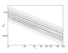
Figure 8: The $O_{str}$ correlator on a log-log plot, for a wide variety of filling and couplings. The slope, which determines the exponent (up to log corrections) of the leading order term, is equal to 1 independent of the parameters.

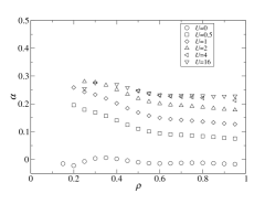
Figure 9: The parameter $\alpha$ governing the logarithmic corrections to $O_{str}$. The logarithmic corrections are very sensitive to finite-size effects, which were not taken into account here. Thus the strong coupling limit deviates from the expected $\alpha=1/2$.

We have argued in previous sections that the charge fluctuations present in the ordinary two-point correlators are due to sublattice parity fluctuations. We found in section III that in the strong coupling limit the following rigorous result holds for the staggered component of the spin-spin correlator,

$$\langle\vec{S}(0)\vec{S}(x)\rangle\sim O_{str}(x)D_{nn}(x)\;.$$ (62)

Our argument is that bosonization reflects this structure and we are now in the position to test this relation numerically for arbitrary values of $U$ and density. As we already emphasized, to isolate the squeezed space the number operators in $D_{nn}$ should measure the density of singly occupied sites, $n_{s}$. In addition, away from the Woynarovich-Ogata-Shiba point Eq. (62) is not longer exact but it should become exact in the scaling limit. Eq. (62) should hold up to a $U,\rho$ dependent prefactor factor which is set by short distance physics. This is exactly what we find. This is demonstrated by Fig. (10) which shows the exponent of the $D_{nn}$ correlator, which turns out to be given by

$$D_{nn}(x)=B(\rho,U)\frac{cos(2k_{F}x)}{x^{K_{c}}}+O(x^{-1-{K_{c}}})\;.$$ (63)

where ${K_{c}}$ is the usual density and $U$-dependent charge stiffness of the Hubbard model. It follows that

$$\langle\vec{S}(0)\vec{S}(x)\rangle=F(\rho,U)\frac{cos(2k_{F}x)}{x^{{K_{c}}+1}}\ln^{\alpha}(x)$$ (64)

coincident with the well known asymptotic behavior of the two point spin correlator in the Luttinger liquid. This completes our case. The fact that we not only isolate the spin-only dynamics in the Luttinger liquid using $O_{str}$ but that we can reconstruct the two point spin correlator by dressing it with an entity which is exclusively counting the sublattice parity mismatches ($D_{nn}$) leaves no doubt that squeezed space is universal.

Let us end this section with giving some numerical results regarding the non universal prefactors $A(\rho,U)$, $B(\rho,U)$ and $F(\rho,U)$. These are clearly sensitive to the details of the short wavelength dynamics and have therefore a similar status as non-universal amplitudes in any critical theory. Hence, these have to be calculated numerically.

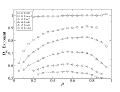
Figure 10: The exponent of $D_{nn}(x)$. This function isolates the charge contribution to the correlation functions, hence gives a direct determination of ${K_{c}}$. The solid lines are guides to the eye.

The prefactor of the $O_{str}$ string correlator, $A(\rho,U)$ is given in figure 11. The numerical prefactor coincides with the expected exact expression at $U=0$ and follows the expected form $\propto\rho$ for $U\rightarrow\infty$, for a Heisenberg chain diluted by a hole density of $(1-\rho)$. The exact slope of the $U\rightarrow\infty$ prefactor depends sensitively on the exponent of the log corrections. The underestimation of $\alpha$ in equation (61) results in the prefactor of figure 11 being somewhat large; the $U\rightarrow\infty$ form should beaffleck

$$O_{str}(x)=\frac{3}{(2\pi)^{3/2}}\frac{\rho\ln^{1/2}(\rho x)}{x}\;.$$ (65)

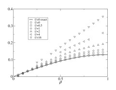
Figure 11: The prefactor of $O_{str}$. The numerical data at $U=0$ matches the exact form determined in section IV. The $U\rightarrow\infty$ prefactor is proportional to the density, exactly as required for a diluted Heisenberg chain.

This differs from the correlator of a stretched Heisenberg chain by a prefactor $\rho^{2}$, which is due to the dilution of the spins; for the Heisenberg chain $\langle s\rangle=1/2$, but for the Hubbard model $\langle s\rangle=n_{s}/2$. Thus, with all prefactors accounted for, the factorization of the $U\rightarrow\infty$ spin correlator isParola ; affleck

$$\begin{array}[]{rcl}\langle\vec{S}(0)\vec{S}(x)\rangle&=&\displaystyle-\frac{3}{4(\pi x)^{2}}+\frac{1}{\rho^{2}}O_{str}(x)D_{nn}(x)\\ &=&\displaystyle-\frac{3}{4(\pi x)^{2}}+\frac{3A^{2}}{(2\pi)^{3/2}}\frac{\cos(2k_{F})}{\rho\sqrt{\sin(2k_{F})}}\frac{\cos(2k_{F}x)\ln^{1/2}(x)}{x^{3/2}}\;,\end{array}$$ (66)

with $2k_{F}=\pi\rho$.

For finite coupling the exact factorization of the wavefunction is destroyed by local fluctations, so Eq. (66) only applies rigorously in the strong coupling limit. As shown in section IV however, the scaling form applies even to $U=0$, with the introduction of a non-universal amplitude $\Gamma(U,\rho)$,

$$\langle\vec{S}(0)\vec{S}(x)\rangle=-\frac{3}{4(\pi x)^{2}}+\Gamma(U,\rho)\,O_{str}(x)\,D_{nn}(x)\;.$$ (67)

Figure 12 shows this amplitude as a function of density and $U$, which is always finite implying that squeezed space is ubiquitous.

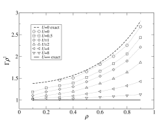
Figure 12: The aplitude $\Gamma$ obtained from $\langle\vec{S}(0)\vec{S}(x)\rangle\sim\Gamma O_{str}(x)D_{nn}(x)$. For clarity plotted as $\Gamma\rho^{2}$, which is equal to unity in the strong coupling limit. The heavy solid and dashed lines are the exact expressions at $U=\infty$ and $U=0$ respectively. The light dashed lines linking the numerical data are guides for the eye.

VII Conclusions: the fermion minus signs.

In first instance the pursuit presented above can be seen as an exploration of the usefulness of string correlators of the den Nijs and Rommelse type in the context of one dimensional physics. To our perception these correlation functions are worthy additions to the standard repertoire of one dimensional physics. This will be further amplified in a next paper where we will further explore the information one can obtain from string correlators like $D$ and $D_{nn}$.

In this paper we used string correlators to clarify some conceptual issues in one dimensional physics. String correlators go hand in hand with the simple geometrical ideas which emerged in the study of Haldane spin chains and the strong coupling Bethe Ansatz solution of the Hubbard model. These correlators make it possible to address to what extent these notions are of relevance to generic Luttinger liquids and we made the case that squeezed spaces are hard-wired into Luttinger liquid theory. It is merely a matter of recognition.

Although complementary to the standard descriptions, we find that the squeezed space notion does exert unifying influences. It is not an accident that we started out discussing the Haldane spin chains. We hope that we convinced the reader that there is a unity underneath which becomes obvious in this language, while it is far from obvious in the standard formulation of bosonization.

Is it more than just clarification? If so, it should be that these insights can be used to deduce states of one dimensional quantum matter which have been overlooked before. In the Luttinger liquid context we have deduced one such novel state: the ‘charge only’ superconductor we introduced at the end of section III. This entity can also be discussed in the bosonization language. It is a prerequisite to drive the system away from critically such that the charge sector is genuinely disordered. This requires an external Josephson field stabilizing superfluid phase order. A conventional Josephson field acting on electrons pairs in the singlet channel is expressed as (recall section V.1),

$$\begin{array}[]{rcl}H_{J}&=&B_{J}\int dx\left(\psi_{\uparrow}(x)\bar{\psi}_{\downarrow}(x)-\psi_{\downarrow}(x)\bar{\psi}_{\uparrow}(x)\right)\\ &\sim&B_{J}\int dx\cos\left[\sqrt{2\pi}\theta_{c}\right]\;\sin\left[\sqrt{2\pi}\varphi_{s}\right]\end{array}$$ (68)

involving the dual charge field $\partial_{x}\theta_{c}(x)=-\Pi(x)$. This imposes phase order (pinning of $\theta_{c}$) but it has also the immediate effect of opening a spin gap ($\sim\sin\left[\sqrt{2\pi}\varphi_{s}\right]$). This spin gap means that the spins are paired in pairwise singlets and a squeezed space cannot be defined for these singlets. Instead, what is required is a Josephson field acting exclusively on the charge fields,

$$H^{\prime}_{J}=B_{J}\int dx\cos\left[\sqrt{2\pi}\theta_{c}\right]$$ (69)

This will enforce disorder on the charge sector, leaving the spin sector unaffected. Recalling the discussion of the spin chain, this charge disorder turns into a $Z_{2}$ gauge invariance in the spin sector. The spin system in squeezed space resides at the ($SU(2)$) critical point separating the XY and Ising fixed points and together with the minimal coupling to the deconfining $Z_{2}$ gauge fields a state of matter is realized which is symmetry-wise indistinguishable from the critical state of the Haldane spin chain found at the transition from the hidden-order phase to the $S=1$ XY phase.

Although such a state is a theoretical possibility, it is less clear whether it can be realized in nature. Bosonization is helpful in clarifying this issue. Starting out with electron operators, it appears to be impossible to construct a Josephson field of the form Eq. (69). One will always find that the charge Josephson field is accompanied by a (relevant) operator in the spin sector. This might well turn out to be a fundamental obstruction. In the one dimensional universe the charge and spin fields are more fundamental than electrons, and a-priori Eq. (69) is physical. However, a Josephson field will in practice correspond with a mean-field coming from three dimensional interactions and this implies that this mean-field has to be a composite of electron degrees of freedom.

As we argued, squeezed space is hard-wired into the bosonization formalism and even exotic states like those discussed in the previous paragraphs are in principle within the reach of the formalism. By implication, if a state of electron matter would exist where squeezed space is destroyed, it would be beyond bosonization. In the context of the (bosonic) spin matter of the Haldane chain we encountered this possibility. Helped by the identification of the $Z_{2}$ gauge symmetry, we presented a recipe (the transversal field) to stabilize a non-squeezed space (‘confining’) phase of the spin chain. Is this also possible in the electron Luttinger liquids?

In this regard it is helpful to view these matters from a yet another angle: the Marshall signs introduced by Weng in the one dimensional contextWeng as an addition to the squeezed space construction needed to describe fermion propagators; see also reference Weng1, for the extension to 2D and for some interesting observations regarding Marshall signs and spin-charge separation in 1D. Marshall signs refer to the theorem that the ground state wave function of a $S=1/2$ spin system defined on a bipartite lattice with nearest neighbor exchange interactions is nodeless: it is a bosonic state. In the strong coupling limit the spin system in squeezed space is of this kind, and this explains in turn why the Bethe-Ansatz solution reveals that the charges are governed by spinless fermions. The total wavefunction has to be anti-symmetric and because squeezed space exists the spin sector is symmetric, so that the fermionic grading resides in the charge sector.

Although we are not aware of an explicit proof, it has to be that this ‘division of statistics’ is universal in the scaling limit. Our string correlator demonstrates that at long distances the squeezed space spin system does behave exactly like the (unfrustrated) Heisenberg chain and it is hard to imagine that this would survive a drastic change involving the nodal structure of the spin wavefunction. Let us assume that the strong coupling limit is in this regard a prototype of any Luttinger liquid, to recollect the lessons learned from the bosonic spin chain. There we learned that to break up squeezed space ‘charge’ fluctuations are needed changing its length from odd to even and vice versa. This implies that single charges can be created or annihilated and this is of course not a problem in a bosonic system because a single boson can condense. However, single fermions cannot condense and since in the Luttinger liquid for reasons just discussed the charge sector is fermionic, confinement is impossible. Admittedly, the argument is circular. It starts out postulating the existence of squeezed space as an entity unfrustrating the spin system in the Marshall sign sense, to find out that the minus signs in turn offer a complete protection of the squeezed space. This viewpoint suggests that there might be ways around the squeezed space and that states can be constructed which are beyond bosonization. Starting from strongly coupled microscopic dynamics, one can image interactions which are strongly frustrating the spin system in the Marshall sign sense (i.e. longer range spin-spin interactions). Such interactions could lead to a ‘signful’ spin physics in squeezed space, which in turn could diminish the ‘statistical protection’, possibly leading to metallic states which are not Luttinger liquids.

A final issue is, is there anything to be learned regarding the relevance of Luttinger liquid physics in higher dimensions? In this paper we have worked hard to persuade the reader that squeezed space is a defining property of the Luttinger liquid. As such, it is a-priori not special to one dimension, in contrast to e.g. the lines of critical points and the Mandelstam construction. Given a complete freedom to choose the microscopic conditions, which fundamental requirements should be fulfilled to form squeezed spaces in higher dimensions? First, bipartiteness is required and this is no longer automatic in higher dimensions. As a starting point one needs a Mott-insulator living on a bipartite lattice characterized by an unfrustrated, colinear antiferromagnet. Upon doping such a Mott-insulator the charges (holes) will frustrate this spin system unless special conditions are fulfilled: these holes have to form $\rm D-1$ dimensional connected manifolds as a fundamental requirement to end up in a bipartite space after the squeezing operation. Different from the one dimensional situation, true long range order will take over when it gets a chance. A first possibility is that these $\rm D-1$ dimensional hole manifolds simply crystallize, forming charge ordered state accompanied by a spin system showing a strong ordering tendency as well, with the characteristic that the staggered order parameter flips every time a charge-manifold is crossed. One immediately recognizes the stripe phases which are experimentally observed in a variety of quasi-2D Mott-insulators, including the cupratesZaanenphilmag . Alternatively, assuming that the holes move in pairs, general reasons are available demonstrating that the charge sector can turn into a superconductor (via a dual dislocation condensationqunematic ) such that the manifolds continue to form domain walls in the sublattice parity although their locus in space is indeterminate. In direct analogy with the Haldane spin chain, such a state is characterized by an emergent ‘sublattice parity’ $Z_{2}$ gauge invariance.

The above is just a short summary of some aspects of the ‘stripe fractionalization’ ideas and for a further discussion we refer to the literatureZaanenphilmag ; Nussinov ; Sachdev0 ; Sachdev1 . Most importantly, the notion of squeezed space make it clear why ‘Luttinger liquid-like’ physics is not at all generic in higher dimensions but instead rather fragile, if it exists at all. The bipartiteness of squeezed space-time in the space directions has to be protected and this requires microscopic fine-tuning.

The punchline is that if one wants to contemplate manifestations of Luttinger liquid physics in higher dimensions it must be striped in one way or the other, since squeezed spaces are the most precise way to characterize the phenomenon of spin-charge separation as it arises in the specific one dimensional context. This insight also makes is clear why attempts to invoke the equations governing the Luttinger liquids in whatever phenomenological spirit to explain physics in higher dimensions are bound to fail: these represent a dynamics which is slaved to an underlying geometrical principle which is only of the right kind in one space dimension. To bosonize the electron itself in two space dimensions one has to invoke geometrical/gauge principles of a fundamentally different kindFradkin ; Weng1 .

Appendix A Computation of the charge string correlator of free spinless fermions.

In this appendix we discuss the numerical computation of the free spinless fermion charge string operator, Eq.(35). We find that it can be fitted very accurately with the simple expression Eq. (36). This may well be an exact result but we did not manage to find the solution with analytical means.

Using periodic boundary conditions, the charge string correlator can be written as

$$\begin{array}[]{rcl}\langle\,(-1)^{\sum_{j=1}^{x-1}n(j)}\rangle&=&\langle k_{N}\ldots k_{1}|(-1)^{\sum_{j=1}^{x-1}n_{SF}(j)}\,|k_{1}\ldots k_{N}\rangle_{SF}\\ &=&\sum_{x_{1}\ldots x_{N}}\sum_{y_{1}\ldots y_{N}}\langle 0|a_{x_{N}}\ldots a_{x_{1}}(-1)^{\sum_{j=1}^{x-1}n(j)}a_{y_{1}}^{\dagger}\ldots a_{y_{N}}^{\dagger}|0\rangle\\ &&\times\left(\frac{1}{V}\right)^{N}e^{-ik_{1}x_{1}-\ldots-ik_{N}x_{N}}~{}e^{ik_{1}y_{1}+\ldots+ik_{N}y_{N}}\\ &=&\sum_{x_{1}\ldots x_{N}}\sum_{y_{1}\ldots y_{N}}\langle 0|a_{x_{N}}\ldots a_{x_{1}}a_{y_{1}}^{\dagger}\ldots a_{y_{N}}^{\dagger}|0\rangle\\ &&\times\left(\frac{1}{V}\right)^{N}e^{-ik_{1}x_{1}-\ldots-ik_{N}x_{N}}~{}e^{ik_{1}y_{1}+\ldots+ik_{N}y_{N}}\\ &&\times\prod_{j=1}^{N}\left[1-2\theta(y_{j}-1)\theta(r-1-y_{j})\right]\;.\end{array}$$ (70)

occupying the lowest N $|k_{1}\ldots k_{N}\rangle$ single fermion states. The product term on the last line equals $-1$ when $y_{j}\in\left[1,x-1\right]$ and 1 otherwise, taking into account the result of the factor $(-1)^{\sum_{j=1}^{x-1}n_{SF}(j)}$. Part of this sum can be written as

$$\frac{1}{V}\sum_{y}e^{iy(p-k)}\left[1-2\theta(y-1)\theta(x-1-y)\right] = \frac{1}{V}\sum_{y}e^{iy(p-k)}-\frac{2}{V}\sum_{y=1}^{x-1}e^{iy(p-k)}$$ (71)

$$= \delta(p,k)-\frac{2}{V}\frac{e^{i(p-k)x}-e^{i(p-k)}}{e^{i(p-k)}-1}$$

$$\equiv \delta^{*}(p,k),$$

abbreviating the second line with the ‘star-delta function’ $\delta^{*}(p,k)$. Using this function, the expression (70) can be expressed as the determinant of a $N\times N$ matrix containing $\delta^{*}(k_{i},k_{j})$ functions

$$\langle(-1)^{\sum_{j=1}^{x-1}n_{SF}(j)}\rangle=\mbox{det}\left(\begin{array}[]{cccc}\delta^{*}(k_{1},k_{1})&\delta^{*}(k_{2},k_{1})&\cdots&\delta^{*}(k_{N},k_{1})\\ \delta^{*}(k_{1},k_{2})&\delta^{*}(k_{2},k_{2})&\cdots&\delta^{*}(k_{N},k_{2})\\ \delta^{*}(k_{1},k_{3})&\delta^{*}(k_{2},k_{3})&\cdots&\delta^{*}(k_{N},k_{3})\\ \vdots&\vdots&\vdots&\vdots\\ \delta^{*}(k_{1},k_{N})&\delta^{*}(k_{2},k_{N})&\cdots&\delta^{*}(k_{N},k_{N})\\ \end{array}\right).$$ (72)

and this determinant can be straightforwardly computed numerically for a finite system.

Careful analysis of the numerical data for a complete range of densities, demonstrates that,

$$\langle\,(-1)^{\sum_{j=1}^{x-1}n(j)}\,\rangle_{SF}=\frac{A^{2}\sqrt{2}}{\sqrt{\sin(\frac{\pi N}{V})}}\frac{\cos(\frac{\pi(x-1)N}{V})}{\sqrt{\frac{V}{\pi}\sin(\frac{\pi(x-1)}{V})}}\;.$$ (73)

As an example, in Fig. (13) we show results for $\rho_{SF}=\frac{N}{V}=0.1$ for $N=20$ particles on a chain of length $V=200$ and this compared with the analytic expression (73). In Fig. (14) the numerical outcomes for the prefactor of $\langle(-1)^{\sum_{j=1}^{x-1}n_{SF}(j)}\rangle$ taking a normalization such that this prefactor is 1 for $\rho_{SF}=\frac{N}{V}=0.5$. According to the exact result by Parola and SorellaParola this prefactor is equal to $\langle(-1)^{\sum_{j=1}^{x-1}n_{SF}(j)}\rangle\sqrt{\frac{V}{\pi}\sin(\frac{\pi(x-1)}{V})}/(A^{2}\sqrt{2}\cos(\frac{\pi(x-1)N}{V}))$. The perfect match between this normalized numerical outcome and the function $\frac{1}{\sqrt{\sin(\pi\rho_{SF})}}$ establishes the density dependence of the amplitude in Eq. (73).

In the thermodynamic limit $V\rightarrow\infty,\frac{N}{V}\rightarrow\rho_{SF}$ Eq. (73) becomes,

$$\langle\,(-1)^{\sum_{j=1}^{x-1}n(j)}\,\rangle_{SF}=\frac{A^{2}\sqrt{2}}{\sqrt{\sin(\pi\rho_{SF})}}\frac{\cos(\pi\rho_{SF}(x-1))}{\sqrt{x-1}}.$$ (74)

reproducing the exact result by Parola and SorellaParola at the density $\rho_{SF}=\frac{1}{2}$. These authors showed that at this specific density the asymptotic form of $D(x)$ is

$$D(x)=\langle\,(-1)^{\sum_{j=0}^{x}n_{SF}(j)}\,\rangle=A^{2}\sqrt{2}\frac{\cos(\frac{\pi(x+1)}{2})}{\sqrt{x+1}},$$ (75)

Figure 13: Numerical results (circles) for the function $D(x)=\langle(-1)^{\sum_{j=0}^{x}n_{SF}(j)}\rangle$ calculated from (72), as compared to the analytical form Eq. (73) (full line) This is a representative example: we use $N=20$ particles on on a chain of length $V=200$ (density $\rho_{SF}=\frac{N}{V}=0.1$), using periodic boundary conditions.

density $\rho_{SF}=\frac{N}{V}=0.1$.

Figure 14: The crosses indicate the numerical results for the prefactor of the function $D(x)=\langle(-1)^{\sum_{j=0}^{x}n_{SF}(j)}\rangle$ normalized to 1 for $n=\rho_{SF}=\frac{N}{V}=0.5$ ($V=200$). The full line corresponds with the function $\frac{1}{\sqrt{\sin(\pi\rho_{SF})}}$.

For completeness, let us list the outcomes for the expectation values $\langle n(x)(-1)^{\sum_{j=1}^{x-1}n(j)}\rangle_{S}F$ and $\langle\,n(x)(-1)^{\sum_{j=1}^{x-1}n(j)}n(0)\rangle$ which can be regarded as lattice derivatives of the charge string correlator Eq. (74). Eg find

$$\begin{array}[]{rcl}\lx@intercol\@ADDCLASS{ltx_eqn_lefteqn}$\displaystyle\langle\,n(x)\,(-1)^{\sum_{j=1}^{x-1}n(j)}\,\rangle_{SF}\,$\mbox{}\hfil\lx@intercol~{}~{}~{}\\ &=&\langle\,(-1)^{\sum_{j=1}^{x-1}n(j)}\,n_{SF}(0)\,\rangle_{SF}\,=\frac{D(x-2)-D(x-1)}{2}\\ &=&\frac{A^{2}}{\sqrt{2\sin(\pi\rho_{SF})}}\left(\frac{\cos(\pi\rho_{SF}x)\left[\cos(\pi\rho_{SF})-1\right]+\sin(\pi\rho_{SF}x)\sin(\pi\rho_{SF})}{\sqrt{x}}\right)\\ &=&\mbox{sign}\left[\cos(\pi\rho_{SF})-1\right]\frac{A^{2}\sqrt{1-\cos(\pi\rho_{SF})}}{\sqrt{\sin(\pi\rho_{SF})}}\frac{\cos(\pi\rho_{SF}x-K)}{\sqrt{x}}\;,\end{array}$$

where the constant $K$ is given by

$$K=\frac{\pi(\rho-1)}{2}\;.$$ (76)

In addition,

$$\begin{array}[]{rcl}\langle\,n(x)\,(-1)^{\sum_{j=1}^{x-1}n(j)}\,n(0)\,\rangle_{SF}&=&\displaystyle\frac{1}{4}\left[D(x-2)-2D(x-1)+D(x)\right]\vspace{1mm}\\ &=&\displaystyle\frac{A^{2}(\cos(\pi\rho_{SF})-1)}{\sqrt{2\sin(\pi\rho_{SF})}}\frac{\cos(\pi\rho_{SF}x)}{\sqrt{x}}\;.\end{array}$$ (77)

Appendix B A caveat: Schulz’ flawed logic.

The idea that the charge fluctuates the space in which the spin system resides has a long history. In this appendix we would like to comment on an argument due to the late Heinz SchulzSchulz1 . His argument is not correct, but the flaw is subtle and informative regarding the workings of sublattice parity fluctuations.

In the above, we re-derived the ‘classic’ result that the two point spin correlator $\langle SS\rangle\sim 1/x^{K_{c}+K_{s}}$. SchulzSchulz1 asserted that this behavior can be explained by assuming that the system can be seen as a 1+1D harmonic crystal of charges in the continuum. The spins at the sites of this crystal would just form a Heisenberg antiferromagnet. True long range crystal order is impossible in 1+1D because the admixture of the Goldstone bosons (phonons) renders the correlations to be algebraic (algebraic long range order, ALRO). Schulz’ idea was simple: the spin systems does not live on fixed positions in space but instead on a medium undergoing gaussian fluctuations, as if the spin system ‘surfs’ on the gaussian charge waves.

The effects on the spin correlator can be easily calculated. In the continuum the spin density equals

$$\vec{S}(x)=\sum_{m}\vec{S}_{Heis.}(m)\delta(x-x_{m}),$$ (78)

summing over all the electrons. Starting from the ALRO crystal, $x_{m}$ can be written as $x_{m}=R_{m}+u_{m}$, where $R_{m}=\frac{m}{\rho}$ is the position in the $m$-th electron and $u_{m}$ its displacement. One finds for the correlation function,

$$\langle\vec{S}(x)\vec{S}(0)\rangle\sim\int dq\sum_{m,m^{\prime}}e^{-iqx}\langle\vec{S}_{Heis.}(m)\vec{S}_{Heis.}(m^{\prime})\rangle e^{iq(R_{m}-R_{m^{\prime}})}\langle e^{iq(u_{m}-u_{m^{\prime}})}\rangle\;.$$ (79)

Due to the gaussian fluctuations,

$$\langle e^{iq(u_{m}-u_{m^{\prime}})}\rangle\approx|m-m^{\prime}|^{-\alpha(q)},$$ (80)

with $\alpha(q)\sim q^{2}$. The $q$ integration in Eq. (79) is dominated by the term $q\approx\pi\rho=2k_{F}$ and using the Heisenberg correlation function, Eq. (21),

$$\langle\vec{S}(x)\vec{S}(0)\rangle \approx \int dq\sum_{m,m^{\prime}}e^{iq(R_{m}-R_{m^{\prime}}-x)}\langle\vec{S}_{Heis.}(m)\vec{S}_{Heis.}(m^{\prime})\rangle|m-m^{\prime}|^{-\alpha(2k_{F})}$$ (81)

$$\approx \int dq\sum_{m,m^{\prime}}e^{iq(\frac{m}{\rho}-\frac{m^{\prime}}{\rho}-x)}\frac{(-1)^{m-m^{\prime}}}{|m-m^{\prime}|^{1+\alpha(2k_{F})}}$$

$$= \frac{\cos(\pi\rho x)\ln^{1/2}(\rho x)}{(\rho x)^{1+\alpha(2k_{F})}}=\frac{\cos(2k_{F}x)}{(\rho x)^{1+\alpha(2k_{F})}}\ln^{1/2}(\rho x).$$

This outcome looks indeed quite like the desired result, identifying $\alpha(2k_{F})$ with $K_{c}$ . However, this similarity is actually misleading! Schulz’ crystal refers to the breaking of translation symmetry by single electron charges. Implicitly, this refers to the strongly coupled regime considered in the above and this crystal corresponds with the spinless-fermion ALRO crystal (e.g. reference Zaanenstr, ). The spinless fermion $2k_{F}$ turns into a spinful electron $4k_{F}$ wave vector. Accordingly, the exponent $\alpha(2k_{F})$ should be associated with the charge stiffness appearing in the $4k_{F}$ charge correlations, and this stiffness is not $K_{c}$ but instead $4K_{c}$! For instance, in the large $U$ case $K_{c}=1/2$ and the Schulz argument would predict that the spin correlations would decay like $1/x^{3}$ instead of $1/x^{3/2}$.

Where is the flaw? In fact, the implicit assertion in the above is that $\langle SS\rangle\sim\langle\;n\;n\;\rangle_{4k_{F}}\times\langle SS\rangle_{Heis.}$. We learned, however, that the geometry of the spin system is fluctuated by kinks in their translational sector (the sublattice parity flips). These are dual to the charge-order and one has to use instead the exponentiated charge strings $\langle SS\rangle\sim\langle n(-1)^{\sum n}n\rangle\times\langle SS\rangle_{Heis.}$. As we showed, $\langle n(-1)^{\sum n}n\rangle$ decays with an exponent which is $K_{c}$ itself. From the discussion in section IV it is clear that this dual structure is in fact respected by bosonization. In this sense, bosonization ‘knows’ about squeezed space.

References

- (1) J. Voit Rep. Prog. Phys. 58, 977 (1995); H. J. Schulz, G. Cuniberti and P. Pieri in Field Theories for Low-Dimensional Condensed Matter Systems, G. Morandi et al, Eds. Springer (2000), cond-mat/9807366.
- (2) M. Stone, Bosonization, World Scientific (1994); S. Rao and D. Sen, cond-mat/0005492; J. von Delft and H. Schoeller, cond-mat/9805275; R. Shankar, Acta Phys. Pol B26, 1835 (1995).
- (3) C. Dekker, Physics Today 52(5), 22 (1999).
- (4) H.V. Kruis, I.P. McCulloch, Z. Nussinov and J. Zaanan, Europhys. Lett. (in press, cond-mat/0209493).
- (5) M. den Nijs and K. Rommelse, Phys. Rev. B, 40, 4709 (1989).
- (6) C. D. Batista and G. Ortiz, Phys. Rev. Lett. 86, 1082 (2001).
- (7) J. Zaanen, O.Y. Osman, H.V. Kruis, Z. Nussinov and J. Tworzydlo, Phil. Mag. B 81, 1985 (2002).
- (8) Z. Nussinov and J. Zaanen, J. Phys. IV France, 12, Pr9-245 (2002); J. Zaanen and Z. Nussinov, Phys. Stat. Sol. B 236, 332 (2003).
- (9) Y. Zhang, E. Demler and S. Sachdev, Phys. Rev. B. 66, 094501 (2002).
- (10) S. Sachdev, Rev. Mod. Phys. 75, 913 (2003); Ann. Phys. (NY) 303, 226 (2003).
- (11) J. Zaanen and O. Gunnarsson, Phys. Rev. B 40, 7391 (1989).
- (12) S.A. Kivelson, E. Fradkin, V. Oganesyan, I.P. Bindloss, J. M. Tranquada, A. Kapitulnik and C. Howald, Rev. Mod. Phys. (in press) (cond-mat/0210683).
- (13) F. Woynarovich, J. Phys. C 15, 85 (1982); ibid. 15, 96 (1982).
- (14) M. Ogata and H. Shiba, Phys. Rev. B 41, 2326 (1990).
- (15) F.D.M. Haldane, Phys. Rev. Lett. 50, 1153 (1983).
- (16) I. Affleck, T. Kennedy, E.H. Lieb and H. Tasaki, Com. Math. Phys. 115, 477 (1988).
- (17) H. Tasaki, Phys. Rev. Lett. 66, 798 (1991).
- (18) H. Eskes, O.Y. Osman, R. Grimberg, W. van Saarloos and J. Zaanen, Hys. Rev. B 58, 6963 (1998); H. Eskes, R. Grimberg, W. van Saarloos and J. Zaanen, Phys. Rev. B 54, R724 (1996).
- (19) T. Senthil and M.P.A. Fisher, Phys. Rev. B 62, 7850 (2000).
- (20) J. B. Kogut, Rev. Mod. Phys. 51, 659 (1979).
- (21) E. H. Lieb and F. Y. Wu, Phys. Rev. Lett. 20, 1445 (1968).
- (22) A. Parola and S. Sorella, Phys. Rev. Lett. 64, 1831 (1990).
- (23) J. Zaanen and W. van Saarloos, Physica C 282, 178 (1997).
- (24) R. Resta, Phys. Rev. Lett. 80, 1800 (1998); R. Resta and S. Sorella, Phys. Rev. Lett. 82, 370 (1999); M. Nakamura and J. Voit, Phys. Rev. B 65, 153110 (2002).
- (25) J.C. Talstra, S.P. Strong and P.W. Anderson, Phys. Rev. Lett. 74, 5256 (1995); S.P. Strong and J.C. Talstra, Phys. Rev. B 59, 7362 (1999).
- (26) R. R. P. Singh, M. E. Fisher and R. Shankar, Phys. Rev. B, 39, 2562 (1989).
- (27) S. R. White, Phys. Rev. Lett. 69, 2863 (1992); Phys. Rev. B 48, 10, 345 (1993).
- (28) I. P. McCulloch and M. Gulácsi, Euro. Phys. Lett. 57, 852 (2002).
- (29) C. N. Yang and S. C. Zhang, Mod. Phys. Lett. B4, 759 (1990).
- (30) S. Östlund and S. Rommer, Phys. Rev. Lett. 75, 3537 (1995).
- (31) I. Affleck, D. Gepner, H. J. Schulz and T. Ziman, J. Phys. A 22, 511 (1989).
- (32) A. M. Finkel’shteĭn, JETP Lett. 25, 73 (1977) [Pis’ma Zh. Eksp. Teor. Fiz. 25, 83 (1977)]
- (33) K. A. Hallberg, P. Horsch and G. Martinez, Phys. Rev. B 52, R719 (1995).
- (34) For example: K. Kubo, T. A. Kaplan and J. Borysowicz, Phys. Rev. B 38, 11550 (1988); S. Liang, Phys. Rev. Lett 64, 1597 (1990).
- (35) I. Affleck, J. Phys. A 31, 4573 (1998)
- (36) Z.Y. Weng, Phys. Rev. B 50, 13837 (1994); Z.Y. Weng, D.N. Sheng, C.S. Ting and Z.B. Su, Phys. Rev. B 45, 7850 (1992).
- (37) Z.Y. Weng, D.N. Sheng, Y.-C. Chen, and C.S. Ting, Phys. Rev. B 55, 3894 (1997).
- (38) J. Zaanen, Z. Nussinov and S.I. Mukhin, Ann. Phys. (NY) in press (cond-mat/0309397).
- (39) E. Fradkin, Phys. Rev. Lett. 63, 322 (1989).
- (40) H. J. Schulz, cond-mat/9412036.
- (41) For example: J. Zaanen, Phys. Rev. Lett. 84, 753 (2000).