$O{(N)}$ algorithms for disordered systems

Abstract

The past thirteen years have seen the development of many algorithms for approximating matrix functions in $O{(N)}$ time, where $N$ is the basis size. These $O{(N)}$ algorithms rely on assumptions about the spatial locality of the matrix function; therefore their validity depends very much on the argument of the matrix function. In this article I carefully examine the validity of certain $O{(N)}$ algorithms when applied to hamiltonians of disordered systems. I focus on the prototypical disordered system, the Anderson model. I find that $O{(N)}$ algorithms for the density matrix function can be used well below the Anderson transition (i.e. in the metallic phase;) they fail only when the coherence length becomes large. This paper also includes some experimental results about the Anderson model’s behavior across a range of disorders.

00000000

V. E. Sacksteder $O{(N)}$ algorithms for disordered systems

vincent@sacksteder.com

1 INTRODUCTION

Certain matrix functions - the Green’s function, the density matrix, and the logarithm - are very important to science and engineering. Where they are important, scientists are faced with a computational bottleneck: evaluation of a matrix function generally requires $O{(N^{3})}$ time, where $N$ is the basis size and usually scales linearly or worse with the system volume. This prohibits computations of large systems, even with modern computers. In particular, if a matrix function must be recalculated at every step of a system’s evolution in time, then calculations with a basis size larger than $O{(1000-10000)}$ are not practical.

In 1991 W. Yang introduced the Divide and Conquer algorithm, which approximated a matrix function in $O{(N)}$ time[21]. This stimulated the development of many other $O{(N)}$ algorithms [1, 2, 11] which have met considerable success, permitting for instance quantum dynamics calculations of tens of thousands of atoms. All $O{(N)}$ algorithms rely on special characteristics of the system under study, and the question of their validity can be answered only after having specified that system. To date, theoretical studies of the validity of these algorithms have occurred almost exclusively within the conceptual framework of ordered systems, using ideas of metals, insulators, and band gaps[6, 7, 8, 9, 10, 11, 12, 13, 14, 15]. In this paper I carefully examine the applicability of $O{(N)}$ algorithms to disordered systems. I calculate a matrix function in two ways: with an $O{(N)}$ algorithm, and via diagonalization. Comparison of the two results provides some new insight into when disorder can make $O{(N)}$ calculations feasible.

This paper begins by introducing $O{(N)}$ algorithms (section 2) and then explaining how to measure the errors which these algorithms induce (section 3.) Section 4 introduces disordered systems and the density matrix function, while section 5 gives theoretical estimates of $O{(N)}$ errors. I present my numerical results in section 6, and finish in section 7 with a short assessment of their reliability.

2 O(N) Algorithms

All $O{(N)}$ algorithms make three basic assumptions:

• Existence of a Preferred, Local Basis. It is assumed that the system is best described in terms of a localized basis set. I here define a basis as localized if for any basis element ${|\psi\rangle}$, only a small number of positions $\vec{x}$ satisfy ${\langle\vec{x}|\psi\rangle}\neq 0$.

• Existence of a Distance Metric. There must be a way of computing the physical distance between any two basis elements ${|\psi\rangle}$ and ${|\acute{\psi}\rangle}$.

• Locality of both the Matrix Function and its Argument. I call a matrix $A$ local if, for every pair of basis elements $|\vec{x}\rangle$ and $|\vec{y}\rangle$ that are far apart, ${{\langle\vec{x}|}A{|\vec{y}\rangle}}=0$. Throughout this article I choose a simple criterion for being far apart: comparison with a radius $R$.

There are a number of ways for an $O{(N)}$ algorithm to exploit the three basic assumptions. In this article I focus on the class of algorithms based on basis truncation. This class includes Yang’s Divide and Conquer algorithm[21], the ”Locally Self-Consistent Multiple Scattering” algorithm[3, 4], and Goedecker’s ”Chebychev Fermi Operator Expansion”[22, 23], which I will henceforth call the Goedecker algorithm. Basis truncation algorithms break the matrix function into spatially separated pieces. Given the position of a particular piece, the basis is truncated to include only elements close to that position, and then the matrix function is calculated within the truncated basis. Thus, for any generic matrix function $f{(H)}$, a basis truncation algorithm calculates ${{\langle\vec{x}|}{f{(H)}}{|\vec{y}\rangle}}={{\langle\vec{x}|}{f{(P_{\vec{x},\vec{y}}HP_{\vec{x},\vec{y}})}}{|\vec{y}\rangle}}$, where $P_{\vec{x},\vec{y}}$ is a projection operator truncating all basis elements far from $\vec{x}$, $\vec{y}$. There may be also an additional step of interpolating results obtained with different $P$’s, but I will ignore this. In this paper I choose $P$ to be independent of the left index $\vec{x}$, and truncate all basis elements outside a sphere of radius $R$ centered at $\vec{y}$.

Basis truncation algorithms vary only in their choice of how to evaluate the function ${f{(P_{\vec{x},\vec{y}}HP_{\vec{x},\vec{y}})}}$. Specifically, Yang’s algorithm calculates $f$ in terms of the argument’s eigenvectors, the Goedecker algorithm does a Chebyshev expansion of $f$, and the ”Locally Self-Consistent Multiple Scattering” algorithm calculates the argument’s resolvent or Green’s function and then obtains $f$ via complex integration. Because these approaches are all mathematically equivalent when applied to analytic functions, they should all converge to identical results, as long as one makes identical choices of which matrix function to evaluate, of how to break up the function, of which projection operator to use, and of a possible interpolation scheme. Moreover, given an identical choice of matrix function, variations in the other choices should obtain results that are qualitatively the same. In this paper I use the Goedecker algorithm, but I want to emphasize that the results obtained here apply to the whole class of basis truncation algorithms.

The Goedecker algorithm is essentially a Chebyshev expansion of the matrix function. As long as all the eigenvalues of the argument $H$ are between $1$ and $-1$, a matrix function may be expanded in a series of Chebyshev polynomials of $H$: $f{(H)}\cong{\sum_{s=0}^{S}{c_{s}T_{s}{(H)}}}$. The coefficients $c_{s}$ are independent of the basis size, and therefore can be calculated numerically in the scalar case. The Chebyshev polynomials can be calculated in $O{(N)}$ time using the recursion relation $T_{s+1}={{({2HT_{s}})}-T_{s-1}}$, $T_{1}=H$, $T_{0}$ = 1. (Of course, one must also bound the highest and lowest eigenvalues of $H$ and then normalize. In practice very simple heuristics are sufficient for estimating these bounds.) If the matrix function $f{(H)}$ has a characteristic scale of variation $\alpha$, then the error induced by the Chebyshev expansion is controlled by an exponential with argument of order $-\alpha S$.

3 Measuring The Error

Previous efforts to test numerically the accuracy of $O{(N)}$ algorithms have been confined to evaluations of whether the overall physical predictions are reasonable, and tests of convergence with respect to the localization radius $R$ and any other parameters. In contrast, in this paper I compute a matrix function using both an $O{(N)}$ algorithm and an algorithm based on diagonalization, and then compare the results.

This careful comparison required development of a metric for comparing two matrices. First, note that the dot product used for comparing two vectors can be easily generalized to matrices:

$${MDP{(A,B)}}\equiv{Tr{(AB)}}={\sum_{\vec{x},\vec{y}}{{\langle\vec{x}|A|\vec{y}\rangle}{\langle\vec{y}|B|\vec{x}\rangle}}}$$

If $A=B$, this matrix dot product is just square of the Frobenius norm, one of the traditional norms for matrices. Note also that matrix dot product is invariant under change of basis. Moreover, it is simple to show that ${-1}\leq{\frac{MDP{(A,B)}}{\sqrt{{MDP{(A,A)}}{MDP{(B,B)}}}}}\leq{1}$, so one may define the angle $\theta$ between two matrices as the arcsin of this quantity. Bowler and Gillan[24] justified this, showing that the concept of perpendicular and parallel matrices is valid and useful.

However the matrix dot product is not quite suited to my needs. $O{(N)}$ algorithms have a preferred, local basis, and thus are not well matched by a basis invariant measure. Moreover, the matrix functions which they compute are expected to agree best with the exact matrix functions close to the diagonal, and to agree not at all outside the truncation radius. Therefore, a more sensitive metric is needed, one that distinguishes different distances from the diagonal. I define the Partial Matrix Dot Product as:

$${MDP{(A,B,\vec{x})}}\equiv{\sum_{\vec{y}}{{\langle\vec{y}|A|{\vec{y}+\vec{x}}\rangle}{\langle\vec{y}|B|{\vec{y}+\vec{x}}\rangle}}}$$

The argument $\vec{x}$ of this dot product allows me to obtain information about agreement at displacement $\vec{x}$ from the diagonal. It is still valid to call this a dot product, because the magnitude of $\frac{MDP{(A,B,\vec{x})}}{\sqrt{{MDP{(A,A,\vec{x})}}{MDP{(B,B,\vec{x})}}}}$ is bounded by one, and thus one can compute a displacement-dependent angle $\theta{(\vec{x})}$ and relative magnitude $m{(\vec{x})}$. The partial matrix dot product has a simple sum rule relating it to the full matrix dot product: $MDP{(A,B)}={\sum_{\vec{x}}{MDP{(A,B,\vec{x})}}}$.

In my results I actually compute another dot product, an angular average $MDP{(A,B,r)}$ over all $\vec{x}$ satisfying ${r}={|\vec{x}|}$.

4 The Density Matrix

In this paper I restrict my attention to a single matrix function, the density matrix. This function is very important in quantum calculations of electronic structure in atoms and molecules, where its argument is the system’s Hamiltonian, its diagonal elements describe the charge density, and its off-diagonal elements are used to compute forces on the atoms. Eigenvalues of the Hamiltonian give the energies of their corresponding electronic states, and I will use the words eigenvalue and energy interchangeably throughout the rest of this paper.

The density matrix function $\rho{(\mu,T,H)}$ is basically a projection operator which deletes eigenvectors having energy $E$ larger than the Fermi level $\mu$. Here I use the following form:

$$\rho{(\mu,T,H)}={\frac{1}{2}{Erfc}{(\sqrt{2}{(\frac{H-{\mu I}}{T})})}}$$

For physical reasons, it is not quite a projection operator: it has a transition region around $\mu$ of width proportional to the temperature $T$ where its eigenvalues interpolate between $0$ and $1$. The error induced by a Chebyshev expansion is controlled by an exponential with argument proportional to ${-TS}/{\Delta}$, where $\Delta$ is the size of the energy band and $S$ is the number of terms in the Chebyshev expansion[22].

The density matrix is well suited to $O{(N)}$ algorithms. As $\mu$ becomes large, it converges to the identity. Moreover, it is invariant under unitary transformations acting on the set of eigenvectors with energies below the Fermi level[2]. Even when the Hamiltonian’s eigenvectors are not a local basis set, often a unitary transformation can be found which maps them to a basis which is localized. If such a transformation exists, the density matrix is localized.

Several papers have examined density matrix locality in the context of ordered systems; i.e. ones whose Hamiltonians possess lattice translational invariance[6, 7, 8, 9, 10, 11, 12, 13, 14, 15]. (Lattice translational invariance can be expressed quantitatively as ${{\langle\vec{x}|}H{|\vec{y}\rangle}}={{\langle\vec{x}+\vec{\Delta}|}H{|\vec{y}+\vec{\Delta}\rangle}}$ for all $\vec{\Delta}$ located on an infinitely extended lattice.) It is well known that the eigenvalues of such systems are arranged in bands separated by energy gaps where there are no eigenvalues, and that the eigenvectors are extended through all space. Notwithstanding the nonlocality of the eigenvectors, there are strong arguments for localization in all ordered systems. If the system is metallic (meaning that the Fermi level lies in one of the bands of eigenvalues) and the temperature is zero, then in a three-dimensional system the density matrix is expected to fall off asymptotically as ${R^{-2}}$, where $R$ is the spatial distance from the diagonal. A non-zero temperature multiplies this by an exponential decay. If instead the system is an insulator, then the density matrix should decay exponentially even at $T=0$.

Most systems of physical interest do not exhibit lattice translational symmetry. In particular, many exhibit inhomogeneities at scales much smaller than that of the system itself. These are termed disordered systems. In this article I study the prototypical disordered system, the Anderson model[18]. It describes a basis laid out on a cubic lattice, one basis element per lattice site, and a very simple symmetric Hamiltonian matrix $H$ composed of two parts:

• A regular part: ${\langle\vec{x}|H|\vec{y}\rangle}=1$ if $\vec{x}$ and $\vec{y}$ are nearest neighbors on the lattice. This term is, up to a constant, just the second order discretization of the Laplacian; its spectrum consists of a single band of energies between $-2D$ and $2D$, where $D$ is the spatial dimensionality of the lattice.

• A disordered part: Diagonal elements $<\vec{x}|H|\vec{x}>$ have random values chosen according to some probability distribution. In this article I choose to use the Gaussian distribution

  $${P{(V)}}={\frac{1}{\sqrt{2\pi\sigma}}{\exp{(\frac{-V^{2}}{2\sigma})}}}$$

  I call $\sigma$ the disorder strength; this is related to the disorder strength used in the literature by a factor of $\sqrt{12}$[16, 19].

At small disorder strengths, the Anderson model is dominated by its regular part; in particular the eigenvectors are extended throughout the whole system volume. However, there is a small but important departure from the ordered behavior: at the band edges one finds a few eigenvectors with volumes much smaller than the system volume. In fact, there is an energy $E_{LOC}$ such that any eigenvector with eigenvalue $E$ satisfying ${|E|}>E_{LOC}$ is localized. On average these eigenvectors decay exponentially with the spatial distance from their maximum[17]. As the disorder strength is increased, $E_{LOC}$ gets smaller and smaller; i.e. more and more of the energy band becomes localized. At a critical disorder strength the whole energy band becomes localized. This phenomenon is called the Anderson transition; for the Gaussian probability distribution used in this paper it occurs at the critical disorder ${\sigma}_{c}={{6.149}\pm{0.006}}$[16].

Note that these statements must all be understood as regarding the ensemble of Hamiltonians determined by the probabilistic distribution of the disorder: for instance, I am stating that above the critical disorder the subset of Hamiltonians with unlocalized eigenvectors is vanishingly small compared to the total ensemble size. Moreover, these statements are valid for an infinite lattice; the mapping to computations on a finite lattice is not always absolutely clear.

Studies of the locality of disordered systems have traditionally concentrated on computations of the Green’s function, not the density matrix. It is expected that the average of the Green’s function should decay exponentially as $\exp{(\frac{-R}{\tilde{R}})}$, where $\tilde{R}$ is called the coherence length[5]. The density matrix, as we will see, is closely related to the Green’s function, so one may hope that its average will also decay exponentially. However, there are two reasons why this hope may be unjustified: First, we do not need to know whether the average of all density matrices is localized, but instead whether each individual density matrix is localized. The difference between the two could be significant. Second, in a system below the critical disorder there will be unlocalized eigenvectors, and one might therefore expect the ${R^{-2}}$ behavior typical of a metal.

Many $O{(N)}$ computations have treated systems which are disordered[22, 12, 25]. However, the $O{(N)}$ literature contains little theoretical material about the applicability of $O{(N)}$ algorithms to disordered systems. The originators of the ”Locally Self-Consistent Green’s Function” algorithm, which does not truncate the basis but instead does a sort of averaging outside of a radius $r$, suggested that $r$ should be related to the coherence length[3], and also to the error induced by their averaging[4]. Zhang and Drabold computed the density matrix of amorphous Silicon using exact diagonalization and found an exponential decay[12]. In the next sections, I will first argue theoretically and then show numerically that $O{(N)}$ basis truncation algorithms are applicable to disordered systems, including ones far below the Anderson transition.

5 Estimating the Error

The quantity of interest is the relative error,

$${e{(r,R)}}\equiv{\frac{MDP{(\Delta{(R)},\Delta{(R)},r)}}{MDP{(f,f,r})}}$$ (1)

where $R$ is the radius of the truncation volume and $\Delta{(R)}$ is the difference between the exact matrix function $f$ and the approximate matrix function $\tilde{f}{(R)}$.

A first guess can be made from the intuition that the absolute error

$${E{(r,R)}}={MDP{(\Delta{(R)},\Delta{(R)},r)}}$$ (2)

is probably bounded by its value at the boundary of the truncation region. This allows a rough estimate of the relative error: ${e{(r,R)}}\lessapprox{\frac{E{(R,R)}}{MDP{(\tilde{f},\tilde{f},r})}}$, suggesting that it can be made arbitrarily small if the matrix function is localized. The numerator, however, is left undefined. Perhaps it is reasonable to assume that on the boundary the absolute error is equal to the approximate matrix function, giving:

$${e{(r,R)}}\lessapprox{\frac{MDP{(\tilde{f},\tilde{f},R)}}{MDP{(\tilde{f},\tilde{f},r)}}}$$ (3)

The following paragraphs develop further insight into the absolute error by resolving $\Delta{(R)}$ into a multiple sum over dot products between the argument’s eigenstates $|\psi\rangle$ and position eigenstates $|\vec{x}\rangle$ . Knowledge of the normalization and asymptotic behavior of these states shed some light on the magnitude of the matrix elements of the error: ${\langle\vec{x}|}\Delta{(R)}{|{\vec{x}+\vec{r}}\rangle}$.

Basis truncation algorithms separate the basis into two projection operators, $P_{A}$ for the part inside the localization cutoff $R$, and $P_{B}$ for the part outside $R$. $P_{A}$ and $P_{B}$ are then used to divide the argument $H$ into two parts: a part $H_{0}={{P_{A}HP_{A}}+{P_{B}HP_{B}}}$ which leaves $A$ and $B$ disconnected, and a boundary term connecting $A$ and $B$, $H_{1}={{P_{A}HP_{B}}+{P_{B}HP_{A}}}$. The final result of a basis truncation algorithm is just $P_{A}{f{(H_{0})}}P_{A}$. Therefore, the error induced by a basis truncation algorithm is entirely due to the boundary term $H_{1}$. In other words, ${P_{A}{\Delta{(R)}}P_{A}}={P_{A}{({f{(H_{0}+H_{1})}-f{(H_{0})}})}P_{A}}$.

For matrix functions which are analytic on a region of the complex plane which contains the poles of $H$ and $H_{0}$, an exact equation for this boundary effect can be easily derived from the Dyson equation. First define the Green’s functions ${G{(E)}}={{(E-H)}^{-1}}$, ${G_{0}{(E)}}={{(E-H_{0})}^{-1}}$. Then note that the matrix function can be obtained from the Green’s function through contour integration over the complex energy $E$: ${f{(H)}}={\frac{1}{2\pi\imath}\oint{G{(E)}f{(E)}}}$, where the complex integral must contain the poles of $H$. Next, apply the Dyson equation $G={G_{0}+{GH_{1}G_{0}}}$ twice to obtain:

$$G={G_{0}+{G_{0}H_{1}G_{0}}+{G_{0}H_{1}GH_{1}G_{0}}}$$

This gives an exact relation between the correct Green’s function $G$ of the untruncated argument ${H}={H_{0}+H_{1}}$ and the Green’s function $G_{0}$ of the truncated argument $H_{0}$. In order to obtain a similar relation for the matrix function $f$, one must make the poles in this expression explicit and then do a complex integration. Define $|a\rangle$ and $|b\rangle$ as two eigenvectors of $H_{0}$ which are both located inside of the localization region, the set of $|c\rangle$ as the complete set of eigenvectors of $H$, and $E_{a}$, $E_{b}$, and $E_{c}$ as their respective energies. Then:

$${{\langle\vec{x}|}{\Delta{(R)}}{|{\vec{x}+\vec{r}}\rangle}}={\int_{-\infty}^{\infty}\int_{-\infty}^{\infty}\int_{-\infty}^{\infty}{{{dE_{a}}{dE_{b}}{dE_{c}}}{{\langle\vec{x}|a\rangle}{{\langle a|}H_{1}{|c\rangle}}{{\langle c|}H_{1}{|b\rangle}}{\langle b|{\vec{x}+\vec{r}\rangle}}{g{(E_{a},E_{b},E_{c})}}}}}$$ (4)

where

$$g{(E_{a},E_{b},E_{c})}={{{n_{A}{(E_{a})}}{n_{A}{(E_{b})}}{n{(E_{c})}}}\oint{{dE}f{(E)}\frac{1}{E-E_{a}}\frac{1}{E-E_{b}}\frac{1}{E-E_{c}}}}$$

$n{({E})}$ is the spectral density ${\sum_{c}{\delta{(E-E_{c})}}}$ and is often approximated as a continuous function. Similarly, $n_{A}{({E})}$ is the spectral density of the eigenstates of $H_{0}$ which are located inside the truncation region. If the matrix elements and matrix function are well-behaved, then this integral is also well-behaved. Consider the integral ${\gamma}={\int\int\int{{{dE_{a}}{dE_{b}}{dE_{c}}}g{(E_{a},E_{b},E_{c})}}}$. When $f$ is the density matrix and one uses a simple model with $n$ equal to a constant $\frac{N}{w}$ inside the energy band $[{\frac{-\omega}{2}},{\frac{\omega}{2}}]$, this integral is of order $\frac{N}{{\omega}^{2}}{(\frac{4\pi}{3}R^{3})}^{2}$ when $\mu$ is inside the energy band and $0$ when it is outside the band.

Assuming that all eigenvectors of both $H$ and $H_{0}$ are unlocalized, one can use Eq. 4 to derive an upper bound on ${|{{\langle\vec{x}|}{\Delta{(R)}}{|{\vec{x}+\vec{r}}\rangle}}|}$ of order $R^{4}$. In the case of the density matrix this is a gross overestimate. Nonetheless Eq. 4 can teach three lessons:

5.1 Localized systems

Suppose that all the eigenvectors are bounded by $\exp{(-\frac{|{\vec{x}-\vec{x_{0}}}|}{L})}$, where $\vec{x_{0}}$ is the origin of the eigenvector and $L$ is the minimum decay length of the system. Then one can use Eq. 4 to prove that ${|{{\langle\vec{x}|}{\Delta{(R)}}{|{\vec{x}+\vec{r}}\rangle}}|}$ is bounded by a polynomial times $\exp{(-\frac{{2R}-r}{L})}$ for large $R$, that the absolute error $E{(r,R)}$ is bounded by a polynomial times $\exp{(-\frac{{4R}-{2r}}{L})}$, and that the relative error can be made arbitrarily small. This suggests that in localized systems the absolute error $E{(r,R)}$ depends exponentially on $r$. If so, then Eq. 3 is a gross overestimate.

5.2 Unlocalized systems

If the eigenvectors are unlocalized, then the magnitudes of ${\langle\vec{x}|a\rangle}$ and ${\langle b|{\vec{x}+\vec{r}}\rangle}$ have no strong dependence on $\vec{x}$ and $\vec{r}$. This suggests that ${|{{\langle\vec{x}|}{\Delta{(R)}}{|{\vec{x}+\vec{r}}\rangle}}|}$ is roughly independent of the position, and that $E{(r,R)}$ is roughly independent of $r$, thus providing partial justification of Eq. 3.

5.3 Finite coherence length

Eq. 4 suggests that in systems with a finite coherence length $\eta$ the absolute error is reduced, via reduction of the matrix elements ${{\langle a|}H_{1}{|c\rangle}}$ and ${{\langle c|}H_{1}{|b\rangle}}$. I assume a very crude model of the incoherence where the eigenvectors are broken into domains with constant phase, each domain of size $\frac{4\pi}{3}{\eta}^{3}$. The main effect is to decrease any integral over an eigenvector by a factor of $\sqrt{N_{\eta}}$, where $N_{\eta}$ is the number of different domains where the integrand is non-zero. $H_{1}$ touches about $\frac{4\pi R^{2}}{4\pi{\eta}^{2}}$ such domains. Therefore if $R>\eta$, ${{\langle a|}H_{1}{|c\rangle}}\propto{\frac{{\eta}}{R}}$ and ${E{(r,R)}}\propto{\frac{{\eta}^{4}}{R^{4}}}$. Analytic calculations of the second moment of the matrix element confirm the same scaling law.

6 Results

I studied ensembles of Anderson hamiltonians at eleven disorder values between ${\sigma}={0.65}$ and ${\sigma}={9.00}$, including the critical disorder ${\sigma}_{c}=6.15$. In the results presented here a truncation radius of $R=5$ was used, but the results are qualitatively similar to those obtained with ${R}={1,2,3,4}$. A lattice size of ${16}^{3}$ was used, and calculations with ${12}^{3}$ and ${20}^{3}$ lattices at the critical disorder ${\sigma}_{c}$ indicate that finite size effects are small. The largest such effect is an improvement of the basis truncation algorithm’s accuracy at smaller lattice volumes. At each disorder I calculated the density matrix at $13$ values of the Fermi level $\mu$ ranging uniformly from $-12$ to $12$, which covered the whole energy band at the lower disorders, and most of it even at larger disorders. Close to the edges of the energy band the density matrix magnitude drops precipitously and the other observables also change rapidly; the main results reported here apply only to values of $\mu$ where the spectral density remains high.

A low temperature ($T={0.05}$) was chosen in order to minimize any temperature effect. A careful examination of the density matrix’s behavior at $\mu=0$ showed that any temperature effect was swamped by other effects. In particular, at low disorder the density matrix’s behavior is dominated by lattice effects. Because of the low temperature a large number of Chebyshev terms was needed; for each matrix I used a number of terms $S$ equal to $25$ times the total band width, which was enough to make the truncation error quite small.

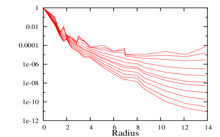
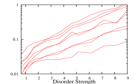
Figure 1: The left graph shows the normalized density matrix magnitude at ${\mu}=0$. Each line corresponds to a different disorder strength between $0.65$ and $9.00$; lower disorders are higher on the graph. The right graph shows the ratio of the square root of the second moment to the mean at $\mu=0$. The different lines correspond to different radii $r=n\sqrt{3}$, with smaller radii lower on the graph.

The left graph of figure 1 shows the normalized density matrix magnitude ${\frac{MDP{(\rho,\rho,r)}}{MDP{(\rho,\rho,0)}}}$ at ${\mu}=0$. For $r>0$ and $\sigma\geq 1.65$ a good fit to this quantity can be obtained by ${r^{-4}\exp{(\frac{-2r}{\tilde{R}})}}$, where the coherence length is given by $\tilde{R}={{({0.057\sigma}-{0.089}-{0.064{\sigma}^{-1}})}^{-1}}$. Note the almost inverse relation between the coherence length $\tilde{R}$ and the disorder strength $\sigma$. Lattice effects cause a systematic uncertainty in the first constant $0.057$ of roughly $30\%$. Similar fits can be obtained at other Fermi levels within the band ${|\mu|}\leq{6}$; the first constant has a minimum at $\mu=0$ and a total variation of about $30\%$.

Now I consider the statistical distribution of the density matrix magnitude. The right graph of figure 1 shows the ratio of the square root of the second moment to the mean. Note that this ratio seems to grow roughly exponentially with the disorder $\sigma$. An examination of the kurtosis (the normalized fourth moment of the statistical distribution) of the density matrix magnitude shows that for $\sigma\geq{5.15}$ this quantity becomes very large, starting at larger radii and larger Fermi level $|\mu|$. These statistics suggest that at the Anderson transition the statistical distribution of the density matrix magnitude develops a long tail; it loses its self-averaging property.

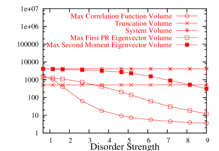
Figure 2: Important volume scales. Each volume measure was averaged across the ensemble and across a small interval of the energy spectrum. Shown here are the maximum values of these averages.

Figure 2 shows two measures of eigenvector volume. The first is the inverse of the first participation ratio; i.e. ${({\sum_{\vec{x}}{{|{\langle\psi|\vec{x}\rangle}|}^{2}}})}^{2}/{\sum_{\vec{x}}{{|{\langle\psi|\vec{x}\rangle}|}^{4}}}$. This quantity is a lattice friendly measure of volume because it has a minimum value of one when ${\langle\psi|\vec{x}\rangle}$ is a delta function and a maximum value of the system size when ${\langle\psi|\vec{x}\rangle}$ is a constant. Figure 2 shows that this volume becomes smaller than the truncation volume in the range $\sigma={3.00}$ to $\sigma={4.00}$.

My second volume measure is based on the second moment: ${({(2\pi)}^{D}{{det}{Q}})}^{\frac{-1}{2}}$ , where $Q$ is the second moment (or quadrupole tensor) of ${{|{\langle\psi|\vec{x}\rangle}|}^{2}}$. Unlike the first volume measure, this measure remains large even at large disorders, indicating that each eigenfunction consists of several isolated peaks scattered throughout the system volume. This structure is caused by the fact that states with similar energies will mix even if they are connected by exponentially small matrix elements. However, mixing caused by such small matrix elements does not influence the density matrix, because it essentially just induces a unitary transformation of the mixed eigenvectors, and as we know the density matrix is invariant under unitary transformations between states that are all either less than $\mu$ or more than $\mu$.

Figure 2 also shows the maximum value of the coherence volume; $V_{C}={{max}_{E}{V{(E)}}}$, where $V{(E)}$ is the coherence volume. I calculated this volume by first computing the correlation function ${C{(\vec{x})}}={\int{{d\vec{k}}^{D}{{|{\langle\vec{k}|\psi\rangle}|}^{2}{exp{(\imath{\vec{k}\cdot\vec{x}})}}}}}$, and then applying my two volume measures to ${C^{2}{(\vec{x})}}$. Taking the maximum value resolves an important ambiguity: at disorder strengths $\sigma\leq{6.15}$ the coherence length shows two peaks at energies ${|E|}={6-8}$. These peaks become very pronounced at $\sigma\leq 1.65$, where they are a factor of $10$ above the minimum. Note that the coherence volume becomes small much sooner than the eigenvector volume, in the range from $\sigma={1.65}$ to $\sigma={2.65}$. For $\sigma\geq{1.15}$ and $V_{C}\gg 1$ it is roughly proportional to ${{\sigma}^{-3}}$. This fits well with the density matrix’s coherence length at large $\sigma$, but not at small $\sigma$.

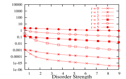
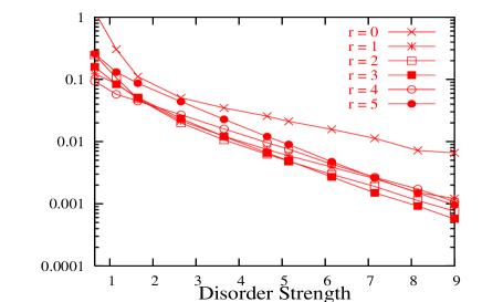
Figure 3: Relative error $e{(r,R)}$ (eq. 1) and absolute error error $E{(r,R)}$ (eq. 2) as a function of disorder. ${\mu}={0}$.

Figure 3 shows the relative error and absolute error as a function of disorder. The $O{(N)}$ algorithm begins to work well at $r={0,1}$ at quite small disorders, and the $r=2$ relative error falls to $1\%$ at about $\sigma\thickapprox{3}$. Clearly the $O{(N)}$ algorithm’s success is controlled by the coherence volume, not by the eigenvector volumes.

The overlapping lines in the right hand graph of figure 3 confirm section 5.2’s argument that the absolute error $E{(r,R)}$ is roughly independent of $r$, except at $r=0$. The magnification at $r=0$ is probably caused by the density matrix’s close relationship to the identity matrix. It is more than compensated for by a corresponding magnification of the density matrix at $r=0$, so that the left hand graph shows that the value of the relative error $e{(r,R)}$ at $r=0$ is smaller than its value at $r=1$.

Section 5.3 suggested that a small coherence length may cause a decrease in the absolute error $E{(r,R)}$ of order $\frac{{\eta}^{4}}{R^{4}}$. The $R=5$ line in the left hand graph of figure 3 shows that the decrease is actually even more pronounced: at the boundary $r=R$, $E{(r,R)}$ is of the same order of magnitude as $MDP{(f,f,r)}$, which is controlled by an exponential. This is just the ansatz used to obtain Eq. 3; my results fully support the validity of Eq. 3 except - as discussed before - at $r=0$, and at the edges of the energy band. Therefore accurate estimates of the error of an $O{(N)}$ calculation may be obtained from the results of the $O{(N)}$ calculation itself.

Section 5.1 showed that for large $R$ the absolute error $E{(r,R)}$ is bounded by a polynomial times $\exp{(-\frac{{4R}-{2r}}{L})}$, where $L$ is the decay length. This suggests an $r$ dependence which is not confirmed by the right hand graph of figure 3, where it would cause a splitting of the lines at $\sigma>{6.15}$. However, the previous paragraph showed that $E{(r,R)}$ actually depends on $R$ as $R^{-4}exp{(\frac{-2R}{\tilde{R}})}$, where $\tilde{R}$ is the coherence length. Therefore as long as ${\tilde{R}}<{2L}$, the bound obtained in section 5.1 is automatically verified at all $r$. Moreover at small $R$ the unknown polynomial in the bound may mask any $r$ dependence.

7 Reliability of These Results

I have already discussed the errors due to the finite lattice size and to the truncation of the Cheybyshev expansion. While a precise analytical and numerical treatment of both error sources is possible, my checks indicate that they will have at most a quantitative, not qualitative, effect on the results of this paper. The main risks to the results probably lie in two areas: finite ensemble size, and software reliability and reproducibility. I have taken steps to manage both issues:

7.1 Finite ensemble size.

All results presented here were obtained from ensembles of $33$ realizations, but repeating the calculations with ensembles of $100$ realizations yielded the same results. At the critical disorder the same quantities were computed with three different lattice sizes ($100$ realizations at both ${12}^{3}$ and ${16}^{3}$, and $10$ realizations at ${20}^{3}$), and the agreement is very good. Graphing any quantity across several disorders, one immediately notices that there is little noise induced overlap of the two graphs. Therefore, it seems likely that risks due to finite ensemble size are under control.

7.2 Software Reliability and Reproducibility.

I have tried very hard to reduce this risk. The software includes an automated test suite which tests all computational functions except the highest level output (graph printing) routines. Moreover, I have taken pains to enable other researchers to easily reproduce and check my results, simply by installing my software and the libraries it depends on, compiling it with the GNU gcc compiler[27], and starting it running. The software, with all needed configuration files, is available under the GNU Public License[26]; check www.sacksteder.com for further details.

Special thanks to my advisor, Giorgio Parisi, for his attentiveness, stimulation, and encouragement. Thank you also to Stephan Goedecker for sharing one of his $O{(N)}$ codes, to the OXON group for sharing their code (though it remained unused), and to the organizers of the 21st International Workshop on Numerical Linear Algebra and its Applications for putting that event together.

References

- [1] Ordejon P. Order-N tight-binding methods for electronic structure and molecular dynamics. Computational Materials Science 1998; 12:157–191.
- [2] Scuseria GE. Linear scaling density functional calculations with gaussian orbitals. Journal of Physical Chemistry A 1999; 103(25):4782–4290.
- [3] Abrikosov IA, Niklasson AMN, Simak SI, Johansson B, Ruban AV, Skriver HL. Order-N Green’s function technique for local environment effects in alloys. Physical Review Letters 1996; 76(12):4203–4206.
- [4] Abrikosov IA, Simak SI, Johansson B, Ruban AV, Skriver HL. Locally self-consistent Green’s function approach to the electronic structure problem. Physical Review B 1997; 56(15):9319–9334.
- [5] Economou EN, Soukoulis CM, Zdetsis AD. Loocalized states in disordered systems as bound states in potential wells. Physical Review B 1984; 360(4):1686–1694.
- [6] Baer R, Head-Gordon M. Sparsity of the density matrix in Kohn-Sham density functional theory and an assessment of linear system-size scaling methods. Physical Review Letters 1997; 79(20):3962–3965.
- [7] Baer R, Head-Gordon M. Chebyshev expansion methods for electronic structure calculations on large molecular systems. Journal of Chemical Physics 1997; 107(23):10003–10013.
- [8] Goedecker S. Decay properties of the finite-temperature density matrix in metals. Physical Review B 1998; 58(7):3501–3502. arXiv:cond-mat/9804013.
- [9] Ismail-Beigi S, Arias T. Locality of the density matrix in metals, semiconductors, and insulators. Physical Review Letters 1999; 82(10):2127–2130.
- [10] Goedecker S, Ivanov OV. Frequency localization properties of the density matrix and its resulting hypersparsity in a wavelet representation. Physical Review B 1999; 59(11):7270–7273.
- [11] Goedecker S. Linear scaling electronic structure methods. Reviews of Modern Physics 1999; 71(4):1085–1123.
- [12] Zhang X, Drabold DA. Properties of the density matrix from realistic calculations. Physical Review B 2001; 63(23):233109–233112.
- [13] Koch E, Goedecker S. Locality properties and Wannier functions for interacting systems. Solid State Communications 2001; 119:105–109. arXiv:cond-mat/0105401.
- [14] He L, Vanderbilt D. Exponential decay properties of Wannier functions and related quantities. Physical Reviw Letters 2001; 86(23):5341–5344. arXiv:cond-mat/0102016.
- [15] Taraskin SN, Fry PA, Zhang X, Drabold DA, Elliott SR. Spatial decay of the single-particle density matrix in tight-binding models: analytic results in two dimensions. Physical Review B 2002; 66(23):233101–233104.
- [16] Slevin K, Ohtsuki T. Numerical verification of universality for the Anderson transition. Physical Review B 2001; 63(4):45108-45112. arXiv:cond-mat/0101272.
- [17] Kantelhardt JW, Bunde A. Sublocalization, superlocalization, and violation of standard single-parameter scaling in the Anderson model. Physical Review B 2002; 66(3):35118–35128. arXiv:cond-mat/0201356.
- [18] Anderson PW. Absence of diffusion in certain random lattices. Physical Review 1958; 109(5):1492–1505.
- [19] Bulka B, Schreiber M, Kramer B. Localization, quantum interference, and the metal-insulator transition. Zeitschrift fur Physik B: Condensed Matter 1987; 66:21–30.
- [20] Resta R. Why are insulators insulating and metals conducting? Journal of Physics: Condensed Matter 2002; 14:R625–R626.
- [21] Yang W. Direct calculation of electron density in density-functional theory. Physical Review Letters 1991; 66(11):1438–1441.
- [22] Goedecker S, Colombo L. Efficient linear scaling algorithm for tight-binding molecular dynamics. Physical Review Letters 1994; 73(1):122–125.
- [23] Goedecker S, Teter M. Tight-binding electronic structure calculations and tight-binding molecular dynamics with localized orbitals. Physical Review B 1995; 51(15):9455–9464.
- [24] Bowler DR, Gillan MJ. Density matrices in O(N) electronic structure calculations: theory and applications. Computer Physics Communications 1999; 120(2-3):95–108. arXiv:cond-mat/9810042.
-
[25]
Schubert G, Weisse A, Fehske H.
Comparative numerical study of localization in disordered electron systems.
http://arxiv.org 2003; arXiv:cond-mat/0309015. [28 November 2003]. -
[26]
Licenses.
http://www.gnu.org/licenses/licenses.html [28 November 2003]. -
[27]
Welcome to the GCC home page!
http://www.gnu.org/software/gcc/gcc.html [28 November 2003].