Full Counting Statistics of Spin Currents

Abstract

We discuss how to detect fluctuating spin currents and derive full counting statistics of electron spin transfers. It is interesting to consider several detectors in series that simultaneously monitor different components of the spins transferred. We have found that in general the statistics of the measurement outcomes cannot be explained with the projection postulate and essentially depends on the quantum dynamics of the detectors.

The detection and statistics of quantum fluctuations attracts increasingly the attention of the physical community. The Full Counting Statistics (FCS) Levitov and Lesovik (1993); Levitov et al. (1996) of quantum electron transport provides all possible information about fluctuations of electric current in mesoscopic systems. The FCS has been evaluated for charge transport between superconducting Belzig and Nazarov (2001) and superconducting-normal leads Belzig (2002) by nonequilibrium Green function method Nazarov (1999). An approach to FCS of a general variable presented in Kindermann and Nazarov (2002) allows one to resolve possible inconsistencies that concern the quantum measurement problem by explicitly incorporating the dynamics of a detector.

There is a strong current interest to new ways to manipulate, control and measure electron spins in solid state. This defines the field of spintronics Awschalom et al. (2002) that aims to gain the same control over spin as one currently has over charge. This provides a motivation to study the FCS of spin current. This statistics is of fundamental interest since different components of spin do not commute, this makes the problem of corresponding quantum measurement especially relevant.

In this Letter, we propose a realization of a spin current detector. We derive the FCS of a spin current, originating from a flow of unpolarized particles, that is measured by such detector(s). We focus on the cases where two and three components of the spin current are detected simultaneously by two or three detectors in series. Naïvely, one could try to describe the FCS of such a combined measurement by applying the Projection Postulate after the measurement by each detector. We explicitly demonstrate that for the case of three detectors the FCS cannot be explained in such a straightforward way and depends on quantum dynamics of the central detector.

We consider two-terminal electric circuit where electrons are transferred between the terminals through a contact. The theory of FCS is elaborated in detail for the case when this contact can be described in the Landauer-Büttiker scattering framework. In fact, our results do not depend on the type of the contact provided it does not polarize the spin of electrons transferred, nor such polarization occurs in the terminals. Thus, all of our results can be applied as well to neutron sources. Since the electrons carry spin, the charge transfer between the terminals should be accompanied by spin transfer although there is no average spin current between the terminals. Therefore, there are fluctuations of spin current. How to measure them?

This can be probably done in many ways, for instance, by exploiting the spin-valve effect Tsymbal and Pettifor (2001). In the present Letter, we concentrate on a different setup proposed and used in Cimmino (1989) to detect Aharonov-Casher effect Aharonov and Casher (1984) for neutrons. This setup exploits the fact that a moving magnetic dipole generates an electric one Costa de Beauregard (1967). To measure this, one encloses the two-dimensional current lead between the plates of a capacitor as shown in Fig. 1. Each spin moving with velocity $\mathbf{v}$ produces a dipole moment $\mathbf{d}=\frac{g}{2}\mu_{B}(\frac{\mathbf{v}}{c}\times\mathbf{S})$, $g$ being the gyromagnetic factor, $\mu_{B}$ Bohr’s magneton, $c$ the speed of light, and electron spin $\mathbf{S}$ is measured in units of $\hbar/2$. This moment induces a voltage drop $V$ between the plates, which is the detector read-out, the variable being measured. Since the interaction between the dipole moment and electric field $\mathbf{E}$ in the capacitor is $H_{int}=-\mathbf{E}\cdot\mathbf{d}$, the read-out signal is proportional to spin current in the lead $\mathbf{J}$, $V=\lambda\mathbf{n}\cdot\mathbf{J}$, $\mathbf{n}$ being the unit vector perpendicular to the direction of the current flow and parallel to the plates of the capacitor, $\lambda$ being a proportionality coefficient. The concrete expression for the latter, $\lambda=\frac{g}{2}\frac{L_{\shortparallel}}{w}\frac{\mu_{B}}{Cc}$, depends on the capacitance $C$ and geometrical dimensions: the length of its plates in the direction of the current $L_{\shortparallel}$, and the distance between the plates $w$.

The variable canonically conjugated to the read-out is the charge $Q$ in the capacitor, and the expression for the interaction in terms of $Q$ contains the same proportionality coefficient $\lambda$, $H_{int}=-\lambda Q\mathbf{n}\cdot\mathbf{J}$. Our choice of the detection setup is motivated by the fact that this detector does not disrupt electron transfers through the contact and only gives a minimal feedback: the electrons passing the capacitor in the direction of current acquire Aharonov-Casher phase shift. This phase shift depends on spin and is given by $\Phi_{AC}=\lambda Q\mathbf{n}\!\cdot\!\mathbf{S}/\hbar$. This is similar to the detection scheme presented in Levitov et al. (1996) for charges transferred. A fundamental complication in comparison with the charge FCS is that in our case the phase shift depends on spin, so that even the minimal feedback may cause the rotation of spin of the electron that passes the capacitor.

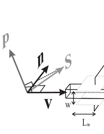
Figure 1: The proposed spin current detector. An electron with velocity $\mathbf{v}$ and spin $\mathbf{S}$ induces a voltage drop in a capacitor. The electric field $\mathbf{E}$ inside the capacitor produces an Aharonov-Casher phase shift on the electrons.

It is important to require that charge and spin current are the same in the contact and in the detector. To assure that spin current conserves, neither the length of the detector $L_{\shortparallel}$ nor the distance from detector to contact should exceed the spin relaxation length. In addition to this, there should be no spin or charge accumulation between the contact and the detector. This is always true for low-frequency fluctuations of charge or spin current.

We will see that the most interesting setup includes several detectors in series as presented in Fig. 2. It may also include a charge detector. The spin detectors can have arbitrary polarization vectors $\mathbf{n}_{a}$. This can be achieved by turning the current lead and the capacitor plates in different directions. The contact is biased by a voltage source $V_{ext}$. Since we assume that the resistance brought by detectors is much smaller than that of the contact, the whole voltage drops at the contact and the contact works as a fluctuating source of (spin) current measured by (spin) detectors.

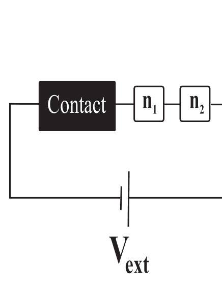
Figure 2: The setup considered, in the case of three spin detectors and one charge detector.

Let us compare the detection scheme proposed with the one used in Stern-Gerlach experiment Gerlach and Stern (1922). In this classical experiment, an unpolarized beam of spin $1/2$ atoms was split into two sub-beams corresponding to two different projections of spin onto an axis set by magnetic field. The intensities of the beams are then detected, and at this stage the wave function collapse is said to happen: the spin projection of each atom detected is with certainty $\pm\hbar/2$ depending on the beam. If one would force these atoms to pass the subsequent Stern-Gerlach detectors, the readings of these detectors can be predicted from this fact.

In our detection scheme, a single detector does the same as a Stern-Gerlach one: it measures the difference of numbers of particles passed with spin “up” and “down” with respect to the polarization vector $\mathbf{n}$. What can we say about the readings of subsequent detectors? A straightforward assumption would be that the second detector, like in Stern-Gerlach experiment, measures the statistical mixture of the states with the certain projection on the polarization vector of the first detector (the wave function is ”collapsed” after the first measurement). We will refer to this assumption as to Projection Postulate (PP).

We will explicitly show that it is not what happens in our detection scheme if there are at least three detectors: the FCS of readings differs form the one predicted with using PP. The difference shows up in second and fourth order cumulants of spin currents, and the fact that the wave function is not collapsed can be just simply observed in this way.

We adopt the fully quantum definition of FCS that has been put forward in Kindermann and Nazarov (2002). We consider a number of spin current detectors in series, labelled by index $a$ that increases from the contact to the terminal (Fig. 2), next to a charge detector (ammeter). We consider the couplings between the detector degrees of freedom and the system, $\hat{H}_{int}=-\frac{\hbar}{e}\hat{\chi}\hat{I}-\sum_{a}\hbar\hat{\gamma}_{a}\mathbf{n}_{a}\!\cdot\!\mathbf{\hat{J}}$. Here $\hat{\gamma}_{a}\equiv\lambda_{a}\hat{Q}_{a}/\hbar$ are proportional to operators of charge in the capacitors of the corresponding spin current detectors, and $\hat{\chi}$ is the degree of freedom of the charge detector. The FCS is defined as a kernel that relates the initial density matrix of all detectors to the final one, that one after the measurement,

$$\rho_{f}(\chi^{+},\gamma^{+}_{a};\chi^{-},\gamma_{a}^{-})=$$

$$e^{-\tau F(\chi^{+}-\chi^{-},\gamma^{+}_{a},\gamma^{+}_{a})} \rho_{in}(\chi^{+},\gamma^{+}_{a};\chi^{-},\gamma^{-}_{a})$$ (1)

The most general result we report here is that this FCS can be directly expressed in terms of charge counting statistics $F_{c}$, provided neither the contact nor the terminals polarize the electrons transferred. In this case,

$$F(\chi,\{\gamma^{+}_{a}\},\{\gamma^{-}_{a}\})=\frac{1}{2}\sum_{\pm}F_{c}(\chi\pm\alpha)$$ (2)

where $e^{\pm i\alpha}$ are the eigenvalues of the $2\times 2$ matrix

$$\prod^{\rightarrow}_{a}e^{i\gamma^{+}_{a}\mathbf{n}_{a}\cdot\boldsymbol{\sigma}}\prod^{\leftarrow}_{a}e^{-i\gamma^{-}_{a}\mathbf{n}_{a}\cdot\boldsymbol{\sigma}}\;.$$ (3)

In this matrix, $\boldsymbol{\sigma}$ is a pseudovector of $2\times 2$ Pauli matrices, and $\prod\limits^{\rightarrow}_{a}(\prod\limits^{\leftarrow}_{a})$ denotes the product ordered with decreasing (increasing) $a$.

We arrive to the relation (2) by extending the scattering theory of FCS. By virtue of (spin) current conservation, the coupling terms $\hat{H}_{int}$ can be gauged away and ascribed to the electron Green functions of the terminal Levitov et al. (1996); Belzig and Nazarov (2001). While for charge counting statistics this gauge transform is just a multiplication by a phase factor $e^{i\chi}$ the gauge transform generated by a spin detector $a$ involves a unitary matrix in spin space, $e^{i\gamma_{a}\mathbf{n}_{a}\cdot\mathbf{\sigma}}$. The total transform is thus the product of these matrices nested in a proper order. We notice that for the unpolarizing circuit this transform just commutes with the Hamiltonian. This enables one to derive the relation (2).

For the case of one or two detectors in series, the eigenvalues $e^{\pm i\alpha}$ are not affected by the order of matrix multiplication in (3) and depend on differences of spin counting fields $\gamma_{a}\equiv\gamma^{+}_{a}-\gamma^{-}_{a}$ only. This implies that the FCS definition (1) can be readily interpreted in classical terms: it is a generating function for probability distribution of a certain number of spin counts $S_{a}$ in each detector,

$$P(\{S_{a}\})=\int\prod_{a}d\gamma_{a}e^{-\tau F(0,\{\gamma_{a}\})}e^{-i\sum_{a}S_{a}\gamma_{a}}$$ (4)

For a single detector, the spin FCS is very simple: it corresponds to independent transfer of two sorts of electrons, with spins ”up” and ”down” with respect to quantization axis. The (higher-order) cumulants of the spin (charge) transferred are given by (higher-order) derivative of $F$ with respect to $\gamma_{a}$($\chi$), at $\chi=\gamma_{a}=0$. From this and relation (2) we conclude that all odd cumulants of spin current are 0 while all even cumulants equal to even cumulants of the charge transferred.

It is interesting to note that in the case considered one can provide a ”reasonable alternative” to the consistent quantum mechanical derivation. One can evaluate FCS assuming that the probability to measure a certain spin count in the detector $m$ only depends on the count of the immediately preceding detector $m-1$. This corresponds to the PP: after each measurement, the wave function collapses to one of the eigenstates loosing memory about the previous evolution. We calculate conditional probability for two detectors and then nest these probabilities to obtain that the probability distribution for spin counts is given by Eq. (4), with $F$ determined by Eq. (2) with a different parameter $\alpha$, given by

$$\cos{\alpha_{\raisebox{-1.0pt}{${}_{PP}$}}}\!\!=\!\!\sum_{\mu_{a}=\pm 1}e^{i\!\sum_{a}\!\mu_{a}\gamma_{a}}\frac{1}{2}\!\prod_{a=1}^{K-1}\frac{1\!+\!\mu_{a}\mu_{a+1}\mathbf{n}_{a}\!\cdot\!\mathbf{n}_{a+1}}{2}.$$ (5)

We note that $\alpha_{PP}$ depends only on the differences $\gamma_{a}=\gamma_{a}^{+}-\gamma_{a}^{-}$. Eq. (5) facilitates the comparison of the results of two approaches and allows us to pinpoint the quantum mechanical features missed in PP analysis.

We stress that for the case of one or two spin detectors, $\alpha=\alpha_{PP}$, and the approaches give precisely the same result. Essentially, the result for two detectors can be understood in terms of the probability to have the same or opposite spin counts for one electron that passes both detectors. The probability of having the same counts is simply $P_{12}=(1+\mathbf{n}_{1}\!\cdot\!\mathbf{n}_{2})/{2}$. For second order cumulants — noises — one obtains $\langle\!\langle S^{2}_{1}\rangle\!\rangle=\langle\!\langle S^{2}_{2}\rangle\!\rangle=\langle\!\langle N^{2}\rangle\!\rangle$, $\langle\!\langle S_{1}S_{2}\rangle\!\rangle=\mathbf{n}_{1}\!\cdot\!\mathbf{n}_{2}\langle\!\langle N^{2}\rangle\!\rangle$, $\langle\!\langle N^{2}\rangle\!\rangle$ being the charge noise, i.e. the second cumulant of the number of transferred particles. The detector feedback is irrelevant, so it is possible to measure two spin components within the setup studied.

Let us now consider three spin detectors with arbitrary $\mathbf{n}_{1,2,3}.$ In this case, the FCS defined by Eq. (2) cannot be immediately interpreted in terms of probability distribution Eq. (4). To illustrate this explicitly, let us consider the change of density matrix upon one electron passing all detectors. In $\gamma_{a}$-representation it is given by $\rho_{f}(\gamma^{+}_{a};\gamma_{a}^{-})=\cos{\alpha}~{}\rho_{in}(\gamma^{+}_{a};\gamma^{-}_{a})$, where $\alpha$ in the case of three detectors assumes the following form:

$$\cos\alpha=\cos{\alpha_{PP}}-\sin{\gamma}_{3}\sin{\gamma}_{1}\left[\right.$$

$$\left.\cos\Gamma_{2}\left({\mathbf{n}}_{1}\!\cdot\!{\mathbf{n}}_{3}-({\mathbf{n}}_{1}\!\cdot\!{\mathbf{n}}_{2})({\mathbf{n}}_{2}\!\cdot\!{\mathbf{n}}_{3})\right)\!+\!\sin{\Gamma_{2}}({\mathbf{n}}_{1}\times{\mathbf{n}}_{2})\!\cdot\!{\mathbf{n}}_{3}\right],$$

$$\cos\alpha_{PP}=\cos{\gamma}_{1}\cos{\gamma}_{2}\cos{\gamma}_{3}$$

$$-\sin{\gamma}_{1}\sin{\gamma}_{2}\cos{\gamma}_{3}{\mathbf{n}}_{1}\!\cdot\!{\mathbf{n}}_{2}-\sin{\gamma}_{2}\sin{\gamma}_{3}\cos{\gamma}_{1}{\mathbf{n}}_{2}\!\cdot\!{\mathbf{n}}_{3}+$$

$$-\sin{\gamma}_{3}\sin{\gamma}_{1}\cos{\gamma}_{2}({\mathbf{n}}_{1}\!\cdot\!{\mathbf{n}}_{2})({\mathbf{n}}_{2}\!\cdot\!{\mathbf{n}}_{3}).$$ (6)

where $\Gamma_{2}\equiv\gamma^{+}_{2}+\gamma^{-}_{2}$. Thus the multiplication with $\cos\alpha$ corresponds to multiplication with several $\exp(\pm i\gamma)$, $\exp(\pm i\Gamma_{2})$ and adding the results with some weights. Let us assume that initial density matrix corresponds to the state with certain number of counts in each detector. Since the “number of counts” representation is obtained from the $\gamma_{a}$-representation by Fourier transforming with respect to $\gamma^{\pm}_{a}$, multiplication with $\exp(\pm i\gamma_{a})$ transforms diagonal elements of density matrix into diagonal ones; $\rho(S_{a},S_{a})\rightarrow\rho(S_{a}\pm 1,S_{a}\pm 1)$, and the state with a well-defined number of counts remains such. However, the multiplication with $\exp(\pm i\Gamma_{2})$ produces non-diagonal elements from diagonal ones; $\rho(S_{2},S_{2})\rightarrow\rho(S_{2}\pm 1,S_{2}\mp 1)$. One readily sees from Eq. (6) that this is disregarded if one applies PP. This seems OK since non-diagonal elements do not contribute to probabilities. However, if another electron passes the second detector, the non-diagonal elements can be again transformed into diagonal ones and do contribute to the probability distribution of the counts. Thus, the second detector disturbs the correlation of read-outs in the first and third detector. The actual FCS will depend on the dynamics of the second detector since its feedback is unavoidable. This feedback is eventually an Aharonov-Casher effect: the electrons passing the second detector acquire phase shift $\pm\Gamma_{2}$, this corresponds to rotation of their spin by angle $\Gamma_{2}$ about the axis $\mathbf{n}_{2}$. Theoretically, one could prepare the second detector in a given state and then observe the dependence of FCS on this state. However, in the present Letter we would like to describe a more realistic situation where no special preparation takes place and the degree of freedom of the second detector just fluctuates following its own (dissipative) dynamics. We illustrate the effect with a simple model of such dynamics: $\Gamma_{2}$ exhibits time-dependent Gaussian fluctuations described by the following action

$${\mathcal{S}}_{det}=\frac{1}{2}\int dt\left((\dot{\Gamma}_{2}(t))^{2}\tau_{c}+\frac{(\Gamma_{2}(t)-\Gamma_{0})^{2}}{4\tau_{c}\langle\!\langle\Gamma^{2}\rangle\!\rangle^{2}}\right)$$ (7)

so that it fluctuates around the averaged value $\Gamma_{0}$ with the variance $\langle\!\langle\Gamma^{2}\rangle\!\rangle$ and typical correlation time $\tau_{c}\langle\!\langle\Gamma^{2}\rangle\!\rangle$. The generating function of the actual FCS results from the averaging of the Eq. (2) over fluctuations of $\Gamma_{2}$,

$${\mathcal{Z}}(\{\gamma_{a}\})=\int{\mathcal{D}}\Gamma(t)e^{-{\mathcal{S}}_{det}-\int_{0}^{\tau}\!F(\alpha(\{\gamma_{a}\},\;\Gamma_{2}(t)))dt}$$ (8)

This allows us to compute the cumulants of spin counts and compare them with PP expressions given by Eqs. (4), (6). The difference is in principle noticeable for the second order cumulants — noise correlations in the first and in the third detectors,

$$\langle\!\langle S_{1}S_{3}\rangle\!\rangle\!=\!\langle\!\langle N^{2}\rangle\!\rangle\left[C+\left(\tilde{\mathbf{n}}_{1}\cdot\mathbf{n}_{3}-C\right)e^{-\langle\!\langle\Gamma^{2}\rangle\!\rangle/2}\right],$$ (9)

where $C\equiv(\mathbf{n}_{1}\cdot\mathbf{n}_{2})(\mathbf{n}_{2}\cdot\mathbf{n}_{3})$, $\tilde{\mathbf{n}}_{1}$ is the vector $\mathbf{n}_{1}$ rotated about $\mathbf{n}_{2}$ by the angle $\Gamma_{0}$, and the first term presents the PP result.

The second term, as expected, has a typical signature of interference effects: it is suppressed exponentially if the variance of the corresponding Aharonov-Casher phase $\langle\!\langle\Gamma^{2}\rangle\!\rangle\gg 1$. Since $\Phi_{AC}$ is inversely proportional to $\hbar$, this is the classical limit. In this limit, the result coincides with the PP.

However, if one goes to fourth order cumulants — correlations of noises — one observes big deviations from PP even in the classical limit. We obtain that

$$\langle\!\langle S_{1}^{2}S_{3}^{2}\rangle\!\rangle \!=\!\langle\!\langle S_{1}^{2}S_{3}^{2}\rangle\!\rangle_{\raisebox{-2.84526pt}{${}_{\!\!PP}$}}+$$ (10)

$$+\frac{2}{3}A\left[\langle\!\langle N^{4}\rangle\!\rangle-\langle\!\langle N^{2}\rangle\!\rangle\right]+16\frac{\tau_{c}}{\tau}A\langle\!\langle N^{2}\rangle\!\rangle^{2},$$

where $A\equiv\left[1-(\mathbf{n}_{1}\!\cdot\!\mathbf{n}_{2})^{2}\right]\left[1-(\mathbf{n}_{2}\!\cdot\!\mathbf{n}_{3})^{2}\right]$, and the PP result is expressed in terms of charge cumulants as

$$\langle\!\langle S_{1}^{2}S_{3}^{2}\rangle\!\rangle_{\raisebox{-2.84526pt}{${}_{\!PP}$}}\!\!=(1+2C^{2})\langle\!\langle N^{4}\rangle\!\rangle+2(1-C^{2})\langle\!\langle N^{2}\rangle\!\rangle.$$

This deviation results from correlations of $\Gamma_{2}$ at time scale $\tau_{c}$. To estimate the result, we notice that the charge cumulants are of the order of $\tau/\tau_{el}$, $\tau_{el}$ being the average time between electron transfers. It is easy to fulfill the condition $\tau_{el}\ll\tau_{c}\ll\tau$, and in this case $\langle\!\langle S_{1}^{2}S_{3}^{2}\rangle\!\rangle$ is much bigger than PP result.

In conclusion, we have discussed the full counting statistics of spin currents measured by the detectors that provide the minimum back-action to the passing particles. This FCS can be evaluated quite generally for unpolarized currents. We compare the actual FCS with the predictions of Projection Postulate and find an agreement for one and two detectors. However, the FCS of three detectors in series displays both explicit dependence on dynamics of the second detector and significant deviations from PP predictions. These deviations can be observed in second and fourth order cumulants of spin currents.

We acknowledge the financial support provided through the European Community’s Research Training Networks Programme under contract HPRN-CT-2002-00302, Spintronics. We are grateful to R. Fazio and A. Romito for interesting discussions.

References

- Levitov and Lesovik (1993) L. S. Levitov and G. B. Lesovik, JETP Lett. 58, 230 (1993).
- Levitov et al. (1996) L. S. Levitov, H. W. Lee, and G. B. Lesovik, Journ. Math. Phys. 37, 4845 (1996).
- Belzig and Nazarov (2001) W. Belzig and Yu. V. Nazarov, Phys. Rev. Lett. 87, 197006 (2001).
- Belzig (2002) W. Belzig, in Quantum Noise in Mesoscopic Physics, edited by Yu. V. Nazarov (Kluwer, 2002).
- Nazarov (1999) Yu. V. Nazarov, Ann. Phys. (Leipzig) SI-193, 507 (1999).
- Kindermann and Nazarov (2002) M. Kindermann and Yu. V. Nazarov, in Quantum Noise in Mesoscopic Physics, edited by Yu. V. Nazarov (Kluwer, 2002); idem, cond-mat/0107133.
- Awschalom et al. (2002) D. D. Awschalom, D. Loss, and N. Samarth, eds., Semiconductor Spintronics and Quantum Computation (Springer, 2002).
- Tsymbal and Pettifor (2001) E. Y. Tsymbal and D. G. Pettifor, in Solid State Physics, edited by H. Ehrenreich and F. Spaepen (Academic Press, 2001), vol. 56.
- Cimmino (1989) A. Cimmino et al., Phys. Rev. Lett. 63, 380 (1989).
- Aharonov and Casher (1984) Y. Aharonov and A. Casher, Phys. Rev. Lett. 53, 319 (1984).
- Costa de Beauregard (1967) O. Costa de Beauregard, Phys. Lett. A 24, 177 (1967).
- Gerlach and Stern (1922) W. Gerlach and O. Stern, Z. Phys. 9, 349 (1922).