Community analysis in social networks

Abstract

We present an empirical study of different social networks obtained from digital repositories. Our analysis reveals the community structure and provides a useful visualising technique. We investigate the scaling properties of the community size distribution, and that find all the networks exhibit power law scaling in the community size distributions with exponent either $-0.5$ or $-1$. Finally we find that the networks’ community structure is topologically self-similar using the Horton-Strahler index.

1 Introduction

The topology of complex networks have been the subject of intensive study over the past few years. It has been recognised that such topologies play an extremely important role in many systems and processes, for example, flow of data in computer networks Menezer03 , energy flow in food webs Garlasch03 , diffusion of information in social networks newman_rev , etc. This has led to advances in fields as diverse as computer science, biology and social science to name but a few.

It has recently been found that social networks exhibit a very clear community structure. For example, in an organisation, such community structure corresponds, to some extent, to the formal chart, and to some extend to ties between individuals arising due to personal, political and cultural reasons, giving rise to informal communities and to an informal community structure. The understanding of informal networks underlying the formal chart and of how they operate are key elements for successful management. In other scenarios, this community structure reflects in general the self-organisation of individuals to optimise some task performance, for example, optimal communication pathways or even maximisation of productivity in collaborations. Characterising and understanding this structure may be fundamental to the study of dynamical processes that occur on these nets. In this paper we present the empirical study of several social networks at the level of community structure. We show that all exhibit self-similar properties, with the community size distributions following power laws. The exponents of these power laws seem to fall into two distinct classes, one with exponent $\sim-0.5$ and the other with exponent $\sim-1$. The source of these two different scaling laws is still being investigated.

In the next section we describe the methodology used to characterise the social structure of the networks we study. In Section 3, we apply this methodology to various networks, and in Section 4 we characterise the community structure. Finally we present an interpretation of the results and propose some future work.

2 The method

2.1 Identification of real communities

The traditional method for identifying communities in networks is hierarchical clustering jain88 . Given a set of N nodes to be clustered, and an N$\times$N distance (or similarity) matrix, the basic process of hierarchical clustering is this: Start by assigning each node its own cluster, so that if you have N nodes, you now have N clusters, each containing just one node. Let the distances between the clusters equal the distances between the nodes they contain. Find the closest (or most similar) pair of clusters and merge them into a single cluster, so that now you have one less cluster. Compute distances between the new cluster and each of the old clusters. Repeat until all nodes are clustered into a single cluster of size N.

In this work we use a different community identification algorithm, proposed recently by Girvan and Newman (GN) girvan02 . This new algorithm gives successful results even for networks in which hierarchical clustering methods fail. The algorithm works as follows. The betweenness of an edge is defined as the number of minimum paths connecting pairs of nodes that go through that edge wasserman94 ; newman01 . The GN algorithm is based on the idea that the edges which connect highly clustered communities have a higher edge betweenness—for example edge $BE$ in Figure 1a—and therefore cutting these edges should separate communities. Thus, the algorithm proceeds by identifying and removing the link with the highest betweenness in the network. This process is repeated (should it be necessary) until the ‘parent network splits, producing two separate ‘offspring’ networks. The offspring can be split further in the same way until they contain only one node. In order to describe the entire splitting process, we generate a binary tree, in which bifurcations (white nodes in Figure 1b) depict communities and leaves (black nodes) represent individuals. All the information about the community structure of the original network can be deduced from the topology of the binary tree constructed in this fashion.

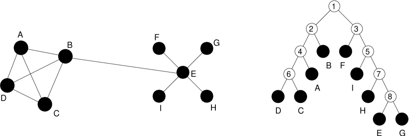
(a)                                                                  (b)

Figure 1: Community identification according to the GN algorithm. (a) A network containing two clearly defined communities connected by the link $BE$. This link will have the highest betweenness, since to get from any node in one community, to any node in the other, this link needs to be used. Therefore it will be the first link to be cut, splitting the network in two. The process of cutting this link corresponds to the bifurcation at the highest level of the binary tree in (b). Since there is no further community structure in the offspring networks, the rest of the nodes will be separated one by one, generating a binary tree with two branches corresponding to the two communities. For the community on the right, the most central node will be separated last. In general, branches of the binary tree correspond to communities of the original network and the tips of these branches correspond to the central nodes of the communities.

2.2 Graphical representation of the hierarchical community structure

Consider again the network in Figure 1a. At the beginning of the process, no links have been removed and the whole network is represented by node 1 in the binary tree of Figure 1b. When edge $BE$ is removed, the network splits in two groups: group 2, containing nodes $A$ to $D$, and group 3, containing nodes $E$ to $I$. After this first splitting, two completely separate communities are left, a very homogeneous one and a very centralised one. One can check that in both cases the algorithm will separate nodes one by one giving rise to two different branches in the binary tree. Actually, when communities with no further internal structure are found, they are disassembled in a very uneven way giving rise to branches. In other words, the almost impossible task of identifying communities from the original network is replaced by the easy task of identifying branches in the binary tree. When centralised network structures are treated, the central node(s) will appear at the end of the branch, thus also providing a method of identifying the “leaders” of each community.

3 Applications

In this section we apply the method described in the previous section to various networks. In Table 1 we present the characterising statistics of each of the networks.

Network	$N$	$\langle d\rangle$	$\langle C\rangle$
mail	1134	2.42	0.31
jazz	1265	2.79	0.89
fises	784	5.71	0.78
gr-qc	2546	6.11	0.54
hep-lat	1411	4.71	0.66
quant-ph	1460	5.97	0.71
math-ph	2117	10.13	0.58

Table 1: Statistics for the networks we study. $N$ is the number of nodes in the network,$\langle d\rangle$ is the average distance between nodes and $\langle C\rangle$ is the clustering coefficient. Note that the clustering coefficient all the networks apart from the mail network are extremely high. This is due to the networks’ construction as bipartite graphs. For example, in the ArXiv network, if four authors coauthor only one paper, the clustering coefficient of those four nodes in the network will be 1.

3.1 E-mail network

We extract and build a network of interactions via e-mail using logs from mail servers over a period of 3 months. In order to be able to concentrate on the real social structure, we remove ’spam’ mails with more than 50 recipients, and only create links between people that have exchanged e-mails, that is, an e-mail that was sent from A to B was responded to within the 3 month period. More information can be found in guimera??b .

Figure 2a shows the binary tree that results from the application of our method to the e-mail network of URV. Each colour corresponds to an individual’s affiliation to a specific centre within the university. Centres are in most of the cases faculties or colleges—for example the School of Engineering—and are usually comprised of departments—for example, the Department of Computer Sciences and Mathematics or the Electrical Engineering Department. In turn, departments are divided into research teams—for instance, the group of Complex Systems or the group of Dynamical Systems in the Department of Computer sciences and Mathematics.

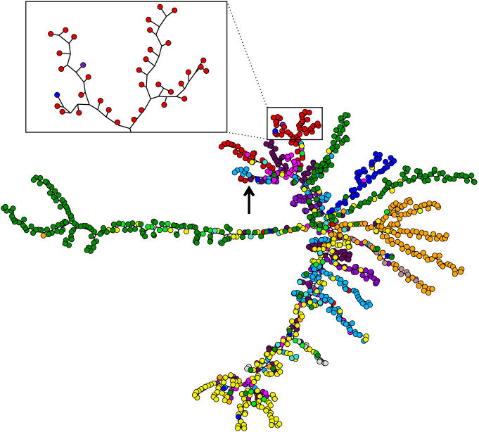
(a)

    

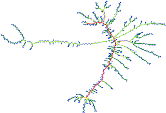
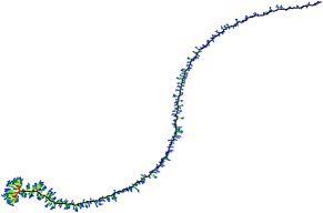
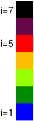
(b)                                       (c)

Figure 2: (a) Binary tree showing the result of applying the GN algorithm and our visualisation technique to the e-mail network of URV. Each branch corresponds to a real community and the tips of the branches correspond to their leaders. The splitting procedure starts in the position indicated by an arrow at the top of the drawing and proceeds downward. The colour of the nodes represents different centres within the university (five small centres containing less than 10 individuals are assigned the same colour). Nodes of the same colour (from the same centre) tend to stick together meaning that individuals within the same centre tend to communicate more, and that the algorithm is capable of resolving separate centres to a good degree of accuracy. (b) Same as before but without showing the nodes, so that the structure of the tree is clearly shown. Branches are coloured according to their Horton-Strahler index (see Section 4.3) (c) Binary tree showing the result of applying the GN algorithm to a random graph with the same size and degree distribution than the e-mail network. Again, colours correspond to Horton-Strahler indices.

Instead of plotting the binary tree with the root at the top as in Figure 1b, it is plotted optimising the layout so that branches, that represent the real communities, are as clear as possible. Actually, the root is located at the position indicated with the arrow in the upper left region of the tree. The branches obtained by the GN procedure (Figure 2) are essentially of one colour, indicating that we have correctly identified the centres of the university. This is especially true if one focuses on the ends of the branches since, as discussed above, these ends correspond to the most central nodes in the community. In regions close to the origin of the branches, the coexistence of colours corresponds to the boundary of a community. It is important to note that the GN algorithm is able to resolve not only at the level of centres, but is also able to differentiate groups (sub-branches) inside the centres, i.e., departments and even research teams.

For comparison, we also show the tree generated by the GN algorithm from a random graph of the same size and degree distribution as the e-mail network (Figure 2c). The absence of community structure is apparent from the plot.

3.2 The Jazz network

In this section we construct and study the network of jazz musicians obtained from the Red Hot Jazz Archive of recordings between 1912 and 1940 (www.redhotjazz.com), at two different levels. First we build the network from a ’microscopic’ point of view. In this case each vertex corresponds to a musician, and two musicians are connected if the have recorded in the same band. Then we build the network from a ’coarse-grained’ point of view. In this case each vertex corresponds to a band, and a link between two bands is established if they have at least one musician in common. This is the simplest way in which one can establish a connection between bands, and the definition can be extended to incorporate directed and/or weighted links. However, we show that even by using this simple definition we are able to recover essential elements of the community structure. More information can be found in gleiser03 .

In Figure 3 we show the binary tree corresponding to the musicians network. The root of the tree is indicated with a blue circle. A clear separation into two distinct communities can be can be seen and can be interpreted as the manifestation of racial segregation present at that time. Although a small number of collaborations existed between races, most bands were exclusively comprised of one race or the other. As a consequence a division in two large communities separating black and white musicians should be present. In fact, an analysis of the names of the musicians shows that the musicians on the left community are black while the musicians on the right are white.

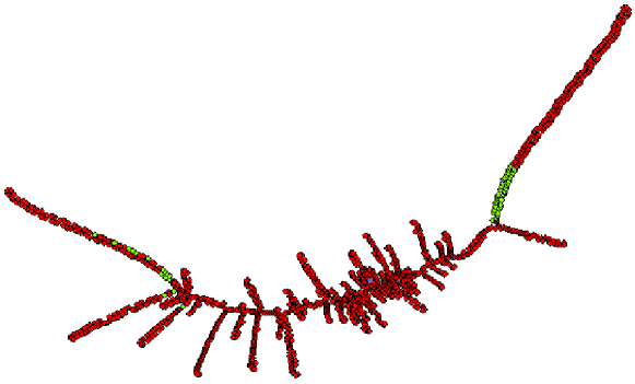
Figure 3: Community structure of the jazz musicians network. The root of the tree, in the middle of the figure, is indicated with the colour blue. The musicians with $k>170$ are indicated with green.

As in the e-mail network, the most central musicians are expected to appear at the end of the branches. However in Figure 3 we see that those musician with $k>170$ appear at the beginning of the branches. This appears to be an artefact of the manner in which the network is created, as these musicians must have played in more than one band. Therefore, their affiliation with the rest of the musicians in the branch they appear in is relatively lower. Also, since everyone plays with everyone in a band, there is no well defined central Figure.

A similar effect can be seen when analysing the bands network. The binary tree shown in Figure 4 reveals a very simple community structure. The tree is roughly divided into two large communities as expected. However, the largest branch also splits into two. To understand the origin of this division we have analysed the cities where the bands recorded. We indicate with colour red the bands that have recorded in New York. The bands that recorded in Chicago are indicated with blue.

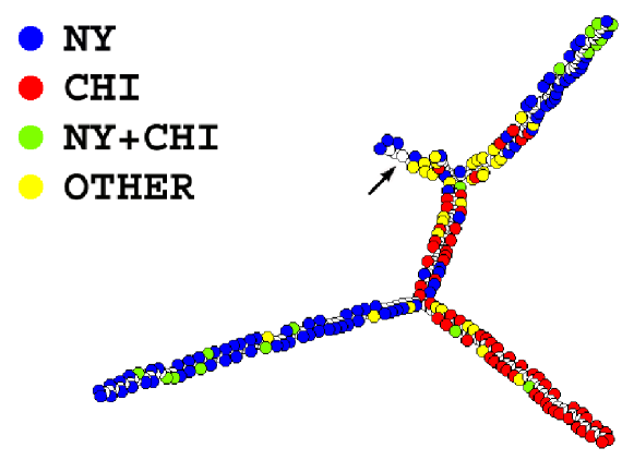
Figure 4: Communities in the jazz bands network. The arrow indicates the root of the tree. The different colours correspond to cities where a band has recorded: New York (blue), Chicago (red), both in New York and Chicago (green) and other cities (yellow).

In this case, central bands do play an important role. The analysis of names grove shows that the bands at the tip of the branches were the some of the most influential in the epoch. In general they also contained the most connected musicians.

These results show that both the musicians and bands network capture essential ingredients of the collaboration network of jazz musicians.

3.3 FisEs

We construct a network of scientists that contributed to the Statistical Physics (Física Estadística) conferences in Spain over the last 16 years. In a similar approach to the one described below, we consider two scientists linked if they have co-authored a panel contribution to any of the conference. To be able to consider the historical structure of this network we “accumulate” the network over all the conferences, that is, once a link is created, it remains, even if the authors never collaborated again. The final network (accumulated over all the years) is comprised of 784 nodes with 655 (84%) of those belonging to the giant component.

In the figure below we show the binary tree as generated by our formalism. The colours in this case represent the universities or centres of investigation of the participants. Those nodes whose affiliation has not been identified and those that belong to institutions outside of Spain are not shown, since they are few, and do not play an important role in the structure of this network. The colours in the figure represent the centres of origin of the contributors have been identified, and the grey nodes represent all universities with just a few contributions.

Figure 5: Binary tree showing the result of applying the GN algorithm and our visualisation technique to the network of coauthors in FisEs. Each branch corresponds to a real community and the tips of the branches correspond to the people that have played a major role in the different research groups. Nodes of the same colour (from the same centre) show up mainly in the same branches, showing that collaborations are more common within centres than between them.

3.4 arXiv

Finally, we study the community structure of the network of scientific collaborations as extracted from xxx.arxiv.org preprint repository newman01a . Scientists are considered linked if they have coauthored a paper in the repository. The articles defining the links are classified into different fields. Due to the size of the entire network (52909 nodes, 44337 of which are connected in a giant cluster) we create $4$ separate networks, each corresponding to one of the following fields: Mathematical Physics(math-ph), High Energy Physics - Lattice (hep-lat), General Relativity and Quantum Cosmology (gr-qc), Quantum Physics (quant-ph). An extensive study of the geographic location and thematic affiliations of the authors has not yet been performed.

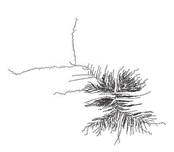
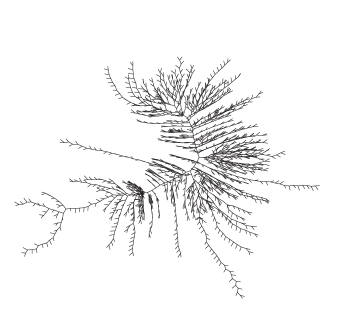
gr-qc                                                        quant-ph

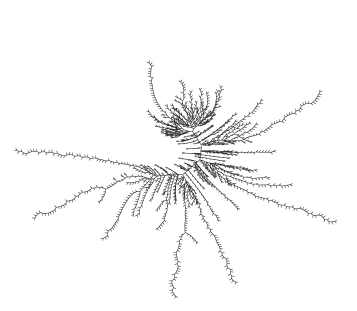
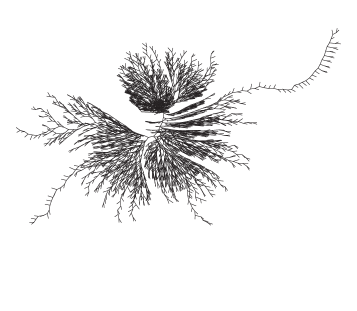
hep-lat                                                        math-ph

Figure 6: Binary trees showing the results of the community separation applied to four different parts of the arXiv network. Clear community structure is once again seen, probably corresponding to different paper themes and interests of authors, as well as geographic location.

4 Emergent properties of the community structure

In this section we characterise the statistical properties of the community structure of the networks analysed in the previous section. We will show that there are self similar properties that emerge in the network community structure.

4.1 Community size distribution

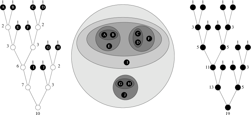
(a)                                           (b)                                           (c)

Figure 7: Community size distribution and analogy with river networks. (a) Calculation of community sizes from the binary tree. (b) Representation of the hierarchical structure of nested communities. (c) Calculation of the drainage area distribution for a river network.

The first quantity that will be considered is the community size distribution. Figure 7a represents a hypothetical tree generated by the community identification algorithm (for clarity, the tree is represented upside down). Black nodes represent the actual nodes of the original graph while white nodes are just graphical representations of groups that arise as a result of the splitting procedure. Indeed, nodes $A$ and $B$ belong to a community of size 2, and together with $E$ form a community of size 3. Similarly, $C$, $D$ and $F$ form another community of size 3. These two groups together form a higher lever community of size 6. Following up to higher and higher levels, the community structure can be regarded as the set of nested groups depicted in Figure 7b. A natural way of characterising the community structure is to study the community size distribution. In Figure 7a, for instance, there are three communities of size 2, three communities of size 3, one community of size 6, one community of size 7, and one community of size 10. Note that a single node belongs to different communities at different levels.

Figure 8 displays the heavily skewed cumulative distribution of community sizes, $P(s)$ for both the email network and the Jazz musicians network. A comparison of the shape of $P(s)$ shows a surprising similarity. In both cases, a slow, power law decay with exponent $0.48$ is observed for community sizes up to $s\sim 200$. This is followed by a faster decay and a cutoff at $s\sim 1000$ corresponding to the size of the systems (the e-mail network containing 1133 nodes and the jazz network 1265 nodes). For small values of $s$ the jazz network deviates from this behaviour, reflecting the fact that musicians are already grouped in bands of a certain size, an effect not present in the e-mail network.

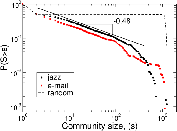
Figure 8: Cumulative community size distribution $P(S>s)$ as a function of community size $s$ for the email and jazz musician networks. The results for the e-mail network are plotted in full triangles, while full circles correspond to the jazz musicians network. The dotted line corresponds to the results obtained in a random network with the same degree distribution as the musicians network.

The power law of the above distribution suggests that there is no characteristic community size in the network (up to size 200). To rule out the possibility that this behaviour is due to our procedure we also considered the community size distribution for a random graph with the same size and degree distribution as the e-mail network. In this case (dotted line in Figure 8), $P(s)$ shows a completely different behaviour, with no communities of sizes between 10 and 600, as indicated by the plateau in Figure 8. This corresponds to a situation in which all the branches (communities) are quite small (of size less than 10) with the backbone of the network formed by the union of all these small branches.

Surprisingly, other networks studied show a power law distribution of community sizes with a different exponent. In Figure 9 we see that the exponent is very close to $-1$.

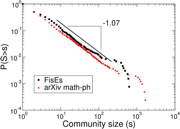
Figure 9: Cumulative community size distribution $P(S>s)$ as a function of community size $s$ for the FisEs and arXiv math-ph networks. The results for the Fises network are plotted in full squares, while full triangles correspond to the arXiv mathematical physics network. The full line is shown as a guide to the eye and follows a power law with exponent $-1.07$. Both distributions fit well to this line, up until $\sim 1000$ nodes where there is a sharp cutoff corresponding to the size of the system (784 nodes for FisEs and 2117 for math-ph).

More surprising still is the distribution of community sizes in other arXiv networks. In Figure 10 we can see a clear crosover from one scaling relation to another. All three distributions roughly follow a power law with exponent $\sim-1$ for community sizes up to $60$ nodes, whereas between $60$ and $\sim 1000$ nodes the exponent is seen to be $\sim-0.5$.

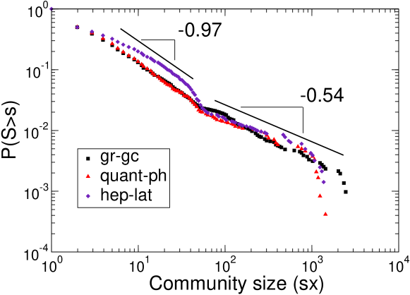
Figure 10: Cumulative community size distribution $P(S>s)$ as a function of community size $s$ for the arXiv gr-qc, quant-ph and hep-lat networks. The results for the gr-qc network are plotted in full squares, full triangles correspond to the quant-ph network and diamonds represent the hep-lat network. The full lines are shown as a guide to the eye and follow power laws with exponent $-0.97$ and $-0.54$. Also, all three distributions show a sharp cutoff corresponding to the size of the system (2546 nodes for gr-qc, 1460 for quant-ph and 1411 for hep-lat).

4.2 Analogy with river networks

Figure 8 presents a striking similarity with the distribution of community sizes and the distribution of drainage areas in river networks rinaldo93 ; rodriguez96 ; maritan96 ; banavar99 . This similarity can be understood by considering how this distribution is obtained from the community identification binary tree. Let us assign, as shown in Figure 7a, a value of 1 to all the leaves in the binary tree or, in other words, to all the nodes that represent single nodes in the original network (black nodes of the binary tree). Then, the size of a community $i$, $s_{i}$, is simply the sum of the values $s_{j_{1}}$ and $s_{j_{2}}$ of the two communities (or individual nodes), $j_{1}$ and $j_{2}$, that are the offspring of $i$. Figure 7c shows how the drainage area of a given point in a river network is calculated. Consider that at any node of the river network there is a source of 1 unit of water (per unit time). Then, the amount of water that a given node drains is calculated exactly as the community size for the community binary tree, but adding the unit corresponding to the water generated at that point: $s_{i}=s_{j_{1}}+s_{j_{2}}+1$. This quantity represents the amount of water that is generated upstream of a certain node. In this scenario, the community size distribution would be equivalent to the drainage area distribution of a river where water is generated only at the leaves of the branched structure.

The similarity between the community size distribution of the e-mail and jazz networks and the area distribution of a river network is striking (see, for instance, the data reported in maritan96 for the river Fella, in Italy). The exponent of the power law region is very similar: according to rinaldo93 , $\alpha_{river}=-0.43\pm 0.03$, while for the community size distribution we obtain $\alpha=-0.48$. Moreover, the behaviour with first a sharp decay and then a final cutoff is also shared. River networks are known to evolve to a state where the total energy expenditure is minimised kramer92 ; rinaldo93 ; sinclair96 . The possibility that communities within networks might also spontaneously organise themselves into a form in which some quantity is optimised is very appealing and deserves further investigation.

4.3 Horton-Strahler index

The similarity between the community size distribution and the drainage area distribution of river networks prompts one question: is this similarity arising just by chance or are there other emergent properties shared by community trees and river networks? To answer this question we consider a standard measure for categorising binary trees: the Horton-Strahler (HS) index, originally introduced for the study of river networks by Horton horton45 , and later refined by Strahler strahler52 . Consider the binary tree depicted in the left side of Figure 11.

(a)                                                    (b)

Figure 11: Calculation of the Horton-Strahler index. (a) Asymmetric binary tree (b) Corresponding Horton-Strahler indices of the leaves and branches. In this case there are $N_{1}=10$ branches with index 1, $N_{2}=3$ with index 2 and $N_{3}=1$ with index 3.

The leaves of the tree are assigned a Strahler index $i=1$. For any other branch that ramifies into two branches with Strahler indices $i_{1}$ and $i_{2}$, the index is calculated as follows:

$$i=\left\{\begin{array}[]{l@{\quad\quad}l}i_{1}+1&\mbox{if}\quad i_{1}=i_{2},\\ \max(i_{1},i_{2})&\mbox{if}\quad i_{1}\neq i_{2}.\end{array}\right.$$

Therefore the index of a branch changes when it meets a branch with higher index, or when it meets a branch with the same value and both of them join forming a branch with higher index (see 11b).

The number of branches $N_{i}$ with index $i$ can be determined once the HS index of each branch is known . The bifurcation ratios $B_{i}$ are then defined by $B_{i}=N_{i}/N_{i+1}$ (by definition $B_{i}\geq{2}$). When $B_{i}\approx B$ for all $i$, the structure is said to be topologically self-similar, because the overall tree can be viewed as being comprised of $B$ sub-trees, which in turn are comprised of $B$ smaller sub-trees with similar structures and so forth for all scales. River networks are found to be topologically self similar with $3<B<5$ halsey97 .

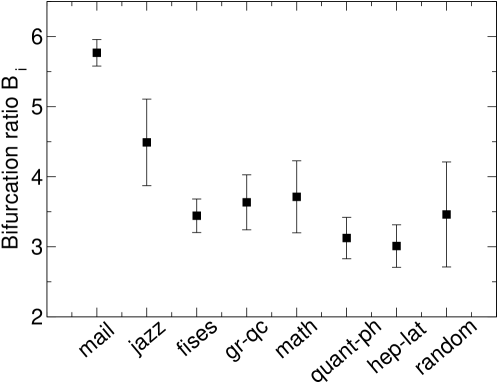
Figure 12: The Horton-Strahler bifurcation ratios $B_{i}$ and their respective errors.

We find that the community trees seen in Section 3 are topologically self similar with $3<B_{i}<5.76$ (see Figure 12). The same analysis for the communities in a random graph shows that topological self similarity does not hold, since the values of $B_{i}$ are not constant; they fluctuate more wildly around $3.46$.

The HS index also turns out to be an excellent measure to assess the levels of complexity in networks. First, let us consider the interpretation of the index in terms of communities within an organisation as represented by the email network. The index of a branch remains constant until another segment of the same magnitude is found. In other words, the index of a community changes when it joins a community of the same index. Consider, for instance, the lowest levels: individuals ($i=1$) join to form a group (with $i=2$), which in turn will join other groups to form a second level group ($i=3$). Therefore, the index reflects the level of aggregation of communities. For example, in URV one could expect to find the following levels: individuals ($i=1$), research teams ($i=2$), departments ($i=3$), faculties and colleges ($i=4$), and the whole university ($i=5$). Strikingly, the maximum HS index of the community tree is indeed 5, as shown in Figure 12.

Figure 2b shows the community tree of the e-mail network with different colours for different HS indices. This helps to distinguish the individual, team and department levels within a branch. Actually, the university level is the “backbone” of the network along which the separation of communities occurs (from the top to the bottom of the figure). From this backbone, colleges, departments and some research teams separate, although it is worth noting that colleges or, in general, centres which are small and have no internal structure will be classified with a HS index corresponding to a department or even a team. Therefore, the HS index does not represent administrative hierarchy but organisational complexity. For comparison Figure 2c shows in colour the HS index for the binary tree of a random graph.

The fact that the community structure is topologically self-similar means that the organisation is similar at different levels. In other words, it means that individuals form teams in a way that resembles very much the way in which teams join to form departments, to the way in which departments organise to form colleges, and to the way in which the different colleges join to form the whole university.

5 Conclusions

The study presented here reveals a characteristic scaling of the community size distribution of different social networks. The scaling found follows a power law with two different exponents observed for different networks. The presence of this particular type of scaling suggests that some optimising mechanism is responsible for the self-organisation of social networks. What this mechanism is, remains to be seen.

References

- (1) A. A. de Menezes and A. L. Barabasi, (2003), arXiv:cond-mat/0306304.
- (2) L. P. D. Garlaschelli, G. Caldarelli, Nature 423, 165 (2003).
- (3) M. E. J. Newman, SIAM Review 45, 167 (2003).
- (4) A. K. Jain and R. C. Dubes, Algorithms for clustering data (Prentice Hall, Englewood Cliffs, NJ, USA, 1988).
- (5) M. Girvan and M. E. J. Newman, Proc. Nat. Ac. Sci. USA 99, 7821 (2002).
- (6) S. Wasserman and K. Faust, Social Network Analysis (Cambridge University Press, Cambridge, U.K., 1994).
- (7) M. E. J. Newman, Phys. Rev. E 64, 016132 (2001).
- (8) R. Guimera et al., Phys. Rev. E, in press (2003), preprint arXiv:cond-mat/0211498.
- (9) P. Gleiser and L. Danon, Advances in Complex Systems, in press (2003), preprint arXiv:cond-mat/0307434.
- (10) L. J. Hanifan, The New Grove Dictionary of Jazz (St. Martin’s Press, New York, Boston, MA, USA, 1994).
- (11) M. E. J. Newman, Phys. Rev. E 64, 016131 (2001).
- (12) A. Rinaldo et al., Phys. Rev. Lett. 70, 822 (1993).
- (13) I. Rodriguez-Iturbe and A. Rinaldo, Fractal river basins: chance and self-organization (Cambridge University Press, Cambridge, 1996).
- (14) A. Maritan et al., Phys. Rev. E 53, 1510 (1996).
- (15) J. Banavar, A. Maritan, and A. Rinaldo, Nature 399, 130 (1999).
- (16) S. Kramer and M. Marder, Phys. Rev. Lett. 68, 205 (1992).
- (17) K. Sinclair and R. C. Ball, Phys. Rev. Lett. 76, 3360 (1996).
- (18) R. E. Horton, Bulletin of the Geological Society of America 56, 275 (1945).
- (19) A. N. Strahler, Bulletin of the Geological Society of America 63, 923 (1952).
- (20) T. C. Halsey, Europhysics Letters 39, 43 (1997).