Glassy Dynamics and Aging in Disordered
Systems
Heinz Horner
Institut für Theoretische Physik, Ruprecht-Karls-Universität Heidelberg
Philosophenweg 19, D-69120 Heidelberg, Germany
horner@tphys.uni-heidelberg.de
WE-HERAEUS-FERIENKURS FÜR PHYSIK

Collective Dynamics in Nonlinear and Disordered Systems

Chemnitz, Aug. 26. - Sept. 6. 2002

Glassy Dynamics and Aging in Disordered
Systems
Heinz Horner
Institut für Theoretische Physik, Ruprecht-Karls-Universität Heidelberg
Philosophenweg 19, D-69120 Heidelberg, Germany
horner@tphys.uni-heidelberg.de

1 Introduction

A great number of disordered systems exhibit very long relaxation times as some critical temperature is approached. Below this temperature equilibrium is no longer reached within finite time and the behaviour of such systems becomes non ergodic. Among those are diluted alloys of magnetic ions in a non magnetic matrix, so called spin-glasses [1], supercooled liquids [2] entering some glassy state at low temperature or particles moving in a random potential exhibiting a transition from diffusion to creep or pinning [3, 4]. The temporal behaviour of such systems is often referred to as glassy dynamics. Below the characteristic temperature aging is observed [5]. If, for instance, a spin-glass is cooled in a magnetic field and kept for some waiting time, the complete decay of the magnetisation after the field has been switched off, is hindered for times of the order of the waiting time. Similar phenomena are observed for the deformation of glasses under the influence of applied forces.

Glassy dynamics can also be of relevance for systems and phenomena outside physics. For some combinatorial optimisation problems simulated annealing is used in order to find good solutions. This means that some stochastic dynamics, characterized by some “temperature”, is used in order to find minima of a properly defined cost function. If such a system exhibits a freezing transition, it is not effective to spend much time in simulated annealing below this temperature and investigating the dynamics slightly above the freezing transition is much more efficient [6]. Other examples of systems of interest outside physics are models of neural networks or certain aspects of markets and other economical systems [7].

The systems mentioned above are classical. There is also interest in quantum mechanical disordered systems, for instance in certain spin-glasses or in interacting tunnelling systems being of relevance for glasses at very low temperatures. This lecture deals, however, with classical dynamical systems only.

A breakthrough of our understanding of the low temperature properties of glassy systems came from replica theory and the replica symmetry breaking scheme proposed by Parisi [8]. This theory focuses on the evaluation of the free energy averaged over some frozen disorder. The picture emerging from this theory is a decomposition of phase space into so called pure states or ergodic components, separated by barriers of infinite hight in the thermodynamic limit. Investigating the overlap among those states, an ultrametric organization reveals.

An alternative treatment of systems with quenched disorder is via dynamics [9, 10, 11, 12]. This will be the subject of this lecture. As it turns out there are many features and results common to both treatments, but there are also differences which will be discussed.

In the first part I present some of the systems of interest, in particular spin-glasses, supercooled liquids and glasses, drift, creep and pinning of a particle in a random potential, neural networks, graph partitioning as an example of combinatorial optimisation, the K-sat problem, a prototype problem from computer science, and finally the minority game as a model for the behaviour of agents on markets.

The second part deals with the dynamics of the spherical $p$-spin-glass with long ranged interactions. This model is a prototype for glassy dynamics. The equations of motion for correlation- and response-functions are derived and equilibrium solutions above the freezing temperature are investigated. Below the freezing temperature the system behaves for short time as if it were in equilibrium, for longer time its off equilibrium nature becomes apparent and correlation- and response-functions depend on waiting time. This is the manifestation of aging.

At the end of this part I discuss the so called crossover region and aging in glasses. Within mode coupling theory, which is discussed in the contribution of R. Schilling [13] in this volume, and which shows great similarity to the $p$-spin model, a dynamical transition is found at some critical temperature $T_{c}$. This is sometimes referred to as “ideal glass transition”. Comparison with experiments shows that this transition is actually smeared out and the fitted $T_{c}$ is well above the actual glass transition region. Some smearing out also results from an extended version of the mode coupling theory, which applies, however, to equilibrium only. I am going to discus a modified version of the $p$-spin model, which is able to take account for this rounding as well as aging.

2 Examples of Disordered Systems

2.1 Spin-glasses

Typical spin-glasses are diluted alloys of magnetic ions in a non magnetic matrix, e.g. $Ag_{1-x}Mn_{x}$ with $x\sim 3\%$. The magnetic ions interact via the RKKY-interaction which is mediated through the conduction electrons. It is of the form

$$J(r)\sim r^{-3}\cos(k_{f}r)$$ (1)

shown in Fig.1. For random distances $r_{ij}$ between pairs of magnetic ions, their exchange interactions $J_{ij}\!=\!J(r_{ij})$ are also random variables including positive and negative values. This leads to frustration, as shown in the insert of Fig.1 for a triple $i\,j\,k$ of ions with $J_{ij}>0$, $J_{i,k}>0$ and $J_{j,k}<0$.

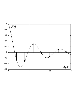
Figure 1: RKKY-interaction

At high temperatures spin-glasses typically show a Curie-law for the magnetic susceptibility $\chi\sim 1/T$, as shown in Fig.2 for $\underline{\rm Cu}{\rm Mn_{x}}$. Below some freezing temperature $T_{g}$ the system is no longer in equilibrium. If the system is cooled in a small field, the magnetisation $M=\chi_{FC}B$ stays more or less constant ($a$ and $c$ in Fig.2). The ratio $\chi_{FC}=M/B$ is called field cooled susceptibility.

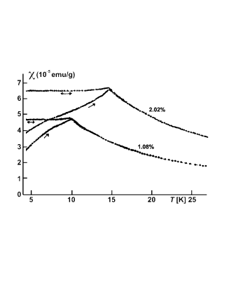
Figure 2: Susceptibility of $\underline{\rm Cu}{\rm Mn_{x}}$ [14] for different values of the concentration $x$ of the magnetic ions.

If, however, the system is cooled without applied field, and the field is applied only after some waiting time $t_{w}$, the resulting magnetisation is reduced, i.e. the zero field cooled susceptibility $\chi_{ZFC}=M/B<\chi_{FC}$ ($b$ and $d$ in Fig.2). Approaching the critical temperature $T_{g}$ critical slowing down can be observed, see Fig.3.

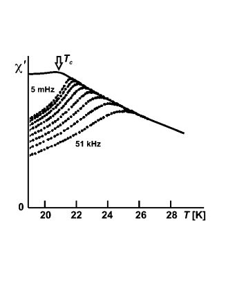
Figure 3: Real part of the susceptibility $\chi^{\prime}(\omega)$ for ${\rm Fe_{0.5}MN_{0.5}TiO_{3}}$ [15]. The critical temperature is $T_{g}=20.7\,{\rm[K]}$

The off equilibrium character of the low temperature phase is most clearly demonstrated by the decay of the remnant magnetisation. In this experiment the sample is rapidly cooled in a magnetic field to a temperature $T<T_{g}$. After some waiting time $t_{w}$ the field is switched off, and the decay of the magnetisation is observed as function of time $t$ elapsed after removal of the field. Following some rapid initial decay, not shown in Fig.4, the magnetisation stays almost constant up to time $t\sim t_{w}$.

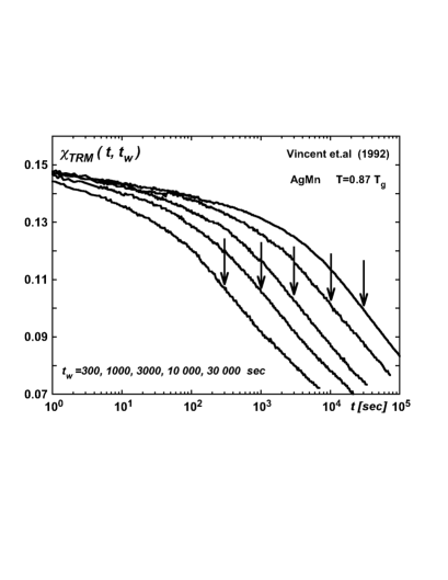
Figure 4: Decay of the remnant magnetisation for various waiting times $t_{w}$ indicated by arrows [16].

Investigating more elaborate temperature programs $T(t)$ a variety of other striking memory and aging effects are observed [17]. Similar aging phenomena are also found in glasses [5].

Theoretical investigations are typically based on Ising models with random interactions. Their energy is

$$H=-\mbox{$\frac{1}{2}$}\sum_{i,j}J_{i,j}\sigma_{i}\sigma_{j}\qquad\quad\sigma_{i}=\pm 1.$$ (2)

The interactions $J_{ij}$ are assumed to be gaussian distributed random variables with

$$\overline{J_{i,j}}=0\qquad\quad\overline{J_{i,j}J_{k,l}}=\mbox{$\frac{1}{2}$}\{\delta_{i,k}\delta_{j,l}+\delta_{i,l}\delta_{j,k}\}W_{i,j}.$$ (3)

Calculating e.g. the free energy

$$F=-k_{B}T\,\overline{\ln\Big{(}\sum_{\{\sigma=\pm 1\}}\mbox{e}^{-\beta H}\Big{)}}^{J}$$ (4)

the problem arises, that the logarithm of the partition function has to be averaged over the gaussian disorder. Similar problems exist in evaluating expectation values, e.g.

$$\left\langle{\sigma_{i}\sigma_{j}}\right\rangle=\overline{\Big{(}\sum_{\{\sigma\}}\sigma_{i}\sigma_{j}\mbox{e}^{-\beta H}\Big{)}\Big{/}\Big{(}\sum_{\{\sigma\}}\mbox{e}^{-\beta H}\Big{)}}^{J}.$$ (5)

This can be done using the replica trick [8].

As an alternative, one can examine dynamics in the form of stochastic processes having the Boltzmann distribution $\sim\mbox{e}^{-\beta H}$ as stationary solution. For an Ising model, Glauber dynamics can be used. It is is given by a single spin-flip master-equation such that

$$\frac{\mbox{d}}{\mbox{d}t}\left\langle{\sigma_{i}(t)}\right\rangle=\left\langle{\tanh\Big{(}\beta\sum_{i}J_{i,j}\sigma_{j}(t)\Big{)}}\right\rangle.$$ (6)

Using a path integral representation of this process, the average over the stochastic interactions can easily be performed. This will be subject of the second part of this lecture.

2.2 Supercooled Liquids and Glasses

If a liquid is cooled sufficiently slow, it may avoid crystallisation and enter the state of a supercooled liquid. With decreasing temperature the shear viscosity $\eta(T)$ increases and reaches a value of $\eta(T_{g})\approx 10^{12}\,{\rm[Pa\,sec]}$ defining the glass temperature $T_{g}$. At this value, plastic flow can hardly be observed in laboratory experiments. In some glasses, so called strong glasses, the viscosity follows more or less an Arrhenius law $\eta(T)\sim\mbox{e}^{\beta E_{a}}$ [18]. A typical strong glass formers is ${\rm SiO_{2}}$ with an activation energy $E_{a}\approx 4\,{\rm eV}$ corresponding to the binding energy of a covalent bond. Fragile glass formers, on the other hand, show pronounced deviations from this law. Typical examples are organic molecular glasses, ionic glasses, polymers or proteins. Some examples are shown in Fig.5.

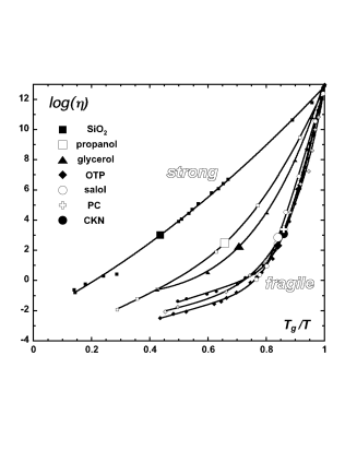
Figure 5: Angell plot: Logarithm of the viscosity versus inverse temperature [18]. A straight line corresponds to Arrhenius behaviour. The fat symbols indicate the MCT-crossover temperature $T_{c}$ [19].

There are other attempts to define a glass transition temperature, e.g. identifying a rapid drop in the specific heat or thermal expansion [20]. Actually the glass temperature defined in one way or another usually depends on the cooling rate, and it is not clear at all, if some finite $T_{g}$ exists in real glasses. There is no need to discuss this further in this lecture, since theories of the structural glass transitions are covered in the contribution of R. Schilling [13] in this volume.

There is, however, one aspect of interest in the present context. This is the ”Ideal Glass Transition” found in mode coupling theory (MCT) [19, 13]. The resulting equations resemble those found for the dynamics of spherical $p$-spin interaction spin-glass [21, 22] to be discussed later in this lecture. This theory yields diverging time scales as some critical temperature $T_{c}$ is approached, and non ergodic behaviour for $T<T_{c}$.

An onset of critical slowing down, usually referred to as $\alpha$-relaxation, can be observed in fragile glasses, e.g. in the dielectric susceptibility $\chi^{\prime\prime}(\omega)$ of the ionic glass CKN [23] shown in Fig.6.a. Fitting the critical temperature $T_{c}$ and other parameters of mode coupling theory, as indicated in Fig.6.b, yields the critical temperatures shown in Fig.5.

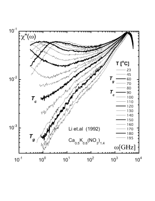
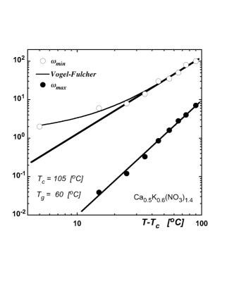
(a)                                                (b)

Figure 6: (a) Imaginary part of the dielectric susceptibility $\chi^{\prime\prime}(\omega)$ of the ionic glass CKN [23]. The $\alpha$-relaxation shows up as the broad peak at the lower frequency. (b) The frequencies of the maximum $\omega_{\rm max}$ and minimum $\omega_{\rm min}$ of $\chi^{\prime\prime}(\omega)$ fitted to   $\omega_{\rm max}\sim(T-T_{c})^{\eta}$  and  $\omega_{\rm min}\sim(T-T_{c})^{\eta^{\prime}}$.

Actually an extended version of the mode coupling theory [19, 24] yields a rounding of the singularity near $T_{c}$ and equilibrium behaviour for temperatures below $T_{c}$, in contrast to the findings of the simplified mode coupling theory or the $p$-spin-glass. On the other hand, aging can be observed in glasses as well, indicating off equilibrium properties at low temperatures. An example is shown in Fig.7. We shall come back to this point later.

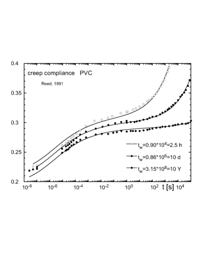
Figure 7: Aging observed in PVC [25]. A shear stress is applied after some waiting time $t_{w}$ following a quench from the liquid state. Then the resulting deformation is observed as function of time $t$.

Assuming pair interactions, the (potential) energy may be written as

$$H=\mbox{$\frac{1}{2}$}\!\int\!\mbox{d}\vec{r}\mbox{d}\vec{r^{\prime}}\,V(\vec{r}-\vec{r^{\prime}})\,n(\vec{r})\,n(\vec{r^{\prime}})$$ (7)

where $n(\vec{r})$ is the density at point $\vec{r}$.

If one is interested in slow dynamics only, it is sufficient to investigate the limit of overdamped motion, i.e. the Langevin equation

$$\frac{\partial}{\partial t}n(\vec{r},t)=\vec{\nabla}n(\vec{r},t)\cdot\vec{\nabla}\!\int\!\mbox{d}\vec{r^{\prime}}\,V(\vec{r}-\vec{r^{\prime}})\,n(\vec{r^{\prime}},t)+\vec{\eta}(\vec{r},t)\cdot\vec{\nabla}n(\vec{r},t)$$ (8)

with fluctuating forces such that

$$\left\langle{\vec{\eta}(\vec{r},t)}\right\rangle=0\qquad\quad\left\langle{\vec{\eta}(\vec{r},t)\cdot\vec{\eta}(\vec{r}^{\prime},t^{\prime})}\right\rangle=2\,T\,\delta(\vec{r-r}^{\prime})\,\delta(t-t^{\prime}).$$ (9)

Investigating time dependent correlation-functions, the nonlinear term in the above equation is treated via mode coupling theory. As mentioned, the resulting equations of motions are identical to those obtained for the $p$-spin-glass (in equilibrium). This is remarkable, because the Hamiltonian of the spin-glass has built in quenched disorder, whereas the Hamiltonian of the glass does not, and the disorder appears to be self generated.

The relevance of the findings of mode coupling for a glass transition at $T_{g}$ is not completely obvious. Other concepts have been proposed to understand the glass transition, e.g. activated transitions among “inherent states” [26] or models with kinetically constraint dynamics [27, 28].

2.3 Motion of a particle (manifold) in a random potential

Another example for glassy dynamics is the motion of a particle in a correlated random potential [3, 4]. Using again the limit of strong damping, a Langevin equation may be used

$$\vec{v}(t)=\frac{\mbox{d}}{\mbox{d}t}\vec{r}(t)=-\vec{\nabla}V(\vec{r}(t))+\vec{K}+\vec{\eta}(t)$$ (10)

where $V(\vec{r})$ is assumed to be a gaussian random potential with moments

$$\overline{V(\vec{r})}=0\qquad\overline{V(\vec{r})\,V(\vec{r}^{\prime})}=\frac{V_{o}}{(|\vec{r}-\vec{r}^{\prime}|+a)^{\gamma}}\,,$$ (11)

and $\vec{K}$ is some external force pulling the particle. The thermal noise is again given by Eq.(9).

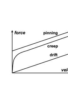
Figure 8: Drift, creep and pinning for a particle moving in a random potential.

Depending on temperature $T$ and the exponent $\gamma$, characterising the range of the random potential, various types of motion are found [4], see Fig.8. For $T>T_{c}(\gamma)$ the average velocity $v(K)\sim K$, i.e. there is a finite friction constant. For $T<T_{c}(\gamma)$ and $\gamma<\gamma_{c}$ the particle moves only if the force exceeds some critical value $K>K_{\rm pinning}(T,\gamma)$. For $T<T_{c}(\gamma)$ and $\gamma>\gamma_{c}$ creep is found, i.e. $v(K)\sim K^{\eta}$ with $\eta<1$.

A similar freezing transition shows up for a chain or some other manifold moving in a random potential [29].

2.4 Neural Networks

Considerable effort has been put into the study of formal neural networks dealing with random patterns [30], e.g. the Hopfield model [31] as a prototype of an associative memory.

Representing the “on” and “off” state of a neuron by the two states of an Ising spin $\sigma_{i}=\pm 1$, the energy is assumed to be that of an Ising spin-glass Eq.(2). The couplings $J_{i,j}$ are, however, determined by the patterns to be memorised. Let $\xi_{i}^{\mu}=\pm 1$ be a set of random patterns, where $i=1\cdots N$ labels the neurons and $\mu=1\cdots A$ the patterns. Then the choice of the couplings $J_{i,j}$ such that

$$J_{i,j}=\mbox{$\frac{1}{N}$}\sum_{\mu}\xi_{i}^{\mu}\xi_{j}^{\mu}$$ (12)

ensures, that a fixed point of the dynamics, defined by Eq.(6), exists near each pattern $\mu$ at least as long as $A<\alpha_{c}N$ with $\alpha_{c}\approx 0.13$. Each fixed point is surrounded by some basin of attraction, i.e. if the initial state contains a sufficient part of a pattern, the complete pattern is reconstructed with a small number of errors. The size of the basin of attraction depends on the loading $\alpha=A/N$ [32]. For $\alpha>\alpha_{c}$ the memory is overloaded and looses its function completely. The dynamics becomes glassy, which is not too surprising, since the couplings $J_{i,j}$ can be positive as well as negative, resulting in frustration.

Methods developed for spin-glasses, replica theory and dynamics, have also been used to investigate this and other types of neural networks. In particular bounds of learning [30, 6] have been determined.

2.5 Combinatorial Optimisation Problems

Combinatorial optimisation problems show up in various technical applications. The problem is, to find the “best” out of a discrete set of states. Finding the ground state of an Ising spin-glass or solving the travelling sales man problem, i.e. finding the shortest path connecting a set of towns, are examples. In many cases the problem is $NP$-complete, i.e. the optimal solution can not be found with computational effort growing with the size $N$ of the problem to some power. This means that for larger systems it is virtually impossible to find the optimal solution. In many applications it might, however, be sufficient to find good solutions in polynomial time. One of the standard procedures is simulated annealing [33]. It is implemented by constructing a cost function (energy), and using some stochastic dynamics, characterised by a temperature. This temperature is slowly decreased, and hopefully states with low values of the cost function are found.

Actually such a system might undergo a transition to glassy dynamics below some critical temperature $T_{c}$. If this is the case, extending simulated annealing to $T<T_{c}$ is not efficient, and searching for good solutions at $T\approx T_{c}$ is more effective [6].

A standard problem in this context is graph bipartitioning [34]. Assume electronic components $i=1\cdots N$ have to be placed on two chips $A$ and $B$. The aim is to place them such that the number of connections between $A$ and $B$ is minimal. A cost function for this problem can be defined by mapping it to an Ising system with

$$\sigma_{i}=1\quad{\rm if\;\;}i{\rm\;\;on\;\;}A\qquad\sigma_{i}=-1\quad{\rm if\;\;}i{\rm\;\;on\;\;}B.$$ (13)

and interactions

$$J_{ij}=1\quad{\rm if\;\;}i{\rm\;\;and\;\;}j{\rm\;\;are\,connected}\qquad J_{i,j}=0\quad{\rm else}.$$ (14)

The resulting cost function is

$$H=-\mbox{$\frac{1}{2}$}\sum_{i,j}J_{i,j}\,\sigma_{i}\,\sigma_{j}.$$ (15)

For the process of simulated annealing again Glauber dynamics, Eq.(6), may be used.

2.6 Random $K$-sat Problem

Another standard $NP$-problem is the $K$-sat problem [35]. This problem deals with $N$ Boolean variables represented by $\sigma_{i}=\pm 1$. There are $A$ clauses with $K$ literals per clause among the Boolean variables or their negations, e.g. for $K=3$:  $R=\{\,\sigma_{i}$ OR $\sigma_{j}$ OR NOT $\sigma_{k}\,\}$. A clause $R_{\mu}(\{\sigma\})$ can be represented as

$$\xi_{i}^{\mu}=\left\{\begin{array}[]{rrcl}1&\;\;{\rm if}&\;\sigma_{i}&\;{\rm in}\;\;R_{\mu}\\ -1&\;\;{\rm if}&\;\;{\rm NOT}\,\sigma_{i}&\;{\rm in}\;\;R_{\mu}\\ 0&&\;\;{\rm else}\,.\\ \end{array}\right.$$ (16)

The clause $R_{\mu}(\{\sigma\})$ is not fulfilled if  $\displaystyle\sum_{i=1}^{N}\xi_{i}^{\mu}\sigma_{i}=K$, and a cost function

$$H=\sum_{\mu=1}^{A}\delta\Big{(}\sum_{i=1}^{N}\xi_{i}^{\mu}\sigma_{i}-K\Big{)}\qquad{\rm or}\qquad H=\sum_{\mu}\Big{(}\sum_{i=1}^{N}\xi_{i}^{\mu}\sigma_{i}-K\Big{)}^{2}$$ (17)

may be used. Finding solutions of the $K$-sat problem, again simulated annealing can be used, and finding a ground state with $H=0$ means that the corresponding choice of the Boolean variables satisfies all clauses. The formal similarity to the Hopfield model is obvious. For random clauses $\xi_{i}^{\mu}$ a critical $\alpha_{c}(K)$ exists, such that for $\alpha=A/K<\alpha_{c}(K)$ solutions can typically be found by the polynomial simulated annealing procedure.

2.7 Minority game

Methods, developed for disordered systems, have also been applied to various problems in economy, especially concerning financial markets. Activities of this kind are usually subsummized under the notion econophysics. As an example the minority game [7] is discussed. This is a repeated game, where $N$ agents have to decide which of two actions, e.g. buy or sell, to take. The goal is to be in the minority. Each agent knows the outcome of the last $L$ games and can select among two strategies, where the set of strategies is different for each agent. For each new game the agent selects the strategy which would have been most successful over the last $L$ games. Again this problem can be mapped onto the dynamics of an Ising spin system with quenched disorder, the disorder being the random set of strategies for each agent. Depending on $N$ and $L$ freezing transitions are found.

3 Dynamics of the $p$-Spin Interaction Spin-Glass

3.1 Soft Spin Models

In the previous part of this lecture we have seen many different examples of disordered systems exhibiting transitions to glassy dynamics and off equilibrium behaviour. Some of these systems are based on Glauber dynamics with transition probabilities among a discrete set of states. Glauber dynamics is very appropriate for Monte-Carlo simulations, but difficult for analytic investigations [6]. In the following we therefore investigate a model based on continuous degrees of freedom. In equilibrium the resulting equations of motion are identical to those derived from mode coupling theory for glasses [13, 19]. The model is, however, more general in the sense that it allows to study off equilibrium properties and aging [5].

Actually we investigate a whole class of models. The degrees of freedom are $N$ scalar real variables $\varphi_{i}$ representing soft spins or other variables. The energy (Hamiltonian) is

$$H=\sum_{i}U(\varphi_{i})-\sum_{i}h_{i}\varphi_{i}-\mbox{$\frac{1}{2}$}\sum_{i,j}J_{ij}\varphi_{i}\varphi_{j}-\mbox{$\frac{1}{3!}$}\sum_{i,j,k}J_{ijk}\varphi_{i}\varphi_{j}\varphi_{k}-\cdots$$ (18)

where $U(\varphi)$ is some local potential constraining the distribution of the $\varphi_{i}$. Ising spins for instance can be approximated by choosing $U(\varphi)$ as deep double well potential with minima at $\varphi=\pm 1$, e.g. $U(\varphi)=\overline{U}\,(1-\varphi^{2})^{2}$. For a spherical model $U(\varphi)=\mbox{$\frac{1}{2}$}\mu\varphi^{2}$ with $\mu$ such that $\left\langle{\varphi^{2}}\right\rangle=1$.

We allow for multi spin interactions $J_{ijk}\cdots$ involving two and more spins or particles. The interactions are Gaussian random variables with

$$\overline{J_{ij}}=0\hskip 41.25648pt\overline{J_{ij}J_{kl}} = \mbox{$\frac{1}{2}$}\{\delta_{i,k}\delta_{j,l}+\delta_{i,l}\delta_{j,k}\}\,W^{\{2\}}_{ij}$$

$$\overline{J_{ijk}}=0\hskip 28.45274pt\overline{J_{ijk}J_{lmn}} = \mbox{$\frac{1}{3!}$}\{\delta_{i,l}\delta_{j,m}\delta_{k,n}+\cdots\}\,W^{\{3\}}_{ij}$$ (19)

$$\cdots\hskip 70.56284pt\cdots$$

For real spin-glasses the range of the interactions is finite, and one may choose $W^{(2)}_{ij}=W$ if site i and j are next neighbours and $W^{(p)}_{\cdots}=0$ else (Edwards-Anderson model [36]). For the SK-model (Sherrington-Kirkpatrick [37]) on the other hand interactions with unlimited range are used. Models with long ranged interactions (or models in infinite dimensions) have the advantage that mean field theory yields the exact solution. For other problems like neural networks or combinatorial optimisation problems space has no meaning and interactions among all elements are appropriate. The strength of the interactions has to scale with the number $N$ of elements in order to allow for a non trivial thermodynamic limit $N\to\infty$

$$W^{(p)}_{\cdots}=N^{-p/2}\,W_{p}.$$ (20)

Models of this kind are often referred to as mean field models.

3.2 Replica Theory

Equilibrium properties can be derived from the free energy averaged over the disorder

$$F(T,h)=-k_{B}\,T\,\overline{\ln\,Z(T,h,J)}^{J}.$$ (21)

The problem is to perform the average of the logarithm of the partition function instead of averaging the partition function itself and taking the logarithm afterwards. The replica trick [8, 37] uses the identity

$$\ln(x)=\lim_{n\to 0}\Big{(}x^{n}-1\Big{)}.$$ (22)

For integer $n$ the partition function $Z^{n}$ may be computed by replicating the system $n$ times

$$Z^{n}=\prod_{\alpha=1}^{n}\int\mbox{d}\varphi_{1}^{\alpha}\cdots\mbox{d}\varphi_{N}^{\alpha}\,\mbox{e}^{-\beta\sum_{\alpha}H(\varphi^{\alpha})}.$$ (23)

This quantity can now be averaged easily over the gaussian disorder. Since the disorder is the same for each of the replica, the resulting effective Hamiltonian

$$-\beta{\cal H}=-\beta\sum_{\alpha}\overline{H(\varphi_{\alpha})}^{J}+\mbox{$\frac{1}{2}$}\beta^{2}\sum_{\alpha,\beta}\Big{\{}\overline{H(\varphi_{\alpha})H(\varphi_{\beta})}^{J}-\overline{H(\varphi_{\alpha})}^{J}\,\overline{H(\varphi_{\beta})}^{J}\Big{\}}$$ (24)

couples different replica. The partition function $Z^{n}$ can be evaluated for mean field models introducing the order parameters

$$q_{\alpha,\beta}=\overline{\left\langle{\varphi_{i}^{\alpha},\varphi_{i}^{\beta}}\right\rangle}^{J}.$$ (25)

The problem is symmetric with respect to permutations of the replica. At high temperatures $T>T_{c}$ the order parameters are symmetric with respect to permutations as well, i.e.

$$q_{\alpha,\beta}=q_{0}\delta_{\alpha,\beta}+q\,\Big{(}1-\delta_{\alpha,\beta}\Big{)}.$$ (26)

At low temperatures $T<T_{c}$ two different replica symmetry breaking schemes have been proposed [8], a one step symmetry breaking and alternatively a hierarchical symmetry breaking in $p$ steps with $p\to\infty$, the so called full symmetry breaking. At the end the limit $n\to 0$ has to be taken extrapolating the results obtained originally for integer $n$ to real $n$. The results for the low temperature state with full symmetry breaking are interpreted in terms of a state composed of distinct pure states with ultrametric organisation with respect to their overlap. Pure states are interpreted as regions of phase space, valleys, surrounded by barriers of infinite hight. Within each valley the system is in equilibrium. A corresponding interpretation is obtained from the following investigation of dynamics. For further details on the replica theory and results see [8, 13].

3.3 Langevin Dynamics and Path Integrals

An investigation of dynamics yields additional information about the temporal behaviour of correlations and especially about the critical slowing down at the freezing transition. Below the transition temperature $T<T_{c}$ signatures of non equilibrium are expected, in particular aging.

Specifying a Hamiltonian for a classical system does not specify its dynamics uniquely. The dynamics has, however, to be chosen such that the equilibrium state   $\sim\mbox{e}^{-\beta H}$ is stationary. The simplest form is a Langevin equation corresponding to the overdamped motion of particles or spins

$$\frac{\mbox{d}\varphi_{i}(t)}{\mbox{d}t}=-\frac{\delta H(\{\varphi(t)\})}{\delta\varphi_{i}(t)}+\eta_{i}(t)=F_{i}(\{\varphi(t)\})+\eta_{i}(t)$$ (27)

where the friction constant has been put to 1. The fluctuating forces, representing a heat bath, are assumed to be Gaussian distributed random variables with

$$\left\langle{\eta_{i}(t)}\right\rangle=0\qquad\quad\left\langle{\eta_{i}(t)\eta_{j}(t^{\prime})}\right\rangle=2\,T\,\delta_{i,j}\,\delta(t-t^{\prime}).$$ (28)

In contrast to the quenched disorder of the interactions $J_{\cdots}$, the fluctuating forces $\eta_{i}(t)$ depend on time. Averages over the $J_{\cdots}$ and the thermal motion, are distinguished by different notations, $\overline{\cdots}^{J}$ and $\left\langle{\cdots}\right\rangle$, respectively.

It is convenient, especially in view of the average over the quenched disorder, to introduce a path integral representation [38]. In the following the derivation is outlined, dropping the site index $i$ for a moment. Let

$$\varphi(t)=\varphi(t;\{\eta\};\varphi_{0})$$ (29)

be solution of Eq.(27) with initial condition $\varphi(t_{0})=\varphi_{0}$. The thermal average of a product of $\varphi$-variables at different time is then

$$\left\langle{\varphi(t)\varphi(t^{\prime})\cdots}\right\rangle=\!\int\!\mbox{d}\varphi_{0}P_{0}(\varphi_{0})\!\int\!\!\!\int_{t_{0}}\!\!{\cal D}\{\eta\}\,\mbox{e}^{{\cal W}(\{\eta\};t_{0})}\varphi(t;\{\eta\};\varphi_{0})\,\varphi(t^{\prime};\{\eta\};\varphi_{0})\cdots$$ (30)

with

$${\cal W}(\{\eta\};t_{0})=-\mbox{$\frac{1}{4T}$}\int_{t_{0}}\mbox{d}t\,\eta(t)^{2}.$$ (31)

$P_{0}(\varphi_{o})$ is some distribution of initial values.

Instead of integrating over the fluctuating forces $\eta(t)$, it would be more convenient to have a path integral over the dynamical variables $\varphi(t)$. This can be done by introducing imaginary auxiliary variables $\hat{\varphi}(t)$, and then

$$\left\langle{\varphi(t)\varphi(t^{\prime})\cdots}\right\rangle=\!\int\!\mbox{d}\varphi_{0}P_{0}(\varphi_{0})\!\int\!\!\!\int_{t_{0}}\!\!{\cal D}\{\hat{\varphi},\varphi,\eta\}\,\mbox{e}^{{\cal W}(\{\hat{\varphi},\varphi,\eta\};t_{0})}\varphi(t)\,\varphi(t^{\prime})\cdots$$ (32)

with

$${\cal W}(\{\hat{\varphi},\varphi,\eta\};t_{0})=-\int_{t_{0}}\!\mbox{d}t\,\Big{\{}\mbox{$\frac{1}{4T}$}\eta(t)^{2}+\hat{\varphi}(t)\Big{[}\dot{\varphi}(t)-F(\varphi(t))-\eta(t)\Big{]}\Big{\}}.$$ (33)

The path integral over the auxiliary imaginary variables $\hat{\varphi}(t)$ can be viewed as a product of $\delta$-functions insuring the fulfilment of the equation of motion, Eq.(27), at all time.

The final step is to integrate over the fluctuating forces $\eta(t)$, which can easily be done by completing the square in Eq.(33), and now

$$\left\langle{\varphi(t)\varphi(t^{\prime})\cdots}\right\rangle=\!\int\!\mbox{d}\varphi_{0}P_{0}(\varphi_{0})\!\int\!\!\!\int_{t_{0}}\!\!{\cal D}\{\hat{\varphi},\varphi\}\,\mbox{e}^{{\cal W}(\{\hat{\varphi},\varphi\};t_{0})}\varphi(t)\,\varphi(t^{\prime})\cdots$$ (34)

with

$${\cal W}(\{\hat{\varphi},\varphi\};t_{0})=\int_{t_{0}}\!\mbox{d}t\,\Big{\{}T\hat{\varphi}(t)^{2}-\hat{\varphi}(t)\Big{[}\dot{\varphi}(t)-F(\varphi(t))\Big{]}\Big{\}}.$$ (35)

The path integral extends over real functions $\varphi(t)$ with initial condition $\varphi(t_{0})=\varphi_{0}$, and imaginary functions $\hat{\varphi}(t)$ with unrestricted initial conditions. The path integral goes over functions in the interval $t_{0}<t<t_{1}$ with $t_{1}$ greater than the latest time argument in the expectation value Eq.(34).

The auxiliary fields have a physical interpretation. Allowing for a time dependent external field $h(t)$ in Eq.(18), response functions can be expressed as expectation values of the original and auxiliary fields, e.g.

$$\frac{\delta\left\langle{\varphi(t)}\right\rangle}{\delta h(t^{\prime})}=\left\langle{\varphi(t)\hat{\varphi}(t^{\prime})}\right\rangle.$$ (36)

The expectation value on the right hand side is of the form Eq.(34). The auxiliary fields are therefore denoted as response fields.

Response functions have to be causal, i.e. Eq.(36) has to vanish for $t^{\prime}\geq t$. This is in accordance with the Ito calculus for the stochastic equation of motion Eq.(27), assuming that the action of the forces is retarded [38, 22].

The formulation given above is completely general in the sense that it is not restricted to equilibrium or small deviations from equilibrium. In general correlation- and response-functions are not related. In equilibrium, however, they have to obey fluctuation-dissipation-theorems (FDT)

$$\beta\,\frac{\mbox{d}}{\mbox{d}t^{\prime}}\,q(t,t^{\prime})=r(t,t^{\prime})$$ (37)

where correlation- and response-function are defined as

$$q(t,t^{\prime})=\left\langle{\varphi(t)\varphi(t^{\prime})}\right\rangle\qquad\quad r(t,t^{\prime})=\left\langle{\varphi(t)\hat{\varphi}(t^{\prime})}\right\rangle.$$ (38)

A sketch of the proof is as follows: The first step is to show that for equilibrium initial condition

$$P_{0}(\varphi_{0})=Z^{-1}\mbox{e}^{-\beta H(\varphi_{0})}$$ (39)

the initial time is arbitrary as long as it is earlier than the earliest time in expectation values of the type Eq.(34) or Eq.(36). Assume that the initial distribution at some time $t_{0}^{\prime}<t_{0}$ is given by Eq.(39). For $t^{\prime}_{0}<t<t_{0}$ one replaces $\hat{\varphi}(t)\to\hat{\varphi}(t)+\beta\dot{\varphi}(t)$ in the path integral Eq.(34) and in the action Eq.(35). This results in

$${\cal W}(\{\hat{\varphi},\varphi\};t_{0})-{\cal W}(\{\hat{\varphi},\varphi\};t^{\prime}_{0}) = \int_{t^{\prime}_{0}}^{t_{0}}\!\mbox{d}t\,\Big{\{}T\hat{\varphi}(t)^{2}+\hat{\varphi}(t)\Big{[}\dot{\varphi}(t)+F(\varphi(t))\Big{]}\Big{\}}\quad$$ (40)

$$- \beta H(\varphi(t_{0}))+\beta H(\varphi(t^{\prime}_{0})).$$

The last two terms in Eq.(40) originate from integrating a contribution $\beta\dot{\varphi}(t)F(\varphi(t))=-\beta\mbox{d}H(\varphi(t))/\mbox{d}t$ which appears if the above substitution is performed. Evaluating the path integral over $\varphi(t)$ or actually $\dot{\varphi}(t)$ for $t^{\prime}_{0}<t<t_{0}$ the only contributions come from $\hat{\varphi}(t)=0$. The last two terms in Eq.(40) replace the initial equilibrium condition Eq.(39) at $t^{\prime}_{0}$ by the corresponding one at $t_{0}$. If the system is ergodic, the limit $t^{\prime}_{0}\to-\infty$ may be taken and, as a consequence, the initial condition becomes irrelevant.

Consider now a small change of the external field $\delta h(t)=\delta h_{0}$ for $t<t_{0}$ and $\delta h(t)=0$ for $t>t_{0}$. Assuming equilibrium

$$\frac{\delta\left\langle{\varphi(t)}\right\rangle}{\delta h_{0}}=\int_{-\infty}^{t_{0}}\!\!\mbox{d}t^{\prime}\,r(t,t^{\prime})=\beta q(t,t_{0}).$$ (41)

For the first expression the initial time $t^{\prime}_{0}\to-\infty$ is used. The second is obtained by differentiating the equilibrium initial condition at $t_{0}$ with respect to $h$. The FDT is obtained by differentiation both expressions of Eq.(41) with respect to $t_{0}$.

Deriving this result no explicit time dependence of the Hamiltonian is allowed and the system has to be ergodic.

3.4 Average over Quenched Disorder

As pointed out already in the context of the replica theory, the calculation simplifies considerably for mean field models with long ranged interactions, specified in Eq.(20). In the following we investigate models of this kind [9, 10, 21, 22].

Provided the initial condition does not depend on the disorder, the average over the interactions $J^{(p)}_{\cdots}$ can easily be performed using the general relation

$$\overline{\mbox{e}^{ax}}=\mbox{e}^{a\overline{x}+\frac{1}{2}\overline{(x-\overline{x})^{2}}}$$ (42)

valid for Gaussian distributions. This yields, for the Hamiltonian Eq.(18) and the disorder specified in Eq.(3.1) and Eq.(20), the effective action

$$\overline{{\cal W}(\{\hat{\varphi},\varphi\})}^{J} = \int\!\!\mbox{d}t\sum_{i}\Big{\{}T\hat{\varphi}_{i}(t)^{2}-\hat{\varphi}_{i}(t)\Big{[}\dot{\varphi}_{i}(t)-h-U^{\prime}\big{(}\varphi_{i}(t)\big{)}\Big{]}\Big{\}}$$

$$+ \int\!\!\mbox{d}t\!\!\int^{t}\!\!\mbox{d}t^{\prime}\sum_{i}\Big{\{}\hat{\varphi}_{i}(t)W^{\prime}\Big{(}\mbox{$\frac{1}{N}$}\sum_{j}\varphi_{j}(t)\varphi_{j}(t^{\prime})\Big{)}\hat{\varphi}_{i}(t^{\prime})$$

$$\hskip 4.2679pt+\hat{\varphi}_{i}(t)\mbox{$\frac{1}{N}$}\sum_{j}\varphi_{j}(t)W^{\prime\prime}\Big{(}\mbox{$\frac{1}{N}$}\sum_{k}\varphi_{k}(t)\varphi_{k}(t^{\prime})\Big{)}\hat{\varphi}_{j}(t^{\prime})\varphi_{i}(t^{\prime})\Big{\}}\quad$$

with

$$W(x)=\sum_{p}\mbox{$\frac{1}{p!}$}\,W^{(p)}\,x^{p}.$$ (44)

Correlation- and response- functions calculated with this action are now disorder averaged quantities

$$q(t,t^{\prime})=\mbox{$\frac{1}{N}$}\sum_{i}\overline{\left\langle{\varphi_{i}(t)\varphi_{i}(t^{\prime})}\right\rangle}^{J}\qquad\quad r(t,t^{\prime})=\mbox{$\frac{1}{N}$}\sum_{i}\overline{\left\langle{\varphi_{i}(t)\hat{\varphi}_{i}(t^{\prime})}\right\rangle}^{J}.$$ (45)

3.5 Dynamic Mean Field Theory for Spherical Models

Computing local correlation- and response-function, i.e. averages involving $\hat{\varphi}_{i}$ and $\varphi_{i}$ at a single site $i$ only, a saddle point evaluation of the corresponding path integral is possible. The local time dependent functions are obtained from an effective single site action

$$\overline{{\cal W}_{\rm eff}(\{\hat{\varphi}_{i},\varphi_{i}\})}^{J} = \int\!\!\mbox{d}t\Big{\{}T\hat{\varphi}_{i}(t)^{2}-\hat{\varphi}_{i}(t)\Big{[}\dot{\varphi}_{i}(t)-h-U^{\prime}\big{(}\varphi_{i}(t)\big{)}\Big{]}\Big{\}}$$

$$+ \int\!\!\mbox{d}t\!\!\int^{t}\!\!\mbox{d}t^{\prime}\Big{\{}\hat{\varphi}_{i}(t)\,W^{\prime}\Big{(}q(t,t^{\prime})\Big{)}\,\hat{\varphi}_{i}(t^{\prime})$$

$$\hskip 9.95845pt+\hat{\varphi}_{i}(t)\,r(t,t^{\prime})W^{\prime\prime}\Big{(}q(t,t^{\prime})\Big{)}\,\varphi_{i}(t^{\prime})\Big{\}}\quad$$

which has to be determined selfconsistently. This is exact for mean field models in the thermodynamic limit $N\to\infty$.

Compared to conventional mean field theory, e.g. for magnets, the present theory is much richer because the order parameters are the correlation- and response-functions and therefore functions of two time arguments.

For spherical models with $U(x)=\mbox{$\frac{1}{2}$}\mu x^{2}$ the effective action is quadratic, which simplifies the calculation further. In particular it allows to write down the resulting dynamical mean field equations in the following closed form [21, 22]

$$\Big{(}\frac{\mbox{d}}{\mbox{d}t}+\mu(t)\Big{)}\,q(t,t^{\prime}) = h\,m(t^{\prime})+\int_{t^{\prime}}^{t}\mbox{d}s\,K(t,s)q(s,t^{\prime})$$ (47)

$$+ \int_{t_{0}}^{t^{\prime}}\mbox{d}s\,\Big{\{}M(t,s)r(t^{\prime},s)+K(t,s)q(t^{\prime},s)\Big{\}}$$

$$\Big{(}\frac{\mbox{d}}{\mbox{d}t}+\mu(t)\Big{)}\,r(t,t^{\prime}) = \int_{t^{\prime}}^{t}\mbox{d}s\,K(t,s)r(s,t^{\prime})$$ (48)

$$\Big{(}\frac{\mbox{d}}{\mbox{d}t}+\mu(t)\Big{)}\;\,m(t)\;\, = h+\int_{t_{0}}^{t}\mbox{d}s\,K(t,s)\,m(s)$$ (49)

with

$$K(t,t^{\prime}) = W^{\prime\prime}\big{(}q(t,t^{\prime})\big{)}\,r(t,t^{\prime})$$

$$M(t,t^{\prime}) = W^{\prime}\,\big{(}q(t,t^{\prime})\big{)}.$$ (50)

The spherical constraint $q(t,t)=1$ yields

$$\mu(t)=hm(t)+T+\int_{t_{0}}^{t}\mbox{d}s\,\Big{\{}K(t,s)q(t,s)+M(t,s)r(t,s)\Big{\}}.$$ (51)

The above dynamical mean field equations are a set of coupled non linear integro-differential-equations for the correlation- and response-functions. Initial conditions are $q(t,t)=1$ and $r(t,t)=1$. It should be stressed that the above equations do not require equilibrium. They are therefore suited to deal with off equilibrium properties and aging. In general the correlation- and response-functions depend on both time arguments $t$ and $t^{\prime}$ and not only on the difference $t-t^{\prime}$.

3.6 Equilibrium Dynamics in the Ergodic Phase

Above the freezing temperature $T_{c}$, in equilibrium, the correlation- and response-functions depend on the difference $t-t^{\prime}$ only and they obey fluctuation-dissipation-theorems, Eq.(37). The above equations of motion simplify considerably. The memory terms obey fluctuation-dissipation-theorems as well

$$K(t)=-\beta\,\dot{M}(t)$$ (52)

and Eq.(47) reads

$$\Big{(}\frac{\mbox{d}}{\mbox{d}t}+\overline{\mu}\Big{)}q(t)=h\,\overline{m}+\beta\Big{\{}M(t)-M(\infty)q(\infty)\Big{\}}-\beta\!\!\int_{0}^{t}\!\!\mbox{d}s\,\dot{M}(t-s)q(s)\quad$$ (53)

with $M(t)=W^{\prime}\big{(}q(t)\big{)}$. Magnetisation $\overline{m}=m(t\!\to\!\infty)$ and $\overline{\mu}=\mu(t\!\to\!\infty)$ are given by

$$\overline{\mu}\,\overline{m}=h+\beta\,\big{\{}W^{\prime}(1)-W^{\prime}(\overline{q})\big{\}}\,\overline{m}$$ (54)

with $\overline{q}=q(t\!\to\!\infty)$, and

$$\overline{\mu}=h\overline{m}+T+\beta\,\big{\{}W^{\prime}(1)-\overline{q}\,W^{\prime}(\overline{q})\big{\}}.$$ (55)

For $h=0$ one has  $\overline{m}=\overline{q}=0$ and  $\overline{\mu}=T+\beta\,W^{\prime}(1)$. The following discussion will be restricted to $h=0$. The general case with $h\neq 0$ is discussed in [22] and results will be shown later.
For general $t$, Eq.(53) can be solved numerically. Since we are dealing here with a purely dissipative system,  $\dot{q}(t)\leq 0$ is required for all $t$. Replacing $q(s)$ by $q(t)$ in the integrand of Eq.(53) the following inequality is obtained

$$0\leq-\dot{q}(t)\leq q(t)-\beta\,W^{\prime}\big{(}q(t)\big{)}\,\big{(}1-q(t)\big{)}$$ (56)

or

$$T\,q(t)\geq W^{\prime}\big{(}q(t)\big{)}\,\big{(}1-q(t)\big{)}.$$ (57)

Left and right hand side of Eq.(57) are shown in Fig.9.

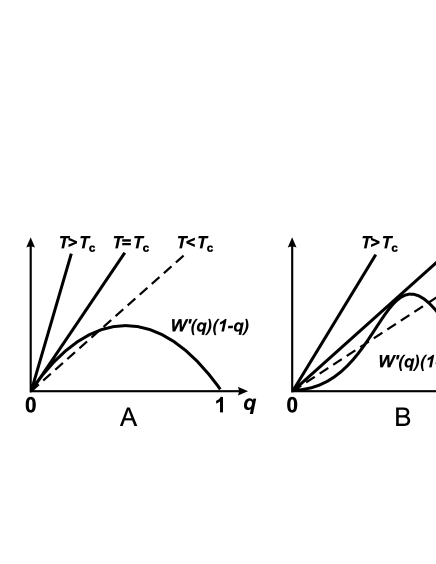
Figure 9: Stability criterium Eq.(57) for $h=0$.  (A): $p=2$  (B): $p>2$. The left hand side is plotted for various temperatures. For $T<T_{c}$ the stability criterium is violated.

Assuming $W(q)\sim q^{p}$ for $q\to 0$ two cases have to be distinguished:

• $p=2$: For $h=0$ a second solution $q_{c}$ branches off for $T<T_{c}$. The stability criterium is, however, violated for $q(t)<q_{c}$. This means that a phase transition into an off equilibrium phase has to take place at $T=T_{c}$. Since this solution branches off continuously from $\overline{q}=0$ at $T_{c}$ this transition is referred to as continuous transition. For $h\neq 0$ the straight line representing the left hand side cuts the $q\!=\!0-$axis at some negative value and there is no transition in finite field [39].

• $p>2$:  For $T\!>\!T_{c}$ again a single solution $\overline{q}=0$ exists. At $T_{c}(h)$ a new solution $q_{c}$ fulfilling

  $$W^{\prime}\big{(}q_{c}\big{)}\,\big{(}1-q_{c}\big{)}/q_{c}=T_{c}$$ (58)

  shows up. This means that the resulting phase transition is discontinuous. For $T=T_{c}$ and $q=q_{c}$ the slope of the left and right hand side of Eq.(57) has to be the same resulting in

  $$T_{c}=W^{\prime\prime}(q_{c})\,(1-q_{c})-W^{\prime}(q_{c}).$$ (59)

  The two Eqs.(58) and (59) determine $T_{c}$ and $q_{c}$.

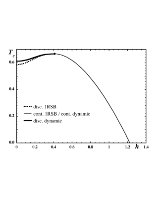
Figure 10: Phase diagram of the spherical $p$-spin interaction spin-glass [22].

This discussion can be extended to $h\neq 0$ [22]. The resulting phase diagram is shown in Fig.10 for the $p=3$-spin-glass with $W(q)=\mbox{$\frac{1}{3!}$}q^{3}$.

For $h<0.41$ the transition is discontinuous. The transition temperatures $T_{c}(h)$ obtained from dynamics is higher than the one found in replica theory. This surprising result might be explained by the proposal that the dominant states counted for in replica theory are not reached by the dynamics investigated [40].

For $h>0.41$ the transition is continuous and both theories give the same transition temperature.

The results of a numerical integration of Eq.(53) for $h=0$ is shown in Fig.11 for temperatures slightly above and at the critical temperature $T_{c}$. The asymptotic behaviour $q(t)$ close to $T_{c}$ can be analysed by identifying appropriate scaling functions for different regions in time and by matching [19, 21, 22]. This resembles very much the crossover scaling analysis near multi critical points [41]. From Fig.11 one can read off two characteristic temperature dependent time scales: A plateau time $\tau_{p}(T)$ can be defined as $q(\tau_{p})=q_{c}$ and a second time scale $\tau_{a}(T)$ characterising the final decay. It may be defined as $q(\tau_{a})=\mbox{$\frac{1}{2}$}q_{c}$.

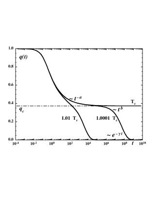
Figure 11: Correlation function $q(t)$ for $T\geq T_{c}$ [22].

For $t\ll\tau_{p}(T)$ the correlation-function approaches some universal function $q(t)\to\hat{q}_{o}(t)$ as $T\to T_{c}$. For $1\ll t\ll\tau_{p}(T)$ Eq.(53) is solved by

$$\hat{q}_{o}(t)\to q_{c}+c_{o}\,t^{-a}.$$ (60)

The dynamical critical exponent $a$ is solution of

$$\frac{\Gamma(1-a)^{2}}{\Gamma(1-2a)}=\frac{(1-q_{c})W^{\prime\prime\prime}(q_{c})}{2\,W^{\prime\prime}(q_{c})}.$$ (61)

This result is obtained by inserting Eq.(60) into Eq.(53) with $T=T_{c}$. For $t\!\to\!\infty$ the leading contribution is ${\cal O}(1)$. The next to leading contributions ${\cal O}(t^{-a})$ yield Eq.(58) and Eq.(59) respectively. Collecting terms ${\cal O}(t^{-2a})$ Eq.(61) is obtained.

The scaling function ansatz for $t\sim\tau_{p}$ is

$$q(t)\approx q_{c}+\tau_{p}^{-a}\hat{q}_{p}(t/\tau_{p}).$$ (62)

The scale factor $\tau_{p}^{-a}$ follows from matching Eq.(60) and Eq.(62) at some $1\ll t\ll\tau_{p}$ and $\hat{q}_{p}(\tau)\to c_{o}\tau^{-a}$ for $\tau\to 0$.

The contributions ${\cal O}(T-T_{c})$ to Eq.(60) for $t\sim\tau_{p}$ give

$$\tau_{p}\sim(T-T_{c})^{-1/2a}.$$ (63)

For $\tau_{p}\ll t\ll\tau_{a}$ Eq.(53) is solved by

$$\hat{q}_{p}(\tau)\to-c_{p}\,\tau^{b}$$ (64)

with $b$ obeying

$$\frac{\Gamma(1+b)^{2}}{\Gamma(1+2b)}=\frac{(1-q_{c})W^{\prime\prime\prime}(q_{c})}{2\,W^{\prime\prime}(q_{c})}=\frac{\Gamma(1-a)^{2}}{\Gamma(1-2a)}.$$ (65)

This means that the two dynamical critical exponents $a$ and $b$ are not independent [19, 22].

The last scaling regime applies for $t\sim\tau_{a}$. The scaling ansatz is

$$q(t)=\hat{q}_{a}(t/\tau_{a}).$$ (66)

Matching to Eq.(62) yields

$$\hat{q}_{a}(\tau)\to q_{c}-c_{p}\,\tau^{b}\quad{\rm for}\quad\tau\to 0$$ (67)

and

$$\tau_{p}=\tau_{a}^{b/(a+b)}$$ (68)

and with Eq.(63)

$$\tau_{a}\sim(T-T_{c})^{-(a+b)/2ab}.$$ (69)

This means that only a single independent critical exponent exists. The scaling functions $\hat{q}_{o}(t)$, $\hat{q}_{p}(\tau)$ and $\hat{q}_{a}(\tau)$ have to be determined numerically.

The imaginary part of the frequency dependent susceptibility is

$$\chi^{\prime\prime}(\omega)=\int_{0}^{\infty}\!\mbox{d}t\,r(t)\,\sin(\omega t)=\beta\,\omega\int_{0}^{\infty}\!\mbox{d}t\,q(t)\,\cos(\omega t)$$ (70)

where the second expression is derived from the FDT, Eq.(37). Near $T_{c}$ the main contributions are due to $t\sim 1$ and $t\sim\tau_{a}$, respectively. Inserting the scaling discussed above

$$\chi^{\prime\prime}(\omega) = \beta\omega\int_{0}^{\infty}\!\mbox{d}t\,q_{0}(t)\,\cos(\omega t)+\beta\mbox{$\frac{\omega}{\omega_{a}}$}\int_{0}^{\infty}\!\mbox{d}\tau\,\hat{q}_{a}(\tau)\,\cos(\mbox{$\frac{\omega}{\omega_{a}}$}\tau)$$ (71)

$$= \chi^{\prime\prime}_{o}(\omega)+\chi_{a}^{\prime\prime}(\mbox{$\frac{\omega}{\omega_{a}}$})$$

with

$$\omega_{a}=1/\tau_{a}\sim(T-T_{c})^{(a+b)/2ab}.$$ (72)

With Eq.(60) for $\omega\to 0$

$$\chi^{\prime\prime}_{o}(\omega)\to\beta c_{o}\Gamma(1-a)\cos(\mbox{$\frac{1}{2}$}\pi(1-a))\,\omega^{a}$$ (73)

is found. For $\omega\ll\omega_{a}$ the second contribution with Eq.(64) gives

$$\chi^{\prime\prime}_{a}(\omega)\to\beta c_{a}\Gamma(1+b)\cos(\mbox{$\frac{1}{2}$}\pi(1+b))\,\omega^{-b}.$$ (74)

Combining both expressions $\chi^{\prime\prime}(\omega)$ shows a minimum at a frequency

$$\omega_{p}\sim\tau_{a}^{b/(a+b)}\sim\tau_{p}^{-1}\sim(T-T_{c})^{1/2a}.$$ (75)

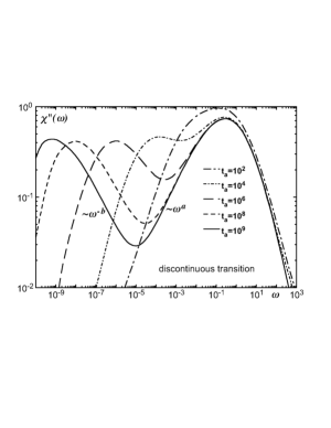
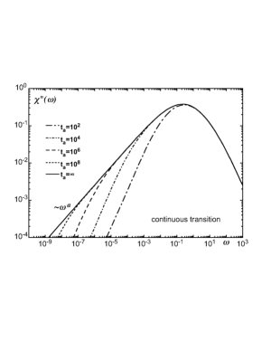
Figure 12: Susceptibility $\chi^{\prime\prime}(\omega)$ computed from the numerical solution of Eq.(53) for $h=0$ and various temperatures characterised by $\tau_{a}(T)$, Eq.(69). For comparison the susceptibility for finite $h$ in the region of continuous transitions is also shown.

The complete susceptibility is plotted in Fig.12. The similarity with the experiments on glasses, shown in Fig.6a, is obvious, and indeed the data on $CKN$ and other glasses have been fitted to the equivalent results of mode coupling theory [19, 23, 24] reproducing the data quite well.

3.7 Off Equilibrium Dynamics and Aging in the QFDT-Phase

The investigation of the dynamics for $T<T_{c}$ requires to specify some long time scale $\tau_{\infty}$, and to consider the limit $\tau_{\infty}\to\infty$ eventually. There have been several proposals for such a time scale:

• For finite systems with $N$ elements the equilibration time $t_{\infty}$ is finite [9]. For large $N$,   $\tau_{\infty}\sim\mbox{e}^{N^{1/3}}$ [42].
  

• Relaxing interactions $\overline{J(t)\,J(t^{\prime})}\sim\mbox{e}^{(t-t^{\prime})/\tau_{\infty}}$ [10].
  

• Slow cooling with $T(t)=(1-t/\tau_{\infty})\,T_{c}$ [22, 43].
  

• Fast cooling, aging, with $\tau_{\infty}=t_{w}$ [44, 45].

In the following we concentrate on aging. The system is rapidly cooled from high temperatures to some $T<T_{c}$ at $t=0$. Alternatively a strong magnetic field could be switched off at $t=0$. The requirement is, that the initial state is not correlated with the disorder.

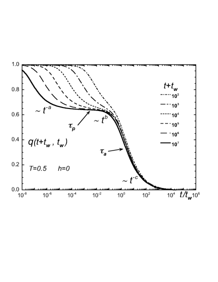
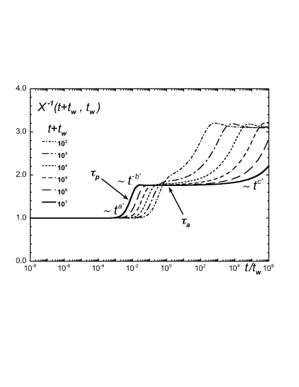
Figure 13: Correlation function $q(t+t_{w},t_{w})$ and FDT-violation $X(t+t_{w},t_{w})$ for $T<T_{c}$ and $h=0$. The curves are plotted for fixed $t+t_{w}$ as functions of $t/t_{w}$. The range $t/t_{w}\sim t+t_{w}$ corresponds to $t_{w}\sim 1$.

Results from a numerical integration [43, 45] of the dynamical mean field equations (47-51) are shown in Fig.13.

Because the system is not in equilibrium at $T<T_{c}\,$, correlation- and response-functions depend on both time variables $t$ and $t^{\prime}$, and not on $t-t^{\prime}$ only as in equilibrium. Furthermore fluctuation dissipation theorems, Eq.(37), are not fulfilled. A measure for FDT-violation is

$$X(t,t^{\prime})=T\frac{r(t,t^{\prime})}{\mbox{$\frac{{\rm d}}{{\rm d}t^{\prime}}$}q(t,t^{\prime})}$$ (76)

which is shown in the lower part of Fig.13. This quantity can be relates to an effective temperature [46]

$$T_{\rm eff}(t,t^{\prime})=X^{-1}(t,t^{\prime})\,T.$$ (77)

For short time $X(t+t_{w},t_{w})\approx 1$ is found. This means that the FDT is fulfilled, while $q(t+t_{w},t_{w})$ decays from 1 to $q_{c}$. A distance in phase space can be defined as

$$D(t,t_{w})=\sqrt{\mbox{$\frac{1}{2}$}\left\langle{\big{(}\varphi_{i}(t+t_{w})-\varphi_{i}(t_{w})\big{)}^{2}}\right\rangle}=\sqrt{\,1-q(t+t_{w},t_{w})\Big{.}\,}.$$ (78)

This distance grows until $q(t+t_{w},t_{w})\approx q_{c}$ is reached, and the resulting $D_{c}=\sqrt{1-q_{c}}$ can be interpreted as the size of a typical valley in phase space. The system apparently equilibrates within such a valley, and escapes only after some characteristic time $\tau_{p}(t_{w})$. This escape is irreversible, which is indicated by the deviation of $X(t+t_{w},t_{w})$ from 1 starting at $t\sim\tau_{p}(t_{w})$.

For $t>\tau_{p}(t_{w})$ the parameter $X(t+t_{w},t_{w})$ reaches a plateau at some $X_{c}$, which extends up to $t\gg t_{w}$. In this regime a modified fluctuation dissipation theorem (QFDT) holds. A solution of this kind was first observed in the context of learning in neural networks exhibiting a discontinuous transition as well [6]. It appears to be a common feature of discontinuous freezing transitions [4, 22].

Investigating the asymptotic behaviour of the solutions of the dynamical mean field equations, Eqs.(47-51), the parameters $q_{c}$, $\overline{q}$, $\overline{\mu}$, $\overline{m}$ and $X_{c}$ can be evaluated analytically [22]. Especially $q_{c}$ is given by $q_{c}=\beta\,W^{\prime}(q_{c})\,(1-q_{c})$, which is of the form of Eq.(58), indicating that the solution is marginally stable at all temperatures $T<T_{c}$.

The crossover scaling analysis is similar to the one discussed for ergodic dynamics in the previous section, but the time scales $\tau_{p}(t_{w})$ and $\tau_{a}(t_{w})$ are now determined by the waiting time$t_{w}$.

Again dynamical critical exponents are introduced. They obey

$$\frac{\Gamma(1-a)^{2}}{\Gamma(1-2a)}=X_{c}\,\frac{\Gamma(1+b)^{2}}{\Gamma(1+2b)}=\frac{(1-q_{c})W^{\prime\prime\prime}(q_{c})}{2\,W^{\prime\prime}(q_{c})}$$ (79)

which is identical to the result Eq.(65) for $T>T_{c}\,$, except for the factor $X_{c}$. The behaviour of $X(t+t_{w},t_{w})$ for $1\ll t\ll\tau_{p}$ and $\tau_{p}\ll t\ll\tau_{a}$, respectively, is also ruled by power laws, as indicated in the lower part of Fig.13. The resulting exponents fulfil [43, 45]

$$a^{\prime}=3a+1\qquad\quad b^{\prime}=3b-1.$$ (80)

Obviously for the existence of the QFDT-phase $b^{\prime}>0$ has to be fulfilled. $b^{\prime}=0$ therefore marks a phase transition from the QFDT-phase ($\cal A$-phase) to a phase with a hierarchy of long time scales ($\cal B$-phase). Another criterium to be fulfilled is $X(t,t^{\prime})\geq 1$. This gives rise to yet another phase ($\cal C$-phase) which covers only a tiny portion of the phase diagram.

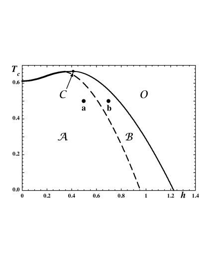
Figure 14: Phase diagram of the spherical $p\!\!=\!\!3-$spin interaction spin-glass [45].   ${\cal O}$: Ergodic phase. ${\cal A}$: QFDT-phase. ${\cal B}$ and ${\cal C}$: Phases with a hierarchy of long time scales. The points a and b are discussed later.

The complete phase diagram is shown in Fig.14. Qualitatively the same phase diagram is found for the mean field model of a particle moving in a correlated random potential [4].

In phase ${\cal A}$ the plateau-time $\tau_{p}$ and the characteristic time scale for aging $\tau_{a}$ are again related by Eq.(68) with the modified relationship, Eq.(79), among the exponents.

For $t\sim t_{w}$ it has been argued [44, 12] that

$$q(t+t_{w},t_{w})=Q\big{(}h(t+t_{w})/h(t_{w})\big{)}$$ (81)

as long as $X(t+t_{w},t_{w})\approx X_{c}$. The function $h(t)$ has to be monotonic, but is otherwise not determined. The arbitrariness in $h(t)$ resembles the invariance postulated for the long time behaviour of the SK-Model [9, 10].

$Q(x)$ can be computed numerically and $Q(x)-q_{c}\sim(x-1)^{b}$ for $x\to 1$. Especially for zero field the exponent $b=1$ and

$$Q(x)=\frac{q_{c}}{x}$$ (82)

is found. The postulate of scaling with $\tau_{a}(t_{w})=t_{w}$ yields $h(t)=t^{c}$. The numerical results [45] shown in Fig.13 agree reasonably well with this form of scaling and in particular with $c\approx 1/2$.

For the analogous case of the drift of a particle in a random potential [4],  $\tau_{a}\sim\tau_{\infty}^{\mu}\,$, with $\mu=1-a(3b-1)/\big{(}2(a+b)+a(3b-1)\big{)}$, has been found in the ${\cal A}$-phase. In this problem the time scale $\tau_{\infty}=1/v_{\rm drift}$ plays the same role as $t_{w}$ for aging. Typical values are $\mu\sim 0.9\cdots 0.95$. Scaling of the form given in Eq.(66) with $\tau_{a}(t_{w})\sim t_{w}^{\mu}$ is obtained from $h(t)=\mbox{e}^{(t^{\eta}-1)\,c/\eta}$ with $\eta=1-\mu$. The numerical solutions [45] indicate $\eta>0$, but the longest time investigated is not long enough, to decide on the actual value of $\eta$.

3.8 Off Equilibrium Dynamics and Aging in the ${\cal B}$-Phase

We now turn to the ${\cal B}$-phase. Fig.15 shows correlation-function $c(t+t_{w},t_{w})=q(t+t_{w},t_{w})-m(t+t_{w})\,m(t_{w})$ and FDT-violation parameter $X(t+t_{w},t_{w})$ for field and temperature values indicated as points a and b in Fig.14. The qualitative difference between ${\cal A}$- and ${\cal B}$-phase is clearly visible.

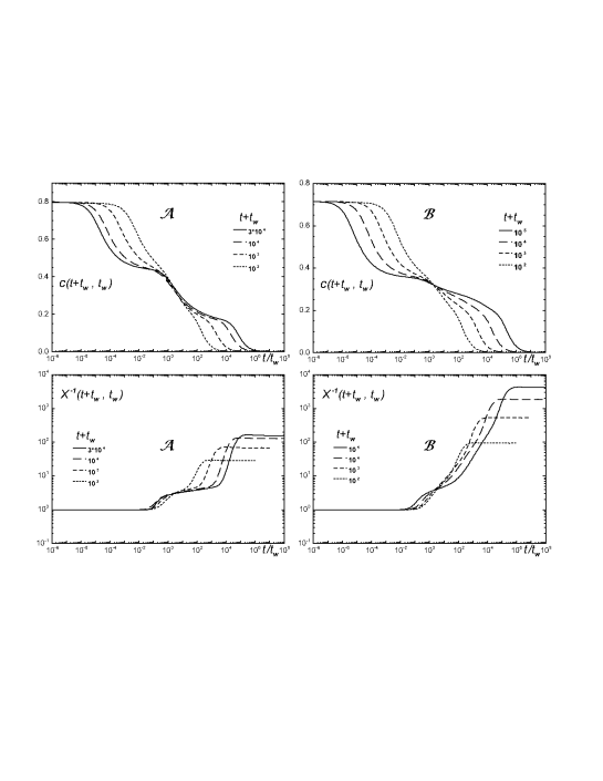
Figure 15: Correlation function $c(t+t_{w},t_{w})=q(t+t_{w},t_{w})-m(t+t_{w})\,m(t_{w})$ and FDT-violation parameter $X(t+t_{w},t_{w})$  for $T=0.5$,  $h=0.5$ (${\cal A}$-phase) and $h=0.7$ (${\cal B}$-phase) [45] corresponding to point a and b in Fig.14. The curves are plotted for fixed $t+t_{w}$. The range $t/t_{w}\sim t+t_{w}$ corresponds to $t_{w}\sim 1$.

In the ${\cal A}$-phase, for $t\gg\tau_{p}$ and $t_{w}\gg 1$, the correlation function approaches a scaling form

$$c(t+t_{w},t_{w})\to\hat{c}_{a}(t/\tau_{a})\qquad{\rm with}\quad\tau_{a}\approx t_{w}\,,$$ (83)

whereas no such scaling is found in the ${\cal B}$-phase. This is in some analogy to one step versus full replica symmetry breaking [8].

Within replica theory the $p\!\!=\!\!3$-spin-glass does, however, not exhibit a full replica symmetry broken phase at all. This is another difference in the phase diagrams obtained from dynamics and replica theory. For the same range of time, the FDT-violation parameter $X(t+t_{w},t_{w})$ develops a plateau in the ${\cal A}$-phase, consistent with the QFDT-solution, whereas no such plateau shows up in the ${\cal B}$-phase.

3.9 Mean Field Dynamics of Systems with Short Ranged Interactions

The slowing down of the dynamics near $T_{c}$ in a disordered system is not expected to be associated with a diverging length scale, at least not on the level considered here. A diverging length scale is expected only for certain four point correlation functions, which are factorized in the dynamic mean field theory or in mode coupling theory, e.g.

$$C(R_{ij},t\!-\!t^{\prime})=\overline{\left\langle{\varphi_{i}(t)\varphi_{j}(t)\varphi_{i}(t^{\prime})\varphi_{j}(t^{\prime})}\right\rangle}^{J}\!-\!\overline{\left\langle{\varphi_{i}(t)\varphi_{i}(t^{\prime})}\right\rangle\left\langle{\varphi_{j}(t)\varphi_{j}(t^{\prime})}\right\rangle}^{J}.$$ (84)

Dynamic mean field equations for short ranged interactions can be derived adopting a factorization property

$$q_{i,j}(t,t^{\prime})=f_{i,j}\cdot q(t,t^{\prime})\qquad\quad r_{i,j}(t,t^{\prime})=f_{i,j}\cdot r(t,t^{\prime}).$$ (85)

The corresponding factorization has been proposed and tested within mode coupling theory for supercooled liquids [19, 13]. The resulting equations for the time dependent parts, $q(t,t^{\prime})$ and $r(t,t^{\prime})$, are of the same form as those derived for mean field models, Eqs.(47-51). The definition of $W(q)$, Eq.(44), has to be modified, taking into account the short range nature of the interactions and the form factors $f_{i,j}$. The crucial assumption is, to neglect four point correlations of the form given above.

It should be mentioned, that a rather different picture, based on a droplet model description, has been developed [47]. Both pictures, mean field models and the droplet model, reproduce certain features of short ranged spin-glasses, and no clear cut evidence in favour or against one of the theories seems to exist at present.

3.10 $p$-Spin-Glass with Relaxing Bonds and Cage Relaxation in Supercooled Liquids

In a supercooled liquid one may distinguish two kinds of motion. Each particle in a sense is surrounded by a cage formed by other particles. Within this cage it may vibrate with amplitudes much smaller than the interparticle spacing. This picture is of course simplified in the sense, that the cage is also vibrating, and each particle is also part of the cage of other particles. It is probably more appropriate to view this motion as a collective localized anharmonic vibration. The second type of motion is a rearrangement of the particles forming the cage, or an escape of a particle from its cage. This type of motion involves jumps over distances of the order of the interparticle spacing, and this is supposed to be an activated process [20, 26].

The mode coupling theory for supercooled glasses [19, 13] deals with density fluctuations, and the resulting equations are identical to those derived for the $p\!=\!3$-spin-glass in equilibrium, Eq.(53). The initial decay of the correlation function towards the plateau (see Fig.11) is usually interpreted as being due to the motion within the cages, whereas the ultimate decay is supposed to result from the escape of a particle from its cage. On the other hand, activated processes are not contained in the standard mode coupling theory. The extended theory [48] captures those processes, and yields a rounding of the singularities found in the ideal mode coupling theory at $T_{c}$. This extended theory is still an equilibrium theory and can not describe aging [25].

In the following I sketch a slightly different picture [45] resulting in identical mode coupling type of equations above $T_{c}$. This formulation allows, however, to deal with off equilibrium properties. It is based on a distinction of the two types of motion described above.

We neglect for a moment the activated process of rearrangement of the cages and consider the anharmonic vibrations only. The position of a particle at time $t$ may be written as

$$\vec{x}_{i}(t)=\vec{R}_{i}+\vec{u}_{i}(t)$$ (86)

where $\vec{u}_{i}(t)$ is the momentary displacement of particle $i$ from its mean position $\vec{R}_{i}$. The configuration of the $\vec{R}_{i}$ can be viewed as inherent state [26]. The dynamics of the displacements $\vec{u}_{i}(t)$ is treated within the selfconsistent anharmonic phonon theory [49], developed originally for quantum crystals or strongly anharmonic crystals at high temperatures. The main idea of this approach is, to replace the harmonic and anharmonic coupling constants by their averages over thermal or quantum fluctuations, e.g.

$$\left\langle{V}\right\rangle_{ij}=\int\!\mbox{d}r\,V^{\prime\prime}(r)\,g_{ij}(r).$$ (87)

$V(r)$ is the pair potential and $g_{ij}(r)$ the static pair correlation function between particles $i$ and $j$. Employing the factorization property Eq.(85) and retaining cubic anharmonicities, one ends up with equations identical to those of the dynamic mean field theory, Eqs.(47-51).

The coupling constants $\left\langle{V}\right\rangle_{i\cdots}$ are calculated for fixed mean positions $\vec{R}_{i}$. These positions are, however, random and the coupling constants are therefore random variables as well. They play the role of the $J_{i\cdots}$ in Eq.(18). Taking into account the activated motion of the $\vec{R}_{i}(t)$, the random couplings $J_{i\cdots}(t)$ now depend on time as well. Under the assumption that they are Gaussian distributed random variables, Eq.(3.1) holds in the modified form

$$\overline{J_{i\cdots}(t)J_{j\cdots}(t^{\prime})}=\mbox{$\frac{1}{p!N^{p/2}}$}\{\delta_{i,j}\cdots+\cdots\}W_{p}G_{J}(t-t^{\prime}).$$ (88)

Since the couplings $J_{\cdots}(t)$ are dynamical variables, corresponding correlation functions have to be introduced

$$\overline{J_{i\cdots}(t)\hat{J}_{j\cdots}(t^{\prime})}=\mbox{$\frac{1}{p!N^{p/2}}$}\{\delta_{i,j}\cdots+\cdots\}W_{p}F_{J}(t-t^{\prime}).$$ (89)

The resulting mean field equations are unchanged, except for the modified memory terms, Eq.(3.5),

$$K(t,t^{\prime}) = W^{\prime\prime}\big{(}q(t,t^{\prime})\big{)}\,G_{J}(t-t^{\prime})\,r(t,t^{\prime})+W^{\prime}\,\big{(}q(t,t^{\prime})\big{)}\,F_{J}(t-t^{\prime})$$

$$M(t,t^{\prime}) = W^{\prime}\,\big{(}q(t,t^{\prime})\big{)}\,G_{J}(t-t^{\prime}).$$ (90)

Assuming an activated process for the cage relaxation,

$$G_{J}(t)=\mbox{e}^{-t/\tau_{\rm cage}}\qquad{\rm and}\qquad F_{J}(t)=\frac{\beta_{J}}{\tau_{\rm cage}}\mbox{e}^{-t/\tau_{\rm cage}}$$ (91)

is chosen.

The choice $\beta_{J}=0$ and $\tau_{\rm cage}\to\infty$ is a realisation of quenched disorder [10]. The results for $t_{w}\gg\tau_{\rm cage}$ are similar to those obtained for aging in Sect.3.7, with $\tau_{\rm cage}$ replacing $t_{w}$. This holds in particular for the algebraic decay of the correlation function $q(t)-q_{c}\sim t^{-a}$.

The situation for $\beta_{J}=\beta$ is quite different. This means that the dynamics of the cages (bonds) can also equilibrate, and that fluctuation-dissipation-theorems hold for $t_{w}\gg\tau_{\rm cage}$. Numerical integration of the dynamic mean field equations yields results shown in Fig.16.

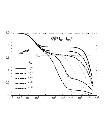
Figure 16: Correlation-function $q(t+t_{w},t_{w})$ for $T<T_{c}$, cage relaxation time $\tau_{\rm cage}=10^{6}$ and various waiting times. For comparison the correlation function for quenched disorder ($\tau_{\rm cage}=\infty$) is also shown (thin lines).

There are now two long time scales, the waiting time $t_{w}$ and the cage relaxation time $\tau_{\rm cage}$. There is yet another characteristic time scale $\hat{\tau}_{\rm cage}=\tau_{p}(\tau_{\rm cage})$ associated with the cage relaxation time, where $\tau_{p}$ is the plateau time introduced in Sect.3.7.

For $t+t_{w}<\hat{\tau}_{\rm cage}$ the results found for quenched disorder are recovered. This means that the approach and departure of the correlation-function from the plateau $q_{c}$ is ruled by power laws, fluctuation-dissipation-theorems are violated for $t>\tau_{p}(t_{w})$ and aging is observed.

For $t_{w}\gg\tau_{\rm cage}$ the system equilibrates, a new plateau value $>q_{c}$ is found. The ultimate decay of the correlation function is now ruled by $\tau_{\rm cage}$. No critical behaviour, i.e. no power laws in $t$, are found. The exponential decay of the correlation function towards the new plateau value is associated with a time scale $\tau_{p}(T)\sim(T_{c}-T)^{-1}$.

Figure 17: Temperature dependent time scales for the $p$-spin-glass with relaxing bonds. For the waiting time $t_{w}$ indicated in the figure the equilibrium and aging regimes are marked

The susceptibility $\chi^{\prime\prime}(\omega)$, calculated for the $p$-spin-glass model with relaxing bonds, depends on the assumptions made for $F_{J}(t)$ or $\beta_{J}$. For equilibrated cage relaxation $\beta_{J}=\beta$ a “knee” shows up at $\omega_{p}\sim 1/\tau_{p}$, and $\chi^{\prime\prime}(\omega)\sim\omega$ for $\omega<\omega_{p}$ whereas $\chi^{\prime\prime}(\omega)\sim\omega^{a}$ for $\omega>\omega_{p}$. Such a knee has actually been observed in CKN [23] but this observation was later withdrawn. The knee is absent assuming non equilibrated cage dynamics with $F_{J}=0$.

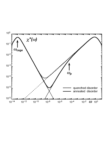
Figure 18: Susceptibility $\chi^{\prime\prime}(\omega)$ for the $p$-spin-glass with relaxing bonds. “Quenched disorder” calculated with $\beta_{J}=0$, “annealed disorder” calculated with $\beta_{J}=\beta$.

It has to be mentioned that the relaxation of the cage configurations has been put in by hand. In particular it is not influenced by the critical slowing down of the anharmonic vibrations. This is a consequence of the mean field model and the $N$-dependent scaling of the interactions, Eq.(20). More realistic models with short range interactions would yield a coupling of the dynamics of the interactions $J$ and the anharmonic vibrations, even within the mean field approximation discussed in Sect.3.9. This has, however, not been worked out.

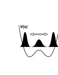
Figure 19: Coupled 1-2-phonon oscillation in an anharmonic potential.

The picture outlined in this section attributes the dynamics of a supercooled liquid, on a time scale shorter than the life-time of cages, to anharmonic vibrations. The instability at $T_{c}$ is attributed to a softening of a coupled oscillation of the center of mass and the width of the thermal cloud, representing the motion of a particle in its cage. This motion is sketched in Fig.19. The idea of a coupled 1-2-phonon process was originally developed for quantum crystals [49]. The critical slowing down near $T_{c}$ within this picture is not directly related to the glass transition, and the actual glass transition at $T_{g}$ has to be attributed to a slowing down of the activated cage relaxation.

The standard interpretation [21, 13, 12] is, to identifying the dynamic transition temperature $T_{c}$ with the crossover region in glasses, and the onset temperature of replica symmetry breaking $T_{\rm RSB}$ with the Kauzmann temperature, which has to be lower than the glass transition temperature $T_{g}$. A comparison of $T_{c}$ and $T_{g}$ for various glass formers, as done in Fig.5, reveals that both temperatures can be rather far apart, whereas model calculations [50] result in differences between $T_{c}$ and $T_{RSB}$ much smaller than the values observed.

4 Outlook

In this lecture I have concentrated on the dynamics of disordered systems treated in mean field theory. I have discussed models within physics but also models for various questions outside physics. Among those are optimization problems, neural networks and problems related to economics. Especially for the applications outside physics, where spacial dimension is not relevant, mean field theory is in many cases exact. The dynamic mean field theory is quite rich because the order parameters are functions of two time variables, the correlation- and response-functions. At high temperature or strong noise level, the systems are ergodic. Lowering the temperature or noise level, a freezing transition shows up and the system becomes non ergodic.

Even on the level of mean field dynamics there are open questions, for instance the arbitrariness in the time parametrization function $h(t)$ discussed in Sect.3.7, or the scaling form of correlation- and response-functions in the aging regime of the ${\cal B}$-phase, discussed in Sect.3.8. A more thorough understanding of the relationship between dynamics and replica theory is desired. In particular there is no obvious prescription of how to calculate entropy or free energy from dynamics. These quantities are, however, of prime interest in replica theory.

The coarse features of aging in spin-glasses are reasonably well described by dynamic mean field theory. There are, however, more elaborate experiments investigating special cooling and heating schedules [17]. It is not clear whether they can be understood on the basis of dynamic mean field theory.

Glasses and spin-glasses are systems with short ranged interactions. Some of their properties are captured by dynamic mean field theory or replica theory. Spacial correlations are not taken into account and questions concerning the existence of diverging length scales can not be answered. On the other hand real space formulations, e.g. the droplet model for spin-glasses [47] or models with kinetically constraint dynamics for glasses [27, 28], are concerned with spacial aspects and a better understanding of discrepancies and common features would be desired.

After all, it is surprising that the dynamic mean field theory for disordered systems can be applied to so many systems in physics and in other disciplines.
Acknowledgment: Partially supported by the ESF-programme SPHINX.

References

-
[1]
K. Binder and A. P. Young, Rev. Mod. Phys. 58, 801 (1986);
K. Fischer and J. Hertz, Spin-glasses, (Cambridge Univ. Press., Cambridge, 1991). -
[2]
M. D. Ediger, C. A. Angell and S. R. Nagel, J. Phys. Chem. 100,13200
(1996);
P. G. Debenedetti and F. R. Stillinger, Nature 410, 259 (2001). -
[3]
Y. G. Sinai, Theor. Probap.Its Appl. 27, 247 (1982);
P. le Doussal and V. M. Vinokur, Physica C, 254, 63 (1995);
S. Scheidl, Z.Physik B 97, 345 (1995);
L. F. Cugliandolo and P. Le Doussal, Phys. Rev. E 53, 152 (1996). - [4] H. Horner, Z. Phys. B 100, 243 (1996).
-
[5]
L. C. E. Struick, Physical Aging in Amorphous Polymers and Other
Materials (Elsevier, Houston, 1978);
E. Vincent, J. Hammann, M. Ocio, J. P. Bouchaud, and L. Cugliandolo, in Complex Behaviour of Glassy Systems, M. Rubi Editor, Lecture Notes in Physics (Springer Verlag, Berlin, 1997), Vol.492, 184. - [6] H. Horner, Z. Phys. B86, 291 (1992) and Z. Phys. B87 371 (1992).
-
[7]
D. Challet and Y-C. Zhang, Physica A 246, 407, (1997);
D. Challet and M. Marsili, Phys. Rev. E 60 R6271 (1999) and cond-mat/9904071
D. Challet, http://www.unifr.ch/econophysics/minority. - [8] M.Mézard, G.Parisi and M.A.Virasoro, it Spin glass theory and beyond, World Scientific (Singapore 1987).
- [9] H. Sompolinsky and A. Zippelius, Phys. Rev. B 25, 6860 (1982).
- [10] H. Horner: Z. Phys. B57, 29 (1984), Z. Phys. B57, 39 (1984) and Z. Phys. B66, 175 (1987).
- [11] J. P. Bouchaud, L. Cugliandolo, J. Kurchan, and M. M ezard, Out of Equilibrium dynamics in spin-glasses and other glassy systems, in ‘Spin-glasses and Random Fields’, A. P. Young Editor, (World Scienti c, Singapore, 1998).
- [12] L. Cugliandolo, Les Houches Lecture Notes 2002, cond-mat/0210312.
- [13] R. Schilling, this Volume.
- [14] S. Nagata et.al., Phys.Rev. B 19, 1633 (1979).
- [15] K. Gunnarson et.al., Phys.Rev. B43, 8199 (1991).
- [16] Ph. Refregier, E. Vincent, J. Hammann and M. Ocio, J.Phys(France) 48,1533 (1987).
- [17] E. Vincent, V. Dupuis, M. Alba, J. Hammann and J.-P. Bouchaud, Europhys. Lett., 29,1 (1999).
- [18] C. A. Angell, Relaxation in Complex System, K. L. Ngai and G. B. Wright (Eds.) (US Dept. Commerce, Spring eld, 1985).
-
[19]
U. Bengtzelius, W. Götze and A. Sjölander, J. Phys. C 17, 5915
(1984);
W. Götze, in Liquids, Freezing and the Glass Transition, eds. J. P. Hansen, D. Levesque and J. Zinn-Justin, North Holland, Amsterdam 1991;
W. Götze and L. Sjögren, Rep. Prog. Phys. 55, 241 (1992). - [20] E. Dont, The Glass Transition, Springer Series in Materials Scienc, Vol 48 (2001).
- [21] T. R. Kirkpatrick and D. Thirumalai, Phys. Rev. Lett. 58, 2091 (1987); Phys. Rev. B 36, 5388 (1987). T. R. Kirkpatrick and P. Wolynes, Phys. Rev. B 36, 8552 (1987).
- [22] A. Crisanti, H. Horner and H-J Sommers, Z.Phys. B 92, 257 (1993).
-
[23]
G. Li, W.M. Du, X.K. Chen, H.Z. Cummins and N.J. Tao, Phys. Rev. A 45,
3867 (1992).
H.C. Barshilia, G. Li, G.Q. Shen and H.Z. Cummins, Phys. Rev. E 59, 5625 (1999). -
[24]
W. Götze and L. Sjögren, Z. Phys. B 65, 415 (1987) and J. Phys. C 21, 3407 (1988).
W. Götze, J. Phys. Condens. Matter, 11, A1 (1999). - [25] B.E. Reed, J.Non-Cryst.Sol. 131, 408 (1991).
-
[26]
F.H. Stillinger and T.A. Weber, Phys. Rev. A 25, 978 (1982);
S. Sastry, P.G. Debenedetti and F. Stillinger, Nature, 393, 554 (1998). - [27] J. Jäckle and S. Eisinger, Z. Phys. B 84, 115 (1991).
- [28] L. Berthier and J.P. Garrahan, Phys. Rev. E 68, 041201 (2003) and cond-mat/0306469.
- [29] H. Kinzelbach and H. Horner, J. Phys. I (France) 3, 1329 (1993) and J. Phys. I (France) 3, 1901 (1993).
-
[30]
J. Hertz, A. Krogh and R.G. Palmer, Introduction to the Theory of Neural
Computation, Addison Wesley (Redwood City (1991).
D.J. Amit, Modeling Brain Function — The World of Attractor Neural Networks, Cambridge University Press (Cambridge 1989). - [31] J.J. Hopfield, Proc.Nat.Acad.Sci. USA, 81, 2554 (1982).
- [32] H. Horner, D. Bormann, M. Frick, H. Kinzelbach and A. Schmidt, Z. Phys. B 76, 381 (1989).
- [33] S. Kirkpatrick, C.D. Gelatt and M.P. Vecchi, Science 220, 671 (1983).
- [34] Y. Fu and P. W. Anderson, J. Phys. A 19, 1605 (1986).
-
[35]
R. Monasson and R. Zecchina, Phys. Rev. Lett. 76, 3881 (1996) and Phys.
Rev. E 56 1357 (1997).
O.C. Martin, R. Monasson and R. Zecchina, Theoretical Computer Science 265 3 (2001) or cond-mat/0104428. - [36] S. F. Edwards and P. W. Anderson, J. Phys. C 5, 965 (1975).
- [37] D. Sherrington and S. Kirkpatrick, Phys. Rev. Lett. 35, 1972 (1975).
- [38] R. Bausch, H.K. Janssen and H. Wagner, Z. Phys. B 24, 97 (1976).
- [39] W. Zippold, R. Kühn and H. Horner, Eur.Phys.J. B 13, 531 (2000).
- [40] A. Barrat, R. Burioni and M. Mezard, J. Phys. A 29, L81 (1996).
-
[41]
I.D. Lawrie and S. Sarbach, Phase Transitions and Critical Phenomena, Vol.
9 C. Domb and J.L. Lebowitz, eds. (Academic, London, 1984).
J.M. Yeomans, Statistical mechanics of phase transitions (Clarendon, Oxford, 1992). - [42] H. Kinzelbach and H. Horner, Z.Phys. B84 (1991).
-
[43]
H. Horner, Europhys. Lett. 2, 487 (1986).
M. Freixa-Pascual and H. Horner, Z. Phys. B80,95 (1990). - [44] L. F. Cugliandolo and J. Kurchan, Phys. Rev. Lett. 71, 173 (1993).
- [45] H. Horner, (to be published).
- [46] L. F. Cugliandolo, J. Kurchan and L. Peliti, Phys. Rev. E55, 3898 (1997).
- [47] D.S. Fisher and D.A. Huse, Phys. Rev. Lett 56, 1601 (1986); Phys. Rev. B 38, 373 (1988).
- [48] M. Fuchs, W. Götze, S. Hildebrand and A. Latz: J. Phys. Cond. Matter 4, 7709 (1992).
- [49] H. Horner, Z. Phys. 205, 72 (1967); and in Lattice Dynamics, Eds. G.K. Horton and A.A.Maradudin (North-Holland , Amsterdam 1972).
- [50] V. Krakoviack and C. Alba-Simionescoy, Europhys. Lett. 51, 420 (2000) and cond-mat/9912223.
Index
- A-phase, 23
- aging, 1, 4, 7, 13, 21
- B-phase, 23, 24
- cage relaxation, 26
- combinatorial optimisation, 1, 9
- continuous transition, 18
- coupled 1-2-phonon process, 30
- creep, 1, 8
- critical exponent, 20, 23
- crossover region, 2
- crossover scaling, 19, 23
- discontinuous transition, 18, 23
- drift of a particle, 8, 23, 24
- droplet model, 26
- dynamic mean field theory, 16
- econophysics, 1, 10
- effective temperature, 22
- ergodic components, 2
- ergodic phase, 17
- factorization property, 27
- FDT-violation, 22, 24
- field cooled susceptibility, 3
- fluctuation-dissipation-theorem, 14, 17
- freezing temperature, 2
- freezing transition, 13
- frustration, 3
- glass transition, 5
- glassy dynamics, 1
- Glauber dynamics, 5, 11
- graph bipartitioning, 9
- Ising model, 4
- K-sat problem, 10
- Langevin dynamics, 13
- marginal stability, 23
- mean field model, 11
- memory terms, 17
- minority game, 10
- mode coupling theory, 2, 6, 21
- neural network, 1, 8, 23
- p-spin-glass, 2, 6, 7, 11, 25, 26, 29
- path integral representation, 13
- phase diagram, 18, 23
- pinning, 1, 8
- plateau, 19, 23
- QFDT, 23, 25
- QFDT-phase, 21, 23
- quenched disorder, 15
- reparametisation invariance, 24
- replica symmetry breaking, 1, 12, 25
- replica theory, 1
- replica trick, 12
- selfconsistent phonon theory, 27
- short ranged interactions, 25
- simulated annealing, 1, 9, 10
- SK-model, 11
- spherical model, 11
- spin-glass, 1, 2
- stability criterium, 18
- supercooled liquid, 1, 5, 26
- susceptibility, 6, 20, 21, 28
- ultrametricity, 2
- waiting time, 1
- zero field cooled susceptibility, 3