”Bloch oscillations” in the Mott-insulator regime

Abstract

We study the dynamical response of cold interacting atoms in the Mott insulator phase to a static force. As shown in the experiment by M. Greiner et. al., Nature 415, 39 (2002), this response has resonant character, with the main resonance defined by coincidence of Stark energy and on-site interaction energy. We analyse the dynamics of the atomic momentum distribution, which is the quantity measured in the experiment, for near resonant forcing. The momentum distribution is shown to develop a recurring interference pattern, with a recurrence time which we define in the paper.

1. Introduction. Recently much attention has been paid to the properties of Bose-Einstein condensates of cold atoms loaded into optical lattices. In particular, the experimental observation of the superfluid (SF) to Mott insulator (MI) transition Grei02 has caused a great deal of excitement in the field. Note, that besides demonstrating the SF-MI quantum phase transition, the same experiment also rose the problem of the system’s response to a static force (used in the experiment to probe the system). Obviously, the response depends on whether the atoms are initially prepared in the SF state or the MI state. The former case was investigated theoretically in recent papers prl ; preprint ; pre (see also related studies Berg98 ; Choi99 ; Chio00 ). It was found that, similar to the case of non-interacting atoms, the static force induces Bloch oscillations of the atoms which, however, may be affected rather dramatically by the presence of atom-atom interactions. The latter case of MI initial state was analysed in Ref. Brau02 ; Sach02 , and is also the subject of the present Brief Report. In particular, we address the evolution of the atomic momentum distribution not discussed so far. We show that, in formal analogy with usual Bloch oscillations, a static force causes oscillations of the atomic momentum, however, with a different characteristic frequency.

2. The model and numerical approach. Like in our earlier studies prl ; preprint ; pre , we model cold atoms loaded into an optical lattice by the Bose-Hubbard Hamiltonian, with an additional Stark term:

$$\widehat{H} = -\frac{J}{2}\left(\sum_{l}\hat{a}^{\dagger}_{l+1}\hat{a}_{l}+h.c.\right)$$ (1)

$$+\frac{W}{2}\sum_{l}\hat{n}_{l}(\hat{n_{l}}-1)+dF\sum_{l}l\hat{n}_{l}\;.$$

In Eq. (1) $J$ is the hopping matrix element, $W$ the on-site interaction energy, $d$ the lattice period, and $F$ the magnitude of the static force. Throughout the paper we consider a one-dimensional lattice and assume, for simplicity, that the filling factor (number of atoms per lattice site) equals unity. Then, the assumption of a Mott-insulator initial state implies $J<0.17W$. In what follows, however, we shall be mainly interested in the limiting case $J\ll W$. Under this condition, the excitation of the system is only possible if the Stark energy is approximately equal to the interaction energy. Indeed, for $dF\cong W$ the atoms may resonantly tunnel in the neighbouring well, thus forming ‘dipole’ (in the terminology of Ref. Sach02 ) states (see Fig. 1).

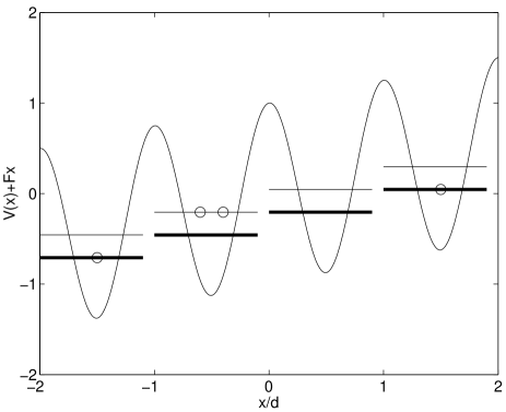
Figure 1: Schematic presentation of the dipole state. Provided the Stark energy (mismatch between the ‘bold levels’ in the figure) is equal to the interaction energy (distance between the ‘bold’ and ‘thick’ levels) the atom may resonantly tunnel in a neighbouring well, thus creating particle-hole excitations of the MI state.

The first step of our analysis is to identify the resonant subspace in the system’s Hilbert space (spanned by Fock states), i.e. the manifold of states resonantly coupled to the MI state. For example, for a finite lattice with $L=8$ and $F>0$, the MI state $|11111111\rangle$ is coupled to the one-dipole states $|20111111\rangle$, $|12011111\rangle$, etc., which are coupled to two-dipole states $|20201111\rangle$, $|20120111\rangle$, etc., which in turn are coupled to three-dipole states, and so on. If $J\ll W$, one actually can neglect the other (non-resonant) states when considering the excitation of the system. The validity of this resonant approximation is illustrated in the upper panel of Fig. 2, where we compare the time evolution of the mean atomic momentum, calculated by using the complete basis (for chosen $L=8$ the total dimension of Hilbert space is ${\cal N}=6435$), and restricted to the resonant manifold respectively (${\cal N}_{R}=47$). It is seen that the resonant approximation works pretty well already for $J/W\cong 0.05$. It is also worth noting that, in the resonant approximation and after scaling time $t\rightarrow Jt/\hbar$, the only relevant parameter of the system is the dimensionless detuning

$$\lambda=(W-dF)/J\;.$$ (2)

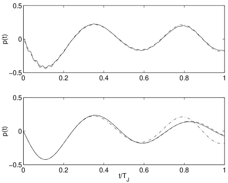
Figure 2: Upper panel: Dynamics of the normalised mean momentum ($p(t)\rightarrow p(t)/JN$) for $L=N=8$, $W=0.0324$, $dF=W$, and $J=0.0019$. The solid line shows the exact dynamics, dashed line corresponds to the resonant approximation. Time axis is scaled with respect to $T_{J}=2\pi\hbar/J$, which is the characteristic time-scale of the system. Lower panel: Dynamics of the mean momentum calculated within the resonant approximation for different system sizes – $L=8$ (dot-dashed line), $L=12$ (dashed line), and $L=16$ (solid line). It is seen that, for the considered time interval $t\leq T_{J}$, convergence towards the thermodynamic limit is reached already for $L=12$.

Let us briefly comment on our choice of periodic (cyclic) boundary conditions used throughout this paper. These are imposed on (1) after a gauge transformation which leads to the time-dependent Hamiltonian

$$\widehat{H}(t)=-\frac{J}{2}\left(e^{i\omega_{B}t}\sum_{l}\hat{a}^{\dagger}_{l+1}\hat{a}_{l}+h.c.\right)+\frac{W}{2}\sum_{l}\hat{n}_{l}(\hat{n_{l}}-1)\;,$$ (3)

with $\omega_{B}=dF/\hbar$ the Bloch frequency. Note that for periodic boundary conditions the quasimomentum is a conserved quantity and, hence, the dipole states can be excited only in coherent superpositions, with the same quasimomentum $\kappa=0$ as for the initial MI state. In particular, for one-dipole excitations this constraint defines the state

$$|D(1)\rangle=\frac{1}{\sqrt{L}}\sum_{l=1}^{L}\widehat{S}^{l}|2011\ldots 11\rangle\;,$$ (4)

where $\widehat{S}$ denotes cyclic permutations: $\widehat{S}|2011\ldots 11\rangle=|1201\ldots 11\rangle$. It is worth noting that for two-dipole (three-dipole, etc.) excitations there are many different states $|D(2)\rangle$, not related to each other by cyclic permutation. In what follows, we refer to the states $|D(m)\rangle$ as the translationally invariant dipole states.

We conclude this section by a remark on the thermodynamic limit $L\rightarrow\infty$. Obviously, the dynamics of a system of finite size differs from the one of an infinite system. However, this difference emerges only after a finite ‘correspondence’ time. This is illustrated in the lower panel of Fig. 2, which shows the mean momentum $p(t)$ for different lattice size $L=8,12,16$. It is seen that an increase of the system size above $L=12$ does not change the result and, hence, for the considered time interval $t\leq T_{J}$ convergence of thermodynamic limit has been reached.

3.Results of numerical simulations. This section reports the results of numerical simulations the system dynamics obtained within resonant approximation. In our numerical simulations we followed the scheme of present-days laboratory experiments, where one measures the momentum distribution of the atoms by using the ‘free-flight’ technique. Precisely, after preparation of the initial state (cooling stage), the atoms are subject to a static force for a given time interval $t$ (evolution stage). Then the static field, as well as the optical potential, is abruptly switched off and the atoms move in free space. Finally, the spatial distribution of the atoms is measured, which carries information about the momentum distribution at the end of the evolution stage. Repeating the experiment for different time intervals $t$, one recovers the time-evolution of the momentum distribution $P(p,t)$.

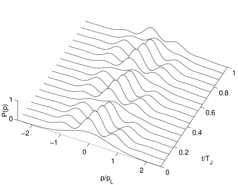
Figure 3: Static force induced dynamics of the atomic momentum distribution for cold atoms in a one-dimensional optical lattice. The depth of optical the potential is 22 recoil energies, the dimensionless detuning $\lambda=2.084$. A periodic change of the distribution is clearly observed. Feeble oscillations of the distribution are an artifact, due to the finite system size ($L=16$).

Figure 3 shows the time-evolution of the atomic momentum distribution for an optical potential depth $v$ equal to 22 recoil energies, and a static force strength $F$ corresponding to $\lambda=2.084$. Note that the $v$ uniquely defines the hopping matrix element $J$ ($J=0.0038$ recoil energies, for $v=22$) and, hence, the tunnelling time $T_{J}=2\pi\hbar/J$. The amplitude $v$ also defines explicite form of the Wannier states $\psi_{l}(x)=\psi_{0}(x-dl)$ and, thus, the initial distribution $P_{0}(p)=P(p,t=0)$ of the atomic momenta. Indeed, since the initial state is MI state, $|\Psi(t=0)\rangle=|D(0)\rangle\equiv|11\ldots 11\rangle$, the momentum distribution at $t=0$ is simply the squared Fourier transform of the Wannier state, as can be easily derived from the definition of the one-particle density matrix remark1 :

$$\rho(x,x^{\prime}) = \sum_{l,m}\rho_{l,m}(t)\psi_{l}(x)\psi_{m}(x^{\prime})$$ (5)

$$\rho_{l,m}(t) = \langle\Psi(t)|\hat{a}^{\dagger}_{l}\hat{a}_{m}|\Psi(t)\rangle\;.$$ (6)

As time evolves, the momentum distribution repeatedly develops a fringe-like interference pattern. More formally,

$$P(p,t)=P_{0}(k)f(p,t)\;,$$ (7)

where $f(p,t)=f(p+p_{L},t)$ is a periodic function of the momentum with the period $p_{L}=2\pi\hbar/d$ defined by the inverse lattice period. For currently considered case $\lambda=2.084$, the function (7) is also (almost) periodic in time with the period $T_{\lambda}\approx 0.33T_{J}$. Note, however, that $f(p,t)$ is in general not periodic (or quasiperiodic) in time, although some characteristic time scale prevails. This statement is illustrated by the upper panel of Fig. 4, where the temporal behaviour of the mean momentum is displayed for different values of the detuning $\lambda$. One clearly observes the decaying oscillations of the mean momentum, where both the period of oscillations and the decay rate increase as the detuning is decreased.

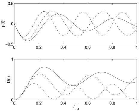
Figure 4: Mean atomic momentum (upper panel) compared to the average number of dipole states (lower panel), as the functions of time, for different values of the detuning $\lambda=0$ (solid line), $1.042$ (dashed line), and $2.084$ (dot-dashed line).

4.Quasienergy spectrum approach. From the point of view of Quantum Optics, momentum oscillations of cold atoms is a process of subsequent excitations of the translationally invariant dipole states $|D(0)\rangle\leftrightarrow|D(1)\rangle\leftrightarrow\{|D(2)\rangle\}\leftrightarrow\ldots$. As an overall characteristic of this process we consider the mean number of dipole states

$$D(t)=-\frac{2}{L}\sum_{m=0}^{L/2}\sum_{j}m|c_{m,j}(t)|^{2}\;,$$ (8)

where the $|c_{m,j}(t)|^{2}$ are occupation probabilities for different dipole states. (Note that $D(t)\leq 1$, due to the chosen normalisation.) The dynamics of $D(t)$ for three different values of the detuning $\lambda$ is shown in the lower panel of Fig. 4. A strong correlation between the number of excited dipole states and oscillations of the mean momentum is clearly observed.

The above results of our numerical simulations can be qualitatively understood by analysing the quasienergy spectrum of the system. An explicite form of the effective Hamiltonian, who’s eigenvalues define the quasienergy spectrum, immediately follows from (3) by employing the resonant approximation and is given in Ref. Sach02 . Namely, using the notion of dipole creation operator $\hat{d}^{\dagger}_{l}=(1/\sqrt{2})\hat{a}^{\dagger}_{l-1}\hat{a}_{l}$ ( which creates a ‘hole’ at site $l$ and a ‘quasiparticle’ at site $l-1$) the effective Hamiltonian reads

$$\widehat{H}_{eff}=\lambda\sum_{l}\hat{d}^{\dagger}_{l}\hat{d}_{l}-\frac{1}{\sqrt{2}}\sum_{l}\left(\hat{d}^{\dagger}_{l}+\hat{d}_{l}\right)\;,$$ (9)

with the constraint that neither there can be more than one dipole at one site ($\hat{d}^{\dagger}_{l}\hat{d}_{l}\leq 1$), nor two dipoles at neighbouring sites (hard core repulsion). As noticed in Ref. Sach02 , the eigenvalue problem for the Hamiltonian (9) can be mapped to the energy spectrum problem for a 1D chain of interacting spins, where a number of analytical results is known. In particular, there is an Ising quantum critical point at $\lambda_{c}=-1.850$, with qualitatively different ground state of the spin system below and above this value of $\lambda$. It should be noted, however, that in the context of our present problem (dynamical response of the system), the eigenvalue problem for the effective Hamiltonian (9) defines the quasienergy spectrum, where the notion of the ground state has no physical meaning.

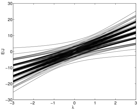
Figure 5: Evolution of the spectrum of effective Hamiltonian (9) under variation of the dimensionless detuning $\lambda$. (Lattice size $L=16$.)

To understand the characteristic structure of the quasienergy spectrum it is convenient to discuss it first for finite $L$. The result of a direct numerical diagonalisation of $\widehat{H}_{eff}$ for $L=16$ is presented in Fig. 5. This figure shows the position of the quasienergy levels, as a function of the dimensionless detuning $\lambda$. To avoid possible confusion with a similar figure in Ref. Sach02 , we note that here only the states of the same translational symmetry as the MI state (i.e., the states with zero value of the quasimomentum) are shown. It is also worth mentioning that the spectrum has reflection symmetry and, hence, when discussing the dynamics (rather than thermodynamics), only the case $\lambda\geq 0$ needs to be considered.

Let us discuss the quasienergy spectrum in more detail. It is convenient to start with large positive $\lambda$. For a large $\lambda$ the spectrum consists of separate levels (or bunches of levels), which in the formal limit $\lambda\rightarrow\infty$ can be associated with the dipole states (or family of dipole states) $|D(m)\rangle$ with given $m$ ($m\leq L/2$). The lowest level in Fig. 5 is obviously the MI state, the level above the one-dipole state $|D(1)\rangle$, followed by the family of states $|D(2)\rangle$, etc. (For negative $\lambda$ the situation is reversed and the MI state $|D(0)\rangle$ is associated with the most upper level.) The key feature of the spectrum is the finite gap $\Delta$ between the quasienergy level $|D(0)\rangle$ and the rest of the spectrum, exiting for arbitrary values of $\lambda$. It is precisely this gap, what defines the characteristic frequency of atomic oscillations seen in Fig. 4. In the thermodynamic limit we have $\Delta\approx 1.43$ for $\lambda=0$ and $\Delta\rightarrow|\lambda|$ for $|\lambda|\rightarrow\infty$ remark2 . Let us also note that in the thermodynamic limit and for $\lambda\approx 0$ the remainder of the quasienergy spectrum is continuous and gapless. This explains an irreversible decay of oscillations, although the decay rate (and its $\lambda$-dependence) remains an open problem.

5.Conclusion. We considered the response of the Mott-insulator phase of cold atoms in an optical lattice to a ‘resonant’ static force. Here the term ‘resonant’ means that the Stark energy $dF$ approximately coincides with on-site interaction energy $W$. Under this condition, the atoms can tunnel in the neighbouring wells of the optical potential, thus creating particle-hole excitations of the Mott-insulator state (the ‘dipole states’). This process directly affects the atomic momentum distribution, which is usually measured in laboratory experiments. Namely, the momentum distribution repeatedly develops an interference pattern with a characteristic period $T_{\lambda}$. This period is uniquely defined by the tunnelling time $T_{J}=2\pi\hbar/J$ ($J$ is the hopping matrix element) and the energy gap between two lowest quasienergy levels, which, in turn, is a unique function of the dimensionless detuning $\lambda=(W-dF)/J$. In particular, for $\lambda=0$, one has $T_{\lambda}\approx 0.67T_{J}$, what, for e.g., for sodium atoms ($E_{R}/\hbar=2\pi\times 8.9$ kHz) in optical potential of 22 recoil energies ($J/E_{R}=0.0038$) corresponds to approx. 20 milliseconds.

References

- (1) M. Greiner, O. Mandel, T. Esslinger, T. W.Hänsch, and I. Bloch, Nature 415, 39 (2002).
- (2) A. R. Kolovsky, Phys. Rev. Lett., 90, 213002 (2003).
- (3) A. Buchleitner and A. R. Kolovsky, Phys. Rev. Lett. (2003); e-print cond-mat/0305037.
- (4) A. R. Kolovsky and A. Buchleitner, Phys. Rev. E 68 0562XX (2003).
- (5) K. Berg-Sorensen and K. Molmer, Phys. Rev. A 58, 1480 (1998).
- (6) D. I. Choi and Q. Niu, Phys. Rev. Lett. 82, 2022 (1999).
- (7) M. L. Chiofalo, M. Polini, and M. P. Tosi, Eur. Phys. J. D 11, 371 (2000).
- (8) K. Braun-Munzinger, J. A. Dunningham, and K. Burnett, e-print cond-mat/0211701.
- (9) Subir Sachdev, K. Sengupta, and S. M. Girvin, Phys. Rev. B 66, 0751128 (2002).
- (10) Note, by passing, that due to translational invariance of the problem, the density matrix is a cyclic matrix (i.e. the rows of the matrix are related to each other by cyclic permutation).
- (11) Note that the limit of large should be considered with precaution because it can violate the resonant approximation.