Landau-Zener transitions in a multilevel system. An exact result.

Abstract

We study the S-matrix for the transitions at an avoided crossing of several energy levels, which is a multilevel generalization of the Landau-Zener problem. We demonstrate that, by extending the Schrödinger evolution to complex time, one can obtain an exact answer for some of the transition amplitudes. Similar to the Landau-Zener case, our result covers both the adiabatic regime (slow evolution.) and the diabatic regime (fast evolution). The form of the exact transition amplitude coincides with that obtained in a sequential pairwise level crossing approximation, in accord with the conjecture of Brundobler and Elser [10].

Landau-Zener (LZ) transitions [1, 2] between two energy states at an avoided level crossing is one of the few exactly solvable problems of time-dependent quantum evolution. The LZ theory has found many applications, and is used to describe a variety of physical systems, ranging from atomic and molecular physics [3], to mesoscopic physics [4].

However, since most of the problems of interest involve more than two energy levels, with transitions between several levels happening simultaneously, it is desirable to extend the LZ theory to multilevel problems. A number of interesting generalizations of the LZ problem have been proposed, in which several energy levels cross at the same time. In some cases, including the so-called bow-tie model [5, 6, 7], the high spin model [8], one can construct an analytic solution. The solutions [5, 6, 7, 8] rely on a special form of the coupling Hamiltonian or on its symmetry, which preserves the integrability of the problem. One of the most efficient methods proposed to treat the generalized LZ problems is the contour integration approach [9].

Much less is known about the general multilevel LZ problem, defined by a time-dependent Hamiltonian of the form

$${\cal H}(t)=\hat{\Delta}+\hat{\nu}t$$ (1)

were $\hat{\Delta}$, $\hat{\nu}$ are hermitian matrices $n\times n$ of a general form. In this problem, one is interested in the evolution

$$i\frac{\partial\psi}{\partial t}={\cal H}(t)\psi$$ (2)

from large negative to large positive times. Since $\hat{\nu}t$ is the leading term in the Hamiltonian at large $t$, it is natural to analyze the evolution in terms of an S-matrix in the basis of states that diagonalize $\hat{\nu}$.

One can construct an approximate solution in the ‘weak coupling’ limit, when the off-diagonal elements of $\hat{\Delta}$ are weak compared to the diagonal ones, $|\Delta_{ij}|\ll|\Delta_{ii}|$, ($i\neq j$). Since in this case the anticrossing gaps of the adiabatic levels (which sometimes are also called ‘frozen levels’) are much smaller than the level separation, the weak coupling regime can be analyzed in a sequential two-level LZ approximation [10], similar to the energy diffusion problem in mesoscopic systems [4].

Brundobler and Elser have noticed [10] that the formula for certain diagonal elements of the S-matrix obtained in such an approximation remains numerically very accurate even at strong coupling, when this approximation supposedly breaks down. This surprising observation, based on a computer simulation of the problem (2),(1), has led Brundobler and Elser to a conjecture that the sequential LZ approximation can in some cases give an exact result.

Below we show that this conjecture is indeed correct. We shall use the method of continuing the Schrödinger evolution (2) to complex time, and matching the $t\to\pm\infty$ asymptotics of the evolving state $\psi(t)$. Our method gives exact results only for some of the transition amplitudes, corresponding to the transitions $|1\rangle_{t=-\infty}\to|1\rangle_{t=+\infty}$, $|n\rangle_{t=-\infty}\to|n\rangle_{t=+\infty}$.

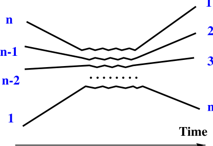
FIG. 1.: Time evolution of the adiabatic (frozen) energy levels of the Hamiltonian (1). The transitions analyzed in this work are $|1\rangle_{t=-\infty}\to|1\rangle_{t=+\infty}$ and $|n\rangle_{t=-\infty}\to|n\rangle_{t=+\infty}$.

It is convenient to analyze the problem in the basis of states that diagonalize $\hat{\nu}$:

$$\hat{\nu}=\left(\begin{array}[]{cccc}\nu_{1}\\ &\nu_{2}\\ &&\ddots\\ &&&\nu_{n}\end{array}\right)\,.$$ (3)

This basis is not the basis of adiabatic states, however, for $t\to\pm\infty$ those states coincide with the adiabatic states, up to permutation. It is also convenient to order the eigenvalues $\nu_{i}$ so that

$$\nu_{1}<\nu_{2}<{\ldots}<\nu_{n}\,.$$ (4)

For simplicity, we assume that the eigenvalues are non-degenerate: $\nu_{i}\neq\nu_{j}$ for $i\neq j$.

To produce a full solution of the Landau–Zener problem completely, one would have to find the transition amplitudes between all different states, or, in other words, to find the scattering matrix $S$, relating the initial state of the system at $t=-\infty$ and the final state at $t=+\infty$:

$$\psi(t=+\infty)=\hat{S}\psi(t=-\infty)\,.$$ (5)

The Landau-Zener theory provides an analytic solution of this problem for $n=2$. Presently, it is not known whether a generalization of this solution exists for $n>2$.

Here, I will pursue a less ambitious goal. I will show how one can obtain the two transition amplitudes $S_{11}$ and $S_{nn}$. In our ‘$\nu$-ordered’ basis notation, this corresponds to the transitions between the lowest and the highest adiabatic energy state: $S_{1\to 1}=S_{A1\to An}$, and $S_{n\to n}=S_{An\to A1}$, where $Ai$ are adiabatic states ordered by their energies (see Fig. 1).

To compute these transition probabilities, I consider the $n$-component state vector $\psi(t)$ at large times $t\to\pm\infty$. At these times, the Hamiltonian is almost diagonal, and the transitions between different adiabatic states are negligible. Therefore, the state $i$’th component $\psi_{i}(t)$ evolves as

$$\psi_{i}(t\to-\infty) = a_{i}e^{-i\phi_{i}(t)}\,,$$ (6)

$$\psi_{i}(t\to+\infty) = b_{i}e^{-i\phi_{i}(t)}\,.$$ (7)

Let us consider the phase $\phi_{i}(t)={\rm arg}\,\psi_{i}(t)$. In the zero-order approximation, when one completely neglects the off-diagonal part $\hat{\Delta}$, the phase is entirely due to $\nu_{i}$:

$$\phi_{i}^{(0)}(t)=\frac{\nu_{i}t^{2}}{2}\,.$$ (8)

To find the phase $\phi_{i}$ more accurately, one notes that in the adiabatic approximation this phase is actually given by an integral of a ‘frozen eigenvalue’ of $\varepsilon_{i}(t)$ the Hamiltonian (1):

$$\phi_{i}(t)=\int\limits^{t}\varepsilon_{i}(t^{\prime})\,dt^{\prime}\,.$$ (9)

At large $t$, $\nu t\gg\Delta$, the eigenvalue $\varepsilon_{i}(t)$ can be found from perturbation theory in $\hat{\Delta}$. To the second order in $\hat{\Delta}$, it is given by

$$\varepsilon_{i}^{(2)}(t)=\nu_{i}t+\Delta_{ii}+\sum_{j\neq i}\frac{|\Delta_{ij}|^{2}}{(\nu_{i}-\nu_{j})t}\,.$$ (10)

Therefore, at large $t$, the phase $\phi_{i}(t)$ can expressed as

$$\phi_{i}(t)=\frac{\nu_{i}t^{2}}{2}+\Delta_{ii}t+\alpha_{i}\ln t+O(\hat{\Delta}^{3})\,,$$ (11)

where

$$\alpha_{i}=\sum_{j\neq i}\frac{|\Delta_{ij}|^{2}}{\nu_{i}-\nu_{j}}\,.$$ (12)

The key observation underlying our approach is that the terms retained in the expansion (11) are the only terms that grow indefinitely at $t\to\infty$. The higher-order terms in $\hat{\Delta}$, written symbolically as $O(\hat{\Delta}^{3})$, remain finite at large $t$.

The asymptotic form of $\psi_{i}(t)$, defined by the expressions (6), (11) and (12), allows one to compute the transition amplitudes $S_{11}$ and $S_{nn}$ as follows [12]. Let us consider the solution (6) for arbitrary complex times $t$, allowing the phase variable $\phi_{i}(t)$ to be complex. Suppose that initially the system is in $k$’th state, so that $a_{i}=0$ for all $i\neq k$, and $a_{k}=1$. At $t\to+\infty$, the system is, in general, described by all $b_{i}\neq 0$. One can try to continue the solution at $t\to+\infty$ to $t\to-\infty$ along one of the two large half-circles, $t=Re^{i\theta}$:
(a) in the upper half-plane, $\theta\in[0,\pi]$, and
(b) in the lower half-plane, $\theta\in[0,-\pi]$.
The contour radius $R$ is assumed to be very large.

FIG. 2.: The contours in the complex time plane used for analytic continuation and asymptotics matching of the solution for the $i=1,n$ components.

When the state $\psi(t)$ is continued analytically along such a contour, its different components will behave differently: some of them increasing, while others decreasing as a function of $|t|$. Indeed, the leading term in $\phi_{i}(t)$ gives for the $i$’th component

$$\psi_{i}\propto\exp\left(\frac{\nu_{i}R^{2}}{2}\sin 2\theta+\frac{i\nu_{i}R^{2}}{2}\cos 2\theta\right)\,.$$ (13)

In matching the asymptotic expansions only the most rapidly increasing terms the wave function must be retained. (For a discussion of this issue in depth, see [11, 12].) For the contour (a) the leading term is given by the $i=n$ component, while for (b) it is the $i=1$ component. Because of that, only $n$’th and $1$’st components of the state $\psi(t\to-\infty)$ can be determined in this way. Without loss of generality, I will consider the $i=1$ case, i.e., perform continuation along the contour (b).

The wave function after continuing along the contour can be found by changing the argument of $t$ as

$$t\to te^{-i\pi}$$ (14)

in Eq. (11). The first and the second term contribute only to the phase of $\psi_{i}(t)$, while the third term changes its modulus:

$$\psi_{1}^{(b)}(t\to-\infty)=b_{1}e^{-\pi\alpha_{1}}e^{-i\frac{1}{2}\nu_{1}t^{2}-i\Delta_{11}t-i\alpha_{1}\ln t}\,.$$ (15)

On the other hand, we assume that this state evolved from the state which initially had only one nonzero component, $|\psi_{i}(t)|=1$, $\psi_{j\neq i}=0$. The time dependence of this component, $\psi_{i}(t)\propto e^{-i\phi_{i}(t)}$, with unit modulus and the phase given Eq. (11), yields

$$\psi_{1}(t\to-\infty)=\exp\left(-{\textstyle\frac{i}{2}}\nu_{1}t^{2}-i\Delta_{11}t-i\alpha_{1}\ln t\right)\,.$$ (16)

Comparing these two expressions, we obtain

$$b_{1}=\exp\left(\pi\alpha_{1}\right)\,,$$ (17)

which gives the transition amplitude of the form

$$S_{1\to 1}=b_{1}=\exp(\pi\alpha_{1})=\exp\left(-\pi\sum_{j\neq 1}\frac{|\Delta_{i1}|^{2}}{\nu_{j}-\nu_{1}}\right)\,.$$ (18)

Similarly, for the $i=n$ component, after going through analytical continuation over the contour (a), we obtain

$$S_{n\to n}=\exp(-\pi\alpha_{n})=\exp\left(-\pi\sum_{j\neq n}\frac{|\Delta_{in}|^{2}}{\nu_{n}-\nu_{j}}\right)\,.$$ (19)

The resulting expressions for the transition amplitude, Eqs. (18),(19), bear similarity with the Landau-Zener formula and, in fact, coincide with it in the $n=2$ case. Just like in the LZ problem, the dependence on the coupling matrix $\hat{\Delta}$ and on the ’rapidity’ $\hat{\nu}$ is such that $S\to 0$ in the adiabatic limit of slow evolution (small $\hat{\nu}$), and $S\to 1$ when the evolution is fast (large $\hat{\nu}$).

Eqs. (18) and (19) coincide with the transition amplitude found by Brundobler and Elser [10] in the sequential pairwise LZ level crossing approximation, and thus prove their conjecture.

The existence of an analytic result for two transition amplitudes may indicate that the entire $S$-matrix could be obtained analytically. It does not seem, however, that a trivial generalization of the above approach will be sufficient for that. We were not able to perform analytic continuation keeping track of the subleading terms, which probably indicates that this is not an optimal method of treating such a problem.

It is of course not unconceivable, in principle, that only two transition amplitudes out of total $n^{2}$ can be obtained in a closed form, while others cannot. However, to the best of the author’s knowledge, there are no other examples known where only a subset of the $S$-matrix is calculable, and thus such a possibility does not seem likely. The author hopes that this paper will stimulate further work towards a more complete understanding of multilevel Landau-Zener transitions.

REFERENCES

- [1] L. D. Landau, Physik Z. Sowjetunion 2, 46 (1932)
- [2] C. Zener, Proc. Roy. Soc. Lond. A 137, 696 (1932)
- [3] H. Nakamura, Nonadiabatic transitions. Concepts, Basic Theories and Applications, (World Scientific, 2002)
- [4] E. J. Austin and M. Wilkinson, J. Phys.: Condens. Matter, 5, 8461-8484, (1993); M. Wilkinson and E. J. Austin, J. Phys.: Condens. Matter, 6, 4153-4166, (1994).
- [5] V. N. Ostrovsky and H. Nakamura, J. Phys. A. 30, 6939 (1997)
- [6] Y. N. Demkov, V. N. Ostrovsky, Phys. Rev. A61 (3), 032705 (2000)
- [7] Y. N. Demkov, V. N. Ostrovsky, J. Phys. B: At. Mol. Opt. Phys. 34, 2419, (2001)
- [8] V. L. Pokrovsky, N. A. Sinitsyn, cond-mat/0012303
- [9] Y. N. Demkov, V. I. Osherov, Zh. Exp. Teor. Fiz. 53, 1589 (1967) [Sov. Phys. JETP 26 (5), 916 (1968)]
- [10] S. Brundobler and Veit Elser, J. Phys. A: Math. Gen. 26, 1211, (1993)
- [11] L. D. Landau and E. M. Lifshitz, Quantum Mechanics, §47, §50 (Pergamon Press, 1977)
- [12] We note that our method follows the line of the argument used to study the quantum mechanical problem of transmission through a 1D parabolic barrier ([11], §50, Problem 4).