The networked seceder model:
Group formation in social and economic systems

Abstract

The seceder model illustrates how the desire to be different than the average can lead to formation of groups in a population. We turn the original, agent based, seceder model into a model of network evolution. We find that the structural characteristics our model closely matches empirical social networks. Statistics for the dynamics of group formation are also given. Extensions of the model to networks of companies are also discussed.

I Introduction

Social networks have “community structure”—actors (vertices) with the same interests, profession, age (and so on), organize into tightly connected subnetworks, or communities. jazz ; gir:alg ; gui:sesi Subnetworks are connected into larger conglomerates into a hierarchical structure of larger and more loosely connected structures. Over the last few years the issue of communities in social networks has ventured beyond sociology into the area of physicists’ network studies mejn:rev ; ba:rev ; doromen:rev . The problem how to detect and quantify community structure in networks has been the topic of a number papers mejn:commu ; radi:comm ; gir:alg , whereas a few other have been models of networks with community structure motter:sn ; jin:mo ; skyrms:mo . In these models, the common properties defining the community are external to the network evolution (in the sense that an individual does not choose the community to belong to by virtue of his or her position in the network). In this paper we present a model where the community structure emerge as an effect of the agents personal rationales. We do this by constructing a networked version of an agent based model—the seceder model sec1 ; sec2 ; sec3 ; sec4 —of social group formation based on the assumption that people actively tries to be different than the average. Independence and the desire to be different plays an important role in social group formation kamp:at , this might be even more important in the social networking of adolescents. The important observation is that few wants to be different than anyone else, rather one tries to affiliate to non-central group. This type of mechanisms are probably rather ubiquitous, so the connotations of eccentricity are not intended for the name of the model. (See Ref. taro for a non-scientific account of the formation of youth sub-cultures by these and similar premises.)

Another system where the networked seceder model can serve as a model—or at least a direction for extension of present models (see e.g. Ref. mcp:dance ))—is networks where the vertices are companies and the edges indicate a similar niche. (Such edges can be defined indirectly using stock-price correlations bonanno:eco .) The establishment of new companies are naturally more frequent in new markets. Assuming new markets are remote to more traditional markets, the networked seceder model makes a good model of a such company networks.

II Preliminaries

II.1 Notations

The model we present produces a sequence of graphs $\{G_{t}\}$. Each member of this sequence consists of the same set $V$ of $N$ vertices, and a time specific set of $M$ undirected edges $E_{t}$. The model defines a Markov process and is thus suitable for a Monte Carlo simulation. The number of iterations of the algorithm defines the simulation time $t=1,\cdots,t_{\mathrm{max}}$.

We let $d(i,j)$ denote the distance (number of edges in the shortest path) between two vertices $i$ and $j$. We will also need the eccentricity defined as the maximal distance from $i$ to any other vertex.

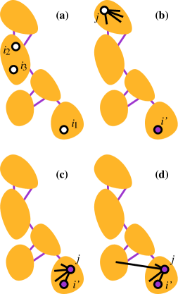
Figure 1: Illustration of the networked seceder model. (a) In step 1 three vertices, $i_{1}$, $i_{2}$ and $i_{3}$, are chosen at random. (b) In step 2 the least central of the three vertices is relabeled to $\hat{i}$. In step 3 a vertex $j$ is selected at random and (c) the edges of $j$ are rewired to $\hat{i}$ and $\hat{i}$s neighborhood (and to a set of random other vertices if necessary. Note that, in (c), $j$ is moved to the cluster it is rewired to. In step 4 $j$’s edges are rewired with a probability $p$. The shaded areas represent tightly connected subgraphs.

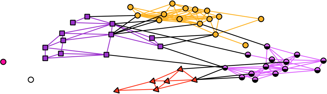
Figure 2: One realization of the networked seceder model. The model parameters are $N=50$, $M=150$ and $p=0$. The indicated groups are identified with Newman’s clustering algorithm (see Sect. II.3). This realization have modularity $Q=0.575$, clustering coefficient $C=0.530$, and assortative mixing coefficient $r=0.0456$.

II.2 The seceder model

The original seceder model sec1 is based on $N$ individuals with a real number $s(i)$ representing the traits (or personality) of individual $i$. The algorithm is then to repeat the following steps:

1. Select three individuals $i_{1}$, $i_{2}$ and $i_{3}$ with uniform randomness.

2. Pick the one (we call it $\hat{i}$) of these whose $s$-value is farthest away from the average $[s(i_{1})+s(i_{2})+s(i_{3})]/3$.

3. Replace the $s$-value of a uniformly randomly chosen agent with $s(\hat{i})+\eta$, where $\eta$ is a random number from the normal distribution with mean zero and variance one.

Note that the actual values of $s$ is irrelevant, only the differences between $s$ of different agents. The output of the seceder model is a complex pattern of individuals that stick together in well-defined groups. The groups has a life-cycle of their own—they are born, spawn new groups and die. Statistical properties of the model is investigated in Ref. sec1 , effects of a bounded trait-space is studied in Ref. sec2 , the fitness landscape is the issue of Ref. sec3 , and Ref. sec4 presents a generalization to higher-dimensional trait-spaces.

Our generalization of this model to a network model based on the idea that if the system is embedded in a network, then the difference in personality is implicitly expressed through the network position, so the identity number (or vector) $s$ becomes superfluous. I.e., the homophily assumption mcp:bird —that like attracts like—means that the difference in character between two vertices $i$ and $j$ (defined as $|s(i)-s(j)|$ in the traditional seceder model) can be estimated by the graph distance $d(i,j)$ in a networked model. The model we propose is then, starting from any graph with $N$ vertices and $M$ edges, to iterate the following steps:

1. Select three different vertices $i_{1}$, $i_{2}$ and $i_{3}$ with uniform randomness.

2. Pick the one $\hat{i}$ of these that is least central in the following sense: If the graph is connected vertices of highest eccentricity are the least central. If the graph is disconnected the most eccentric vertices within the smallest connected subgraph are the least central. If more than one vertex is least central, let $\hat{i}$ be a vertex in the set of least central vertices chosen uniformly randomly.

3. Choose a vertex $j$ by uniform randomness. If $\deg j\leq\deg\hat{i}+1$, rewire $j$’s edges to $\hat{i}$ and a random selection of $\hat{i}$’s neighbors. If $\deg j\geq\deg\hat{i}+1$, rewire $j$’s edges to $\hat{i}$, $i$’s neighborhood and (if $\deg j>\deg\hat{i}+1$) to $\deg j-\deg\hat{i}-1$ randomly selected other vertices.

4. Go through $j$’s edges once more and rewire these with a probability $p$ to a randomly chosen vertex.

The rewiring of steps 3 and 4 are performed with the restriction that no multiple edges or loops (edges that goes from a vertex to itself) are allowed. Steps 1 to 3 correspond rather closely to the same steps of the original model. That $j$’s edges are rewired mainly to the neighborhood of $\hat{i}$ (and $\hat{i}$ itself) reflects the inheritance of trait value of the original model—by the homophily assumption the neighborhood of $\hat{i}$ will have much the same personality as $\hat{i}$ itself. The main difference between original and the networked seceder model is step 4 where some vertices are rewired to distant vertices. The motivation for this step is that long-range connections exists in real-world networks wattsstrogatz ; watts:small2 , and can in some situations be even more important than the strong links of a cohesive group grano:weak . This kind of rewiring, to obtain long-range connections has been used to model “small-world behavior” of networks wattsstrogatz (i.e. a logarithmic, or slower, scaling of the average inter-vertex distance for ensembles of graphs with the same average degree mejn:rev ).

To make the model consistent we also have to specify the initial graph. As far as we can see, at least for finite $p$, this choice is irrelevant—the structure of the generated graphs are the same (or at least very similar). We will not investigate this point further. Instead we fix the initial graph to an instant of Erdös and Rényi’s random graph model er:on (for a modern survey of this model, see Ref. janson ): A graph with $N$ edges and $M$ edges is constructed by starting from isolated vertices and then iteratively introduce edges between vertex-pairs chosen by uniform randomness and with the restriction that no multiple edges or loops are allowed. To be sure that the structure of the random graph is gone we run the construction algorithm $10N$ sweeps through every vertex before the graph is sampled. (We justify this number a posteriori below.)

An illustration of the construction algorithm can be seen in Fig. 1. An realization of the algorithm is displayed in Fig. 2. The $p$-value of this realization is zero. For the value $p=0.1$ we use in most simulations the community structure is less visible to the eye. Nevertheless—as we will see—the community structure is still substantial for much larger values of $p$.

II.3 Detecting communities

To analyze the structure of cohesive subgroups in our model networks we use the community detection scheme presented in Ref. mejn:fast . This algorithm starts from one-vertex clusters and (somewhat reminiscent of the algorithm in Ref. bohu:soc ) iteratively merges clusters to form clusters of increasing size with relatively few edges to the outside. The crucial ingredient in the scheme is a quality function

$$Q^{\prime}=\sum_{s\in S}(e_{ss}-a_{s}^{2})$$ (1)

where $S$ is the set of subnetworks at a specific iteration of the algorithm and $e_{ss^{\prime}}$ is the fraction of edges that goes between a vertex in $s$ and a vertex in $s^{\prime}$, and $a_{s}=\sum_{s^{\prime}}e_{ss^{\prime}}$. The algorithm performs a steepest-accent in $Q^{\prime}$-space—at each iteration the two clusters that leads to the largest increase (or smallest decrease) in $Q^{\prime}$ are merged. The iteration having the highest $Q^{\prime}$ value—which defines the modularity $Q$—gives the partition into subgroups.

II.4 Conditional uniform graph tests

One can argue that some network structures are more basic than other. Given such an assumption and a network $G$, an interesting issue is whether a certain structure, say $X$, is an artifact of a more basic structure, say $Y$. One way to do this is by a conditional uniform graph test: One compares the value of $X(G)$ with $X$ averaged over an ensemble of graphs with a the value of $Y$ fixed to $Y(G)$. This has (since Ref. katz:cug ) been a well established technique in social network analysis and has recently been brought over to physicists’ maslov:inet and biologists’ alon network literature. A common assumption alon ; maslov:inet ; roberts:mcmc is that the degree distribution is such a very basic structure. We make this assumption too and perform a conditional uniform graph test with respect to the degree sequence of the networks. To sample networks with a given degree sequence we use the idea of Ref. roberts:mcmc to rewire the edges of the network in such a way that the degree sequence remains unaltered. More precisely we go through all edges $(i,j)\in E$ and perform the following:

1. Construct the set $E^{\prime}$ of edges such that if $(\hat{i},\hat{j})\in E^{\prime}$ then replacing $(i,j)$ and $(\hat{i},\hat{j})$ by $(i,\hat{j})$ and $(\hat{i},j)$ would not introduce any loops (self-edges) or multiple edges.

2. Pick an edge $(\hat{i},\hat{j})\in E^{\prime}$ by uniform randomness.

3. Rewire $(i,j)$ to $(i,\hat{j})$ and $(\hat{i},\hat{j})$ to $(\hat{i},j)$.

For every realization of the seceder algorithm we sample $n_{\mathrm{sample}}=10$ randomized reference networks as described above. The motivation for this rather low number is that all quantities seems to be self-averaging (the fluctuations decrease with $N$) and many have symmetric distributions with respect to rewirings (which makes many realization averages compensate for few rewiring averages). To further motivate this small $n_{\mathrm{sample}}$ we compare with $n_{\mathrm{sample}}=100$ for the smallest size ($N=200$, which, as mentioned, is most affected by fluctuations) and find that the quantities typically differ by $0.5\%$ which we consider small.

III The community structure of the seceder model

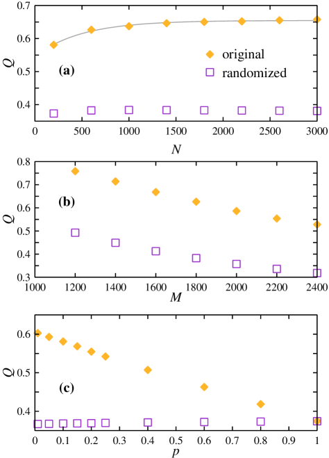
Figure 3: The modularity $Q$ as a function of the model parameters. (a) shows $Q$ as a function of $N$ with $M=3N$ and $p=0.1$. (b) displays $Q$ for different $M$ for $N=600$ and $p=0.1$. In (c) we plot the $p$ dependence of $Q$ for $N=200$ and $M=600$. The gray line in (a) is a fit to a exponential. All errorbars are smaller than the symbol size.

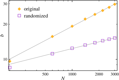
Figure 4: The number of groups $b$ as a function of the systems size $N$. The other parameter values are $M=3N$ and $p=0.1$. The line is a fit to a power-law $ab^{\beta}$. For this set of parameters $\beta=0.400(6)$ for the seceder model and $0.193(6)$ for the reference-graphs of the conditional uniform graph test. All errorbars are smaller than the symbol size. Note the double-logarithmic scale.

The key quantity capturing the degree of community order in the network is the modularity $Q$ (defined in Sect. II.3)). In Fig. 3(a) we see that, if the average degree and $p$ is kept constant $Q$ converges to a high value, $Q\approx 0.64$ for $p=0.1$ and $M=3N$. This value is much higher than the reference value from the randomized networks—this curve has a peak around $N=1500$ and decays for larger $N$, larger sizes would be needed to see of $Q$ converges to a finite value for the randomized networks. With the analogy to the Watts-Strogatz model (where a fraction $p$ of a circulant’s harary edges is rewired randomly) we would say that $p=0.1$ is a rather high value, still $Q$ is much higher for the networked seceder model than for random networks with the same degree distribution. From this we conclude that our model fulfills its purpose—it produces networks with a pronounced community structure just as the original seceder model makes agents divide into well-defined groups in trait-space. In Fig. 3(b) we plot the $M$-dependence of $Q$ for fixed $N=600$ and $p=0.1$. We see that $Q$ decreases with $M$ for both the seceder model and the randomized networks. As $M$ approaches its maximum value $N(N-1)/2$ the curves will converge (since the fully connected graph is unique), but the figure shows that the curves are separated for a wide parameter range. More importantly it suggests that the quantity $Q$ should be rescaled by some appropriate function if networks of different average degree are to be compared. In the rest of our paper, however, we will keep the degree constant. In Fig. 3(c) we show the $p$-dependence of $Q$. As expected $Q$ decays monotonously, in fact almost linearly, with $p$. The curves for the seceder model converges to the curve of the randomized networks as $p\rightarrow 0$. $Q$ of the randomized reference networks is almost $p$-independent. The fact that it is not completely $p$-independent means that the degree distribution of the seceder model must vary with $p$. We will strengthen this claim later.

Fig. 4 shows the size-dependence of $b$—the number of groups. We see that this function can be well-described by a constant plus a power-law,

$$A+b^{\beta}~{},$$ (2)

(where $A$ is a constant) with an exponent $\beta=0.400(6)$ for the seceder model and $\beta=0.193(6)$ for the random networks with the same degree distribution. The average community-size is given by $N/b$ and will therefore also behave as a power-law, with exponent $1-\beta=0.600(6)$. This fact that for the number and average size of the communities grows with $N$ does not seem contradictory to the real world to us. Since a community, both in a social and economical interpretation of the model, does not need to be controlled or supervised there is no natural upper limit to the number of community members. Furthermore, there is no particular constraint on the number of communities present in real world systems. A thorough study of the scaling-exponents would be interesting, but falls out of the scope of the present paper.

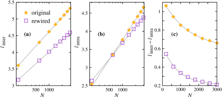
Figure 5: Average distance between and within clusters (as identified by the algorithm described in Sect. II.3). The gray lines are fits to an exponential form. The slope of the original is the same in (a) and (b) (also the rewired line has the same slope in (a) and (b)). All errorbars are smaller than the symbol size.

In Fig. 5 we display the average geodesic lengths within a community $l_{\mathrm{intra}}$ and between vertices of different communities $l_{\mathrm{inter}}$ for parameter values $M=3N$ and $p=0.1$. To be precise, we consider the largest connected component (which typically contains $99\%$ of the vertices), and define

$$l_{\mathrm{intra}}=\frac{1}{N_{\mathrm{intra}}}\sum_{i=1}^{b}\sum_{v,w\in B^{i}}d(v,w)\mbox{~{}and}$$ (3a)

$$l_{\mathrm{inter}}=\frac{1}{\dbinom{N}{2}-N_{\mathrm{intra}}}\sum_{i=1}^{b}\sum_{v\in B^{i}}\sum_{w\notin B^{i}}d(v,w)$$ (3b)

where $B^{i}$ is the $i$’th cluster and

$$N_{\mathrm{intra}}=\sum_{i=1}^{b}\dbinom{i}{2}$$ (4)

is the number of pairs of vertices belonging to the same community. As seen in Fig. 5(a) and (b) both $l_{\mathrm{intra}}$ and $l_{\mathrm{inter}}$ grows logarithmically as functions of $N$ with the same slope in a semi-logarithmic plot. A logarithmic scaling of the average shortest path length (which of course also holds) is expected (cf. Ref. bollobas_chung_88 ). But we could not anticipate the lack of qualitative difference between distances between vertices of the same an different clusters. The actual values of $l_{\mathrm{intra}}$ is significantly smaller than $l_{\mathrm{inter}}$ and this difference holds as $N\rightarrow\infty$: As seen in Fig. 5(c) $l_{\mathrm{inter}}-l_{\mathrm{intra}}$ converges to $0.60(1)$. The same value for the randomized graphs is $l_{\mathrm{inter}}-l_{\mathrm{intra}}=0.204(8)$ which is expected—the detected communities in the networked seceder model are more well-defined and tight-knit that the corresponding communities in a random network with the same degree distribution.

IV Other structural characteristics

Apart from the quantities of the previous section, all directly related to the community structure, we also look at some other well established structural measures: The clustering coefficient, the assortative mixing coefficient and the degree distribution.

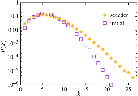
Figure 6: Degree distribution of the networked seceder model. The model parameters are $N=1800$, $M=5400$ and $p=0.1$. The squares indicate the degree distribution of a random graph with the sizes ($N$ and $M$), i.e., the initial network before the iterations of the seceder model commence—see Eq. (5).

IV.1 Degree distribution

Following the works of Barabási and coworkers ba:model ; alb:attack ; bara:www the degree distribution has been perhaps the most studied network structure. Many of these studies have found a skewed, power-law tailed, degree-distribution. In some social networks—of telephone calls aiello , e-mail communication bornholdt:email and the network of sexual contacts liljeros:sex —authors have found large tails of the degree distribution that fits well to a power-law functional form. Other social network studies report degree distributions with large degree cut-offs, these contain network of movie actor amaral:classes , scientific collaborations mejn:scicolpnas or Internet community interaction pok or romantic interaction among High School students (the network of Ref. addh as studied in Ref. mejn:rev ). Yet other studies have found social networks with Gaussian degree distributions (the acquaintance networks of Refs. fararo and ber:mormon studied in Ref. amaral:classes ), or exponential degree distributions (of e-mail networks mejn:email ; gui:sesi ). We conclude that the degree distribution of social networks is still an open question with, most likely, not a single solution—different social networks may follow different degree distributions. The degree distribution of the networked seceder model is displayed in Fig. 6. We note that $P(k)$ has an exponential tail, notably larger than the Poisson degree distribution doromen:rev

$$P(k)=e^{-\bar{k}}\frac{\bar{k}^{k}}{k!}$$ (5)

(where $\bar{k}=2M/N$ is the mean degree) of the initial random graph, but far from as wide as a power-law. Clearly this falls into one of the cases mentioned above. We note that as $p$ grows the degree distribution gets closer to the original network (this was anticipated in Sect. III).

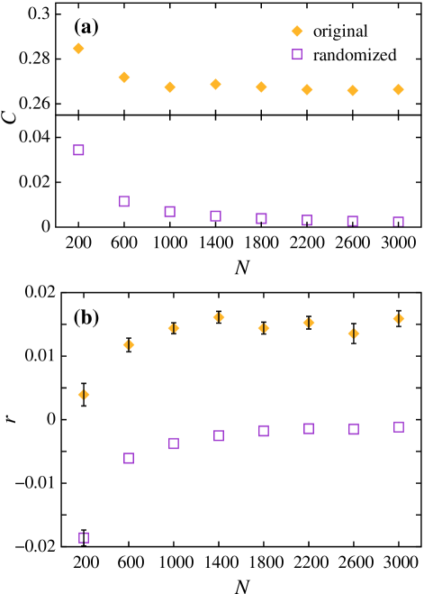
Figure 7: Common structural measures. (a) shows the clustering coefficient as a function of the number of vertices for the seceder model and rewired networks. (b) displays the corresponding plot of the assortative mixing coefficient. The network parameters are $M=3N$ and $p=0.1$. Error bars are shown if they are larger than the symbol size.

IV.2 Clustering coefficient

The clustering coefficient $C$ measures the fraction of connected triples of vertices that form a triad. This type of statistics has been popular since Ref. wattsstrogatz . The definition we use is slightly different from that of Ref. wattsstrogatz :

$$C=\frac{c(3)}{p(3)}~{},$$ (6)

where $c(n)$ denotes ten number of representations of circuits of length $n$ and $p(n)$ denotes the number of representations of paths of length $n$. (By ‘representation’ we mean an ordered triple such that one vertex is adjacent to the vertex before or after. For example, a triangle has six representations—all permutations of the three vertices.) This definition is common in sociology (although sociologists emphasize triad statistics for directed networks)—see Ref. leik:book for a review—but is also frequent in physicists’ literature since Ref. bw:sw . A plot of $C$ as a function of $N$ is shown in Fig. 7(a). We see that $C$ for the seceder model converges to a constant value rather rapidly. Similarity the $C$ for the rewired networks goes to zero roughly over the same time scale. The fact that community structure induces a high clustering is well known and modeled mejn:clumodel , as is the fact that the clustering vanishes like $1/N$ in a random graph with Poisson degree distribution mejn:rev .

IV.3 Assortative mixing coefficient

The assortative mixing coefficient mejn:assmix is the Pearson correlation coefficient of the degrees at either side of an edge:

$$r=\frac{4\langle k_{1}\,k_{2}\rangle-\langle k_{1}+k_{2}\rangle^{2}}{2\langle k_{1}^{2}+k_{2}^{2}\rangle-\langle k_{1}+k_{2}\rangle^{2}}$$ (7)

where subscript $i$ denotes the $i$th argument and average is over the edge set. $r$ is known to be positive in many social networks mejn:assmix ; mejn:mix (networks of online interaction does not seem to follow this rule pok ). It has been suggested that this assortative mixing can be related to community structure mejn:why . Against this backdrop it is pleasing, but not surprising, to note that the networked seceder model produces networks with markedly positive $r$, see Fig. 7(b). The reference networks with the same degree sequences converges to zero from negative values, as also observed in Ref. pok . It has been argued maslov:inet ; mejn:oricorr that networks formed by agents without any preference for the degrees of the neighboring vertices gets negative $r$ from the restriction that only one edge can go between one pair of vertices. This is probably the reason for the negative $r$ values of the rewired networks.

V Characteristics of community dynamics

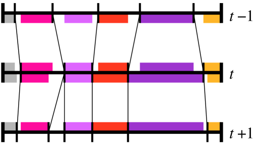
Figure 8: Illustration of the identification of clusters at consecutive time steps. The vertex set is represented by the horizontal line. The vertical tics demarcate cluster boundaries. The communities at consecutive time step is matched so that the overlap (the horizontal sum of shaded segments) is maximized.

Figure 9: Community dynamics for a typical run with the parameter values $N=100$, $M=300$ and $p=0$ and 100 iterations of the networked seceder model. The different panels shows different statistics for one single run of the algorithm. (a) shows the time evolution of the assortative mixing coefficient. (b) shows the clustering coefficient $C$. (c) shows the modularity $Q$. (d) shows the maximal overlap $y$ between consecutive time steps. (e) illustrates the time evolution of the communities. A vertical cross section of (e) gives the respective relative sizes of the different clusters. The clusters are sorted horizontally according to age—the oldest clusters are in the top of the panel.

In this section we look at the dynamics of the communities. To do this we need criteria for if a cluster $B_{k}^{t}$ at time $t$ is the same as cluster $B_{k^{\prime}}^{t-1}$ at time $t-1$. The idea is to find the best possible matching of vertices between the partition into clusters of the two consecutive time steps. To give a mathematical definition, let $\mathcal{B}_{t}=\{B_{t}^{1},\cdots,B_{t}^{b(t)}\}$ be the partition of $G_{t}$ into clusters by the algorithm described in Sect. II.3 and let $b^{\prime}=\min(b(t),b(t-1))$. Now we define a mapping $f$ from $b^{\prime}$ elements of $[1,b(t-1)]$ to $b^{\prime}$ elements of $[1,b(t)]$ such that the overlap

$$y^{\prime}_{t}=\sum_{k=1}^{b^{\prime}}|B^{k}_{t-1}\cap B^{f(k)}_{t}|$$ (8)

is maximized ($|\>\cdot\>|$ denotes cardinality). Let $y(t)$ denote this maximized $y^{\prime}_{t}$ value. To calculate this overlap we use the straightforward method of testing all matchings. In principle this algorithm runs in exponential time, but since the number of groups is typically rather low systems of a few hundred vertices numerically tractable.

The evolution of the group structure, with the group structure identified as described above, is displayed in Fig. 9. In Figs. 9(a) and (b) we see the time evolution of the assortative mixing coefficient $r$ and the clustering coefficient $C$, whose average size-scaling was studied in Sect. IV. We note that the assortative mixing coefficient fluctuates rather much. Even though it is mostly positive (remember that the average value is significantly positive) it also have rather pronounced negative values. This is likely to be a finite size phenomenon—as the assortative mixing coefficient is self-averaging pok , larger systems would not fluctuate much and have stable positive values (as seen in Fig. 7(b)). The clustering coefficient as displayed in Fig. 9(b) shows a more stable evolutionary trajectory. Over a time scale roughly corresponding to $N=100$ updating steps $C$ goes from the value of the initial Erdös-Rényi value to the higher clustering coefficient of the networked seceder model. This is natural since it is also roughly the time scale for all vertices to be picked and rewired once. The value of the modularity $Q$, displayed in Fig. 9(c), is shows a similar behavior as the clustering coefficient as it increases from the value $\sim 0.4$ of the original random graph to $\sim 0.6$ of the seceder model. $C$ and $Q$ seem to be strongly correlated, something that seems very logical in the context of the seceder model—the clustering coefficient increases when a high degree vertex is rewired to a specific cluster, a process that also strengthens the community structure. If this strong $C$-$Q$ correlation is a more ubiquitous property is an interesting problem for future studies. In Fig. 9(d) we plot the overlap $y$ which fluctuates between $25$ and $75$ with an average well below $50$. These values are lower than we expected a priori, as it means than identity of more than half the group members changes a typical time step. Just as the fluctuations in $r$, we expect the fluctuations in the cluster structure to decrease with system size, therefore $y/N$ will increase with $N$. In Fig. 9(e) the time development of different cluster sizes is illustrated. A horizontal cross section gives the size partitioning of the vertex set at a given time step. A demarcated area represents a group. Older groups are above younger groups. An observation from Fig. 9(e) is that groups typically lives between one and 100 time steps. The life-time scale of groups seems to coincide with that of the initial relaxation to the seceder equilibrium. We also note that there seems to be no particular correlation between age and stability or size, a situation that would have produced skewed life time or cluster size distributions. At the bottom of the diagram, hardly visible, there are numerous small, short-lived, clusters. This is an effect of isolates constantly present in the system (for this set of parameter values there are typically one or two at a time step).

The observations in this section were checked for a few other runs and seems to be representative. Since they do not hint some surprising phenomena (against the backdrop of the previous sections and the algorithm itself) we do not conduct any extensive statistical survey of the dynamical properties.

VI Summary and conclusions

We have proposed a model for network formation based on the seceder model. The model captures how a community structure can emerge from the desire to be different, both in social and economic systems. The community structure of our model is analyzed with a recent graph clustering scheme. This scheme has the advantage that it gives a measure of the degree of community structure in a network—the modularity $Q$. We see that the $Q$ is much higher for our model networks than for random reference networks with the same degree distributions. Both the number of groups and the average of size of groups growth as power-laws with sub-linear exponents. Both the average geodesic distance between vertices of the same and different clusters grows logarithmically; the difference between these, however, is much larger for the networked seceder model than for the random reference networks. The general picture is thus the the networked seceder model generates well-defined communities just like the agents of the original seceder model gets clustered in trait space.

The networked seceder model gives networks of high clustering and positive assortative mixing by degree—properties that are known to be characteristic of acquaintance networks. The degree distribution has a peak around the average degree and a exponentially decaying, also that consistent with real world observations.

The dynamics of the communities were briefly investigated by defining a mapping between consecutive time steps that maximizes an overlap function. Using this method we conclude that the speed of the dynamics is set by the size of the system. We see that the clustering coefficient and modularity are strongly correlated and that older groups are not necessarily larger than younger.

To epitomize, the networked seceder model gives an mechanism of emergent community structure that is different from earlier proposed mechanisms in network models motter:sn ; jin:mo ; skyrms:mo . The mechanism is arguably present in, at least, social networks kamp:at . We speculate that this model can be applied to networks of companies that are linked if they are active in the same market.

Ackowledgenments

Thanks are due to Beom Jun Kim, Fredrik Liljeros, Petter Minnhagen and Mark Newman. The authors were partially supported by the Swedish Research Council through contract no. 2002-4135.

References

- (1) W. Aiello, F. Chung, and L. Lu, A random graph model for massive graphs, in Proceedings of the 32nd Annual ACM Symposium on Theory of Computing, New York, 2000, Association of Computing Machinery, pp. 171-180.
- (2) R. Albert and A.-L. Barabási, Statistical mechanics of complex networks, Rev. Mod. Phys 74 (2002), pp. 47-98.
- (3) R. Albert, H. Jeong, and A.-L. Barabási, Attack and error tolerance of complex networks, Nature 406 (2000), pp. 378-382.
- (4) L. A. N. Amaral, A. Scala, M. Barthélémy, and H. E. Stanley, Classes of small-world networks, Proc. Natl. Acad. Sci. USA 97 (2000), pp. 11149-11152.
- (5) A.-L. Barabási and R. Albert, Emergence of scaling in random networks, Science 286 (1999), pp. 509-512.
- (6) A.-L. Barabási, R. Albert, H. Jeong, and G. Bianconi, Power-law distribution of the world wide web, Science 287 (2000), p. 2115.
- (7) A. Barrat and M. Weigt, On the properties of small-world network models, Eur. Phys. J. B 13 (2000), pp. 547-560.
- (8) P. S. Bearman, J. Moody, and K. Stovel, Chains of affection: The structure of adolescent romantic and sexual networks. preprint submitted to Am. J. Soc.
- (9) H. R. Bernard, P. D. Kilworth, M. J. Evans, C. McCarty, and G. A. Selley, Studying social relations cross-culturally, Ethnology 27 (1988), pp. 155-179.
- (10) R. D. Bock and S. Z. Husain, An adaptation of Holzinger’s B-coefficients for the analysis of sociometric data, Sociometry 13 (1950), pp. 146-153.
- (11) B. Bollobás and F. R. K. Chung, The diameter of a cycle plus a random matching, SIAM J. Discrete Math. 1 (1988), pp. 328-333.
- (12) G. Bonanno, G. Caldarelli, F. Lillo, and R. N. Mantegna, Topology of correlation based minimal spanning trees in real and model markets. e-print cond-mat/0211546.
- (13) F. Buckley and F. Harary, Distance in graphs, Addison-Wesley, Redwood City, 1989.
- (14) P. Dittrich, The seceder effect in bounded space, InterJournal (2000), art. no. 363.
- (15) P. Dittrich and W. Banzhaf, Survival of the unfittest? The seceder model and its fitness landscape, in Advances in Artificial Life (Proceedings of the 6th European Conference on Artificial Life, Prague, September 10-14, 2001), J. Kelemen and P. Sosik, eds., Springer, Berlin, 2001, pp. 100-109.
- (16) P. Dittrich, F. Liljeros, A. Soulier, and W. Banzhaf, Spontaneous group formation in the seceder model, Phys. Rev. Lett. 84 (2000), pp. 3205-3208.
- (17) S. N. Dorogovtsev and J. F. F. Mendes, Evolution of networks, Adv. Phys. 51 (2002), pp. 1079-1187.
- (18) H. Ebel, L.-I. Mielsch, and S. Bornholdt, Scale-free topology of e-mail networks, Phys. Rev. E 66 (2002), art. no. 035103.
- (19) P. Erdös and A. Rényi, On random graphs I, Publ. Math. Debrecen 6 (1959), pp. 290-297.
- (20) T. J. Fararo and M. H. Sunshine, A study of a biased friendship net, Syracuse University Press, Syracuse, NY, 1964.
- (21) M. Girvan and M. E. J. Newman, Community structure in social and biological networks, Proc. Natl. Acad. Sci. USA 99 (2002), pp. 7821-7826.
- (22) P. Gleiser and L. Danon, Community structure in jazz. e-print cond-mat/0307434.
- (23) M. S. Granovetter, The strength of weak ties, Am. J. Sociol. 78 (1973), pp. 1360-1380.
- (24) R. Guimerà, L. Danon, A. Díaz-Guilera, F. Giralt, and A. Arenas, Self-similar community structure in organisations. e-print cond-mat/0211498.
- (25) P. Holme, C. R. Edling, and F. Liljeros, Structure and time-evolution of the Internet community pussokram.com. e-print cond-mat/0210514.
- (26) S. Janson, T. Łuczac, and A. Ruciński, Random Graphs, Whiley, New York, 1999.
- (27) E. M. Jin, M. Girvan, and M. E. J. Newman, The structure of growing social networks, Phys. Rev. E 64 (2001), art. no. 046132.
- (28) C. Kampmeier and B. Simon, Individuality and group formation: The role of independence and differentiation, Journal of Personality and Social Psychology 81 (2001), pp. 448-462.
- (29) L. Katz and J. H. Powell, Probability distributions of random variables associated with a structure of the sample space of sociometric investigations, Annals of Mathematical Statistics 28 (1957), pp. 442-448.
- (30) R. K. Leik and B. F. Meeker, Mathematical sociology, Prentice-Hall, Englewood Cliffs, NJ, 1975.
- (31) F. Liljeros, C. R. Edling, L. A. Nunes Amaral, H. E. Stanley, and Y. Åberg, The web of human sexual contacts, Nature 411 (2001), p. 907.
- (32) S. Maslov, K. Sneppen, and A. Zaliznyak, Pattern detection in complex networks: Corelation profile of the Internet. e-print cond-mat/0205379.
- (33) J. M. McPherson and J. R. Ranger-Moore, Evolution on a dancing landscape: Organizations and networks in dynamic blau space, Social Forces 70 (1991), pp. 19-42.
- (34) J. M. McPherson, L. Smith-Lovin, and J. Cook, Birds of a feather: Homophily in social networks, Annual Review of Sociology 27 (2001), pp. 415-444.
- (35) A. E. Motter, T. Nishikawa, and Y.-C. Lai, Large-scale structural organization of social networks, Phys. Rev. E 68 (2003), art. no. 036105.
- (36) M. E. J. Newman, Fast algorithm for detecting community structure in networks. e-print cond-mat/0309508.
- (37) , The structure of scientific collaboration networks, Proc. Natl. Acad. Sci. USA 98 (2001), pp. 404-409.
- (38) , Assortative mixing in networks, Phys. Rev. Lett. 89 (2002), art. no. 208701.
- (39) , Mixing patterns in networks, Phys. Rev. E 67 (2003), art. no. 026126.
- (40) , Properties of highly clustered networks, Phys. Rev. E 68 (2003), art. no. 026121.
- (41) , The structure and function of complex networks, SIAM Rev. 45 (2003), pp. 167-256.
- (42) M. E. J. Newman, S. Forrest, and J. Balthrop, Email networks and the spread of computer viruses, Phys. Rev. E 66 (2002), art. no. 035101.
- (43) M. E. J. Newman and M. Girvan, Finding and evaluating community structure in networks. e-print cond-mat/0308217.
- (44) M. E. J. Newman and J. Park, Why social networks are diffrent from other types of networks, Phys. Rev. E 68 (2003), art. no. 036122.
- (45) J. Park and M. E. J. Newman, Origin of degree correlations in the Internet and other networks, Phys. Rev. E 68 (2003), art. no. 026112.
- (46) F. Radicchi, C. Castellano, F. Cecconi, V. Loreto, and D. Parisi, Defining and identifying communities in networks. e-print cond-mat/0309488.
- (47) J. M. Roberts Jr., Simple methods for simulating sociomatrices with given marginal totals, Soc. Netw. 22 (2000), pp. 273-283.
- (48) S. Shen-Orr, R. Milo, S. Mangan, and U. Alon, Network motifs in the transcriptional regulation network of Escherichia coli, Nature Genetics 31 (2002), pp. 64-68.
- (49) B. Skyrms and R. Freemantle, A dynamic model of social network formation, Proc. Natl. Acad. Sci. USA 97 (2000), pp. 9340-9346.
- (50) A. Soulier and T. Halpin-Healy, The dynamics of multidimensional secession: Fixed points and ideological condensation, Phys. Rev. Lett. 90 (2003), art. no. 258103.
- (51) K. Taro Greenfeld, Speed tribes: Days and nights with Japan’s next generation, Perennial, New York, 1995.
- (52) D. J. Watts, Networks, dynamics, and the small world phenomenon, Am. J. Sociol. 105 (1999), pp. 493-592.
- (53) D. J. Watts and S. H. Strogatz, Collective dynamics of ‘small-world’ networks, Nature 393 (1998), pp. 440-442.