Entanglement Energetics at Zero Temperature

Abstract

We show how many-body ground state entanglement information may be extracted from sub-system energy measurements at zero temperature. Generically, the larger the measured energy fluctuations are, the larger the entanglement is. Examples are given with the two-state system and the harmonic oscillator. Comparisons made with recent qubit experiments show this type of measurement provides another method to quantify entanglement with the environment.

A many-body quantum system is cooled to zero temperature so that it is forced into its overall nondegenerate ground state. We discuss the measurement of a sub-system Hamiltonian and demonstrate that it can be found in an excited state with a probability that depends on the coupling to its environment. This non-intuitive result is a pure quantum phenomenon: it is a consequence of entanglement sch of the sub-system with the environment. In fact, we demonstrate that knowledge of the probability to find the system in an excited state can be used to determine the degree of entanglement of the sub-system and bath. Consequently, simple systems with well known isolated quantum mechanical properties (such as the two-state system and harmonic oscillator) become “entanglement-meters”.

There is growing interest of ground-state entanglement in condensed matter physics. Theoretical works on ground state entanglement have addressed entropy scaling in harmonic networks ms , spin-spin entanglement in quantum spin chains arnesen and quantum phase transitions fazio ; nielsen2 . Entanglement properties of the ground state are also essential in the field of adiabatic quantum computing adiabatic . Furthermore it is interesting to link other ground state properties like the persistent current of small mesoscopic rings pc ; pc2 , or of doubly connected Cooper pair boxes cpbox1 ; cpbox2 ; qubit , or the occupation of resonant states resonant to the zero-temperature entanglement energetics.

We consider a general Hamiltonian $H=H_{s}+H_{c}+H_{E}$, that couples $(c)$ the system $(s)$ we are interested in to a quantum environment $(E)$ such as a network of harmonic oscillators rmp . The lowest energy separable state is $|\Omega\rangle=|0\rangle_{s}|0\rangle_{E}$, where $|0\rangle_{\{s,E\}}$ are the lowest uncoupled energy state of both systems. However, if the system Hamiltonian and the total Hamiltonian do not commute (which is the generic situation), then $|\Omega\rangle$ is not an energy eigenstate of the total Hamiltonian. Thus, there must be a lower energy eigenstate ($|0\rangle$) of the total Hamiltonian which is by definition an entangled state. Because time evolution is governed by the full Hamiltonian, the ground state expectation of any operator with no explicit time dependence will have no time evolution, insuring that any measurement is static in time. This situation is in contrast to the usual starting point of assuming that the initial state is a separable state and studying how it becomes entangled. The reduced density operator of the system is given by tracing out the environmental degrees of freedom, $\rho={\rm Tr}_{E}|0\rangle\langle 0|$. Assuming the full state of the whole system is pure, the reduced density matrix contains all accessible system information, including entanglement of the system with its environment. Because repeated measurements of $H_{s}$ will give different energies as the sub-system is not in an energy eigenstate, we are interested in a complete description of the statistical energy fluctuations. These fluctuations may be described in two equivalent ways. The first way is to find the diagonal density matrix elements in the basis where $H_{s}$ is diagonal. These elements represent the probability to measure a particular excited state of $H_{s}$. A second way is to find all energy cumulants. A cumulant of arbitrary order may be calculated from the sub-system energy generating function, $Z(\chi)=\langle\exp(-\chi H_{s})\rangle$ (as always, $\langle{\cal O}\rangle={\rm Tr}\rho{\cal O}$) so that the n^th energy cumulant is given by

$$\langle\langle H_{s}^{n}\rangle\rangle=(-)^{n}\frac{d^{n}}{d\chi^{n}}\ln Z(\chi)\Big{|}_{\chi=0}\;.$$ (1)

These cumulants give information about the measured energy distribution around the average.

Before proceeding to calculate these energy fluctuations, we ask a general question about entanglement. Given the energy distribution function (the diagonal matrix elements of the density matrix only), can anything be said in general about the purity or entropy of the state? Surprisingly, because we are given the additional information that we are at zero temperature, the answer is yes. If we ever measure the sub-system’s energy and find an excited energy, then we know the state is entangled. Though this statement alone links energy fluctuations with entanglement, a further quantitative statement may be made in the weak coupling limit. The reason for this is the following: the assumptions exponentially suppress higher states, so to first order in the coupling constant, we can consider a two-state system where the density matrix has the form $\rho_{--}=1-\alpha p$, $\rho_{++}=\alpha p$, $\rho_{+-}=\rho_{-+}^{\ast}=\alpha c$. For vanishing coupling constant $\alpha=0$, this just gives the density matrix for the separable state. The linear dependence of $\rho$ on $\alpha$ holds to first order for the model systems considered below and is the entanglement contribution. If one measures the diagonal elements of $\rho$, one obtains $\rho_{--}$ and $\rho_{++}$ as the probability to be measured in the ground or excited state (because $\alpha$ is small, there is only a small probability to find the sub-system in the upper state). If we now diagonalize $\rho$, the eigenvalues are $\lambda_{\pm}=\{1-p\,\alpha,p\,\alpha\}+{\cal O}(\alpha^{2})$. To first order in $\alpha$, the eigenvalues are the diagonal matrix elements, so we may (to a good approximation) write the purity or entropy in terms of these probabilities even if the energy difference remains unknown.

The Qubit. Let us now first evaluate the energy fluctuations of a qubit, a two-state system. The most general (trace 1) spin density matrix is $\rho=({\openone}+\langle\sigma_{x}\rangle\sigma_{x}+\langle\sigma_{y}\rangle\sigma_{y}+\langle\sigma_{z}\rangle\sigma_{z})/2$. A simple measure of the entanglement is given by the purity, ${\rm Tr}\rho^{2}=(1/2)(1+X^{2}+Y^{2}+Z^{2})$, where $X_{i}=\langle\sigma_{i}\rangle$. It is well known that $(X,Y,Z)$ form coordinates in the Block sphere. Purity lies at the surface where $X^{2}+Y^{2}+Z^{2}=1$, whereas corruption lies deep in the middle.

We take the system Hamiltonian note1 to be $H_{s}=(\epsilon/2)\,\sigma_{z}+(\Delta/2)\,\sigma_{x}$. Introducing the frequency $\Omega=\sqrt{\epsilon^{2}+\Delta^{2}}/\hbar$ and using the identity $e^{-i\frac{\beta}{2}{\hat{n}}\cdot{\hat{\sigma}}}={\rm}I\cos\frac{\beta}{2}-i{\hat{n}}\cdot{\hat{\sigma}}\sin\frac{\beta}{2}$ with $\beta=\chi\Omega$, it is straightforward to show

$$Z(i\chi)=\cos(\Omega\chi/2)-i\frac{\sin(\Omega\chi/2)}{\Omega}(\epsilon\langle\sigma_{z}\rangle+\Delta\langle\sigma_{x}\rangle)\,.$$ (2)

The energy probability distribution may be easily found by Fourier transforming Eq. (2), or by tracing in the diagonal basis of the system Hamiltonian. The answer may be expressed with only the average energy, $\langle H_{s}\rangle=\frac{\epsilon}{2}\langle\sigma_{z}\rangle+\frac{\Delta}{2}\langle\sigma_{x}\rangle$ as a sum of delta functions at the system energies $\pm\hbar\Omega/2$ with weights of the diagonal density matrix elements,

$$\rho_{++,--}=(1/2)\left[1\pm\frac{\langle H_{s}\rangle}{\hbar\Omega/2}\right]\,.$$ (3)

Clearly, if the spin is isolated from the environment, $\langle H_{s}\rangle=-\hbar\Omega/2$, the ground state energy, the probability weight to be in an excited state vanishes. This distribution may also be found from knowledge of the isolated eigenenergies, the fact that $\langle H_{s}\rangle=\sum_{j}E_{j}\rho_{jj}$, and that Tr$\rho=1$. This later argument may be extended to $n$-state systems given the first $n-1$ moments of the Hamiltonian and the $n$ eigenenergies.

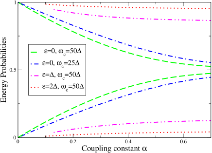
Figure 1: Energy probabilities $p_{up}$ and $p_{down}$ for the spin-boson problem. With increasing coupling to the environment it it is more likely to measure the qubit in the excited state. For the symmetric case $(\epsilon=0)$, we use the Bethe ansatz solution, while for the general case, we use a perturbative solution which is only valid for large $\epsilon$ or large $\alpha$.

Connection with Real Qubits. The probability weights depend on the energy parameters $\epsilon$ and $\Delta$, and the expectation values of the Pauli matrices. For real qubits produced in the lab, these will depend on the environment spin-boson . Often, we can link the basic phenomena we have been describing to physical measurements other than energy. For example, in a mesoscopic ring threaded by an Aharonov-Bohm flux $\Phi$, or for the Cooper pair box, the tunneling matrix element depends on flux $\Delta(\Phi)$. The operator one is interested in measuring is given by the normalized persistent current pc , or the expectation of $\sigma_{x}$ (for the symmetric case of $\epsilon=0$),

$$\langle\sigma_{x}\rangle=\frac{I(\Phi)}{I_{0}(\Phi)}\;,$$ (4)

where $I_{0}(\Phi)$ is the uncoupled value of the persistent current. A common model for environmental effects is given by coupling the two-state system to a series of harmonic oscillators, the spin-boson model rmp ; pc ; weiss ; spin-boson . In Fig.(1) we have plotted the upper and lower occupation probabilities for the spin-boson model as a function of the coupling constant $\alpha$. For the symmetric case ($\epsilon=0$), we have used the Bethe ansatz solution pc ; bethe , while for $\epsilon$ finite, we have used the perturbative solution in $\Delta/\omega_{c}$ which is valid only for larger $\alpha$ or $\epsilon$ pc . Thus the plot is cut off at a small $\alpha$. A computational approach calculating the expectation values of the Pauli matrices over the whole parameter range was given in Ref. spin-boson . For $\epsilon=0$, Eq. (4) determines also the expectation value of $H_{s}$, and thus the weights of the energy distribution function, Eq. (3), are directly related to the persistent current.

Experiments are always carried out at finite temperature, and it is important to demonstrate that there exists a cross-over temperature to the quantum behavior discussed here. In the low temperature limit, the thermal occupation probability is $p_{up}=e^{-(E_{2}-E_{1})/kT}$. In the weak coupling limit for the symmetric spin boson problem, the probability to measure the excited state scales as $p_{up}=-\alpha\log(\Delta/\omega_{c})$ note2 . Setting these factors equal and solving for $T^{\ast}$ yields

$$kT^{\ast}=-\frac{E_{2}-E_{1}}{\log(\alpha\log\frac{\omega_{c}}{\Delta})}\,.$$ (5)

Since $T^{\ast}$ scales as the inverse logarithm of the coupling constant, it is experimentally possible to reach a regime where thermal excitation is negligible.

As an order of magnitude estimate, we compare with the Cooper pair box cpbox1 ; cpbox2 which is among the most environmentally isolated solid state qubits qubit . From cpbox2 which found a $Q\sim 10^{4}$, we estimate the quantum probability for the box to be measured in the excited state as $p_{up}\sim 10^{-3}-10^{-4}$, which is of same order or larger than the thermal probability, $p_{th}\sim 10^{-4}$. Experimentally, $p_{up}$ and $p_{th}$ may be confused by fitting data with an effective temperature, $\rho_{th}=\exp(-\beta_{\rm eff}H_{s})$ note3 . However, one may distinguish true thermal behavior from the effect described here because $p_{up}$ and $p_{th}$ depend differently on tunable system parameters such as $\Delta$. In fact, $\beta_{\rm eff}$ is an entanglement measure. This chain of reasoning may be inverted to provide an estimate for $Q$ given only $p_{up}$.

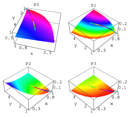
Figure 2: The probability to measure a harmonic oscillator in the ground and first three excited states as a function of $x$ and $y$ (see text). The line traces out the behavior of the ohmic bath as a function of the coupling in the under-damped range.

The Harmonic Oscillator. We now consider the entanglement energetics of a harmonic oscillator, $H_{s}=p^{2}/(2m)+(1/2)m\omega^{2}q^{2}$. Since there are an infinite number of states, the problem is harder. To simplify our task, we assume a linear coupling with a harmonic oscillator bath. This implies that the density matrix is Gaussian so that environmental information is contained in the second moments $\langle q^{2}\rangle$ and $\langle p^{2}\rangle$ weiss ; ms ,

$$\langle q|{\rho}|q^{\prime}\rangle=\frac{1}{\sqrt{2\pi\langle q^{2}\rangle}}\exp\left\{-\frac{(\frac{q+q^{\prime}}{2})^{2}}{2\langle q^{2}\rangle}-\frac{\langle p^{2}\rangle(q-q^{\prime})^{2}}{2\hbar^{2}}\right\}.$$ (6)

Expectation values of higher powers of $H_{s}$ are non-trivial because $q$ and $p$ do not commute. The purity of the density matrix Eq. (6) is

$${\rm Tr}\rho^{2}=\int dqdq^{\prime}\langle q|\rho|q^{\prime}\rangle\langle q^{\prime}|\rho|q\rangle=\frac{\hbar/2}{\sqrt{\langle q^{2}\rangle\langle p^{2}\rangle}}\,.$$ (7)

The uncertainty relation, $\sqrt{\langle q^{2}\rangle\langle p^{2}\rangle}\geq\hbar/2$, guarantees that ${\rm Tr}\rho^{2}\leq 1$, with the inequality becoming sharp if the oscillator is isolated from the environment. As the environment causes greater deviation from the Planck scale limit, the state loses purity.

The generating function $Z$ may be calculated conveniently by tracing in the position basis and inserting a complete set of position states between the operators,

$$Z(\chi)=\int dqdq^{\prime}\langle q|\rho|q^{\prime}\rangle\langle q^{\prime}|e^{-\chi H_{s}}|q\rangle.$$ (8)

The first object in Eq. (8) is the density matrix in position representation, given by Eq. (6). The second object may be interpreted as the uncoupled position-space propagator of the harmonic oscillator from position $q$ to $q^{\prime}$ in time $-i\hbar\chi$. We find

$$Z=\left\{2E\,\frac{\sinh\varepsilon\chi}{\varepsilon}+2A\,(\cosh\varepsilon\chi-1)+\frac{1+\cosh\varepsilon\chi}{2}\right\}^{-\frac{1}{2}}$$ (9)

where $\varepsilon=\hbar\omega$, $2E=m\omega^{2}\langle q^{2}\rangle+\langle p^{2}\rangle/m$ and $A=\langle q^{2}\rangle\langle p^{2}\rangle/\hbar^{2}$. $E$ is the average energy of the oscillator, while $A\geq 1$ is a measure of satisfaction of the uncertainty principle. Eq. (9) has a pleasing limit for the free particle $\omega\rightarrow 0$,

$$Z(\chi)_{free}=\left\{1+\chi\langle p^{2}\rangle/m\right\}^{-\frac{1}{2}}\,,$$ (10)

which is just the generating function for Wick contractions, $\langle p^{2n}\rangle=(2n-1)!!\,(\langle p^{2}\rangle)^{n}$. Thus, in Eq. (9), the inverse square root generates the right combinatorial factors under differentiation, and the nontrivial $\chi$ dependence accounts for the commutation relations between $q$ and $p$. The first few harmonic oscillator energy cumulants may now be straightforwardly found via Eq. (1),

$$\langle\langle H_{s}^{2}\rangle\rangle = (1/2)[-(\varepsilon^{2}/2)+4E^{2}-2\varepsilon^{2}A]\;,$$ (11)

$$\langle\langle H_{s}^{3}\rangle\rangle = -(E/2)[-16E^{2}+\varepsilon^{2}(1+12A)]\;,$$ (12)

$$\langle\langle H_{s}^{4}\rangle\rangle = 48E^{4}-4\varepsilon^{2}E^{2}(1+12A)$$ (13)

$$+ \varepsilon^{4}[(1/8)+2A+6A^{2}]\,.$$

After inserting the mean square values for an ohmic bath (see the discussion above eqs. (15,16)), Eq. (11) is identical to the main result of Ref. nb .

Alternatively, we now consider the diagonal matrix elements $\rho_{nn}$. An analytical expression for the density matrix in the energy basis may be found by using the wavefunctions of the harmonic oscillator, $\psi_{n}(q)\propto e^{-\gamma^{2}q^{2}/2}H_{n}(\gamma q)$ where $\gamma=\sqrt{m\omega/\hbar}$ and $H_{n}(x)$ is the $n^{th}$ Hermite polynomial. In the energy basis, the density matrix is given by $\rho_{nm}=\int dqdq^{\prime}\psi^{\ast}_{n}(q)\langle q|\rho|q^{\prime}\rangle\psi_{m}(q^{\prime})$. The position space integrals may be done using two different copies of the generating function for the Hermite polynomials. The diagonal elements may be found by equating equal powers of the generating variables. We first define the dimensionless variables $x=2\gamma^{2}\langle q^{2}\rangle$, $y=2\langle p^{2}\rangle/(\gamma^{2}\hbar^{2})$, and $D=1+x+y+xy$. $x$ and $y$ are related to the major and minor axes of an uncertainty ellipse. The isolated harmonic oscillator (in it’s ground state) obeys two important properties: minimum uncertainty (in position and momentum) and equipartition of energy between average kinetic and potential energies. The influence of the environment causes deviations from these ideal behaviors which may be accounted for by introducing two new parameters, $a=(y-x)/D,\;b=(xy-1)/D$ with $-1\leq a\leq 1$ and $0\leq b\leq 1$. The deviation from equipartition of energy is measured by $a$, while the deviation from the ideal uncertainty relation is measured by $b$. We find

$$\rho_{nn}=\frac{n!}{2^{n}}\sqrt{\frac{4}{D}}\sum_{m=0}^{n}\sum_{p=0}^{n}\frac{(a^{2})^{p}(2b)^{m}}{m!(p!)^{2}}\delta_{n,m+2p}\,.$$ (14)

All terms are positive (because $a$ appears only squared), less than one, and obey ${\rm Tr}\rho=1$. The summation over $m$ and $p$ define a polynomial $P_{n}$ of order $n$ in $a$ and $b$. The probability for the lone oscillator to be measured in an excited state clearly decays rapidly with level number. These probabilities also reveal environmental information. For example, $P_{1}=2b$ and is thus only sensitive to the area of the state, while $P_{2}=a^{2}+2b^{2}$ depends on both the uncertainty and energy asymmetry. Additionally, if we expand the first density matrix eigenvalue ms ; weiss with respect to small deviations of $x$ and $y$, we recover $\rho_{11}$ in agreement with our general argument.

Although $x$ and $y$ have been treated as independent variables, the kind of environment the system is coupled to replaces these variables with two functions of the coupling constant. For example, with the ohmic bath weiss ; nb (in the under-damped limit), the variables are

$$x(\alpha)=\frac{1}{\sqrt{1-\alpha^{2}}}\left(1-\frac{2}{\pi}{\rm arctan}\frac{\alpha}{\sqrt{1-\alpha^{2}}}\right)\;,$$ (15)

$$y(\alpha)=(1-2\alpha^{2})x(\alpha)+\frac{4\alpha}{\pi}\ln\frac{\omega_{c}}{\omega}\;,$$ (16)

where $\alpha$ is the coupling to the environment in units of the oscillator frequency and $\omega_{c}$ is a high frequency cutoff. This bath information is shown in Fig. (2) with $\omega_{c}=10\omega$. The trajectory of the line over the surface shows how the probabilities evolve as the coupling $\alpha$ is increased from 0 to 1. Other kinds of environments would trace out different contours on the probability surface.

In conclusion, we have shown that projective measurements of the system Hamiltonian at zero temperature reveals entanglement properties of the many-body quantum mechanical ground state. Consequently, repeated experiments on simple quantum systems give information about the nature of the environment, the strength of the coupling and entanglement. The larger the energy fluctuations, the greater the entanglement. There are several possibilities for experimental implementations. We have mentioned measurement of persistent current pc ; pc2 as well as projecting on the system’s energy eigenstates. Another measurement possibility is a zero temperature activation-like process act where the dominant mechanism is not tunneling, but the same quantum effects of the environment which we have discussed here.

This work was supported by the Swiss National Science Foundation.

References

- (1) E. Schrödinger, Naturwissenschaften 23, 807 (1935); J. S. Bell, Physics 1, 195 (1964); M. A. Nielsen, and I. L. Chuang, Quantum Computation and Quantum Information, (Cambridge University Press, 2000).
- (2) M. Srednicki, Phys. Rev. Lett. 71, 666 (1993).
- (3) M. C. Arnesen, S. Bose, and V. Vedral, Phys. Rev. Lett. 87, 017901 (2001).
- (4) T. J. Osborne, M. A. Nielsen, Phys. Rev. A 66, 032110 (2002).
- (5) A. Osterloh, et. al. Nature 416, 608 (2002).
- (6) G. Falci, et. al., Nature 407, 355 (2000).
- (7) P. Cedraschi, V. V. Ponomarenko, M. Büttiker, Phys. Rev. Lett. 84, 346 (2000).
- (8) F. Marquardt and C. Bruder, Phys. Rev. B 65, 125315 (2002); F. Guinea, Phys. Rev. B 67, 045103 (2003); D. S. Golubev, C. P. Herrero, A. D. Zaikin, Europhys. Lett. 63, 426 (2003); O. Entin-Wohlman, Y. Imry, A. Aharony, Phys. Rev. Lett. 91, 046802 (2003).
- (9) V. Bouchiat, et. al., Phys. Scr. T76, 165 (1998).
- (10) Y. Nakamura, Yu. A. Pashkin, and J. S. Tsai, Nature 398, 786 (1999).
- (11) D. Vion, et. al., Science 296, 886 (2002).
- (12) A. Furusaki and K. A. Matveev Phys. Rev. Lett. 88, 226404 (2002).
- (13) A. J. Leggett, et. al., Rev. Mod. Phys. 59, 1 (1987).
- (14) U. Weiss, Quantum Dissipative Systems, (World Scientific, 2000).
- (15) T. A. Costi, and R. H. McKenzie, Phys. Rev. A 68, 034301 (2003).
- (16) V. V. Ponomarenko, Phys. Rev. B 48, 5265 (1993).
- (17) K. E. Nagaev and M. Büttiker, Europhys. Lett. 58, 475 (2002).
- (18) D. Arteaga, et. al., Int. J. Theor. Phys. 42, 1247 (2003).
- (19) All system parameters include the high-frequency renormalization (Frank-Condon effect weiss ).
- (20) is the high frequency cutoff needed to regularize the theory.
- (21) cannot always be written as an effective thermal distribution. Ref. ms explicitly demonstrates this if the system contains two or more oscillators.