Motion in random fields - an application to stock market data

Abstract

A new model for stock price fluctuations is proposed, based upon an analogy with the motion of tracers in Gaussian random fields, as used in turbulent dispersion models and in studies of transport in dynamically disordered media. Analytical and numerical results for this model in a special limiting case of a single-scale field show characteristics similar to those found in empirical studies of stock market data. Specifically, short-term returns have a non-Gaussian distribution, with super-diffusive volatility, and a fast-decaying correlation function. The correlation function of the absolute value of returns decays as a power-law, and the returns distribution converges towards Gaussian over long times. Some important characteristics of empirical data are not, however, reproduced by the model, notably the scaling of tails of the cumulative distribution function of returns.
PACS numbers: 05.60.-k, 89.65.Gh, 05.40.-a, 02.50-r

1 Introduction

Random fluctuations in stock market prices have long fascinated investors and mathematical modelers alike. Although the investors’ hopes of accurately predicting tomorrow’s share price appear to be in vain, models which limit themselves to statistical characteristics such as distributions and correlations have had some success. Bachelier’s classical model [1] treats the stock price $S(t)$ as a random walk, leading to the conclusion that the distribution of prices is Gaussian. Samuelson [2] instead describes the log-price

$$x(t)=\ln[S(t)/S(0)]$$ (1)

as a random walk, and therefore concludes that the stock price $S(t)$ should have a log-normal distribution. This model remains in common usage, despite the shortcomings listed below, not least because it permits the derivation of an equation for pricing options and other financial derivatives, e.g., the famous Black-Scholes equation [3]. Nevertheless, empirical evidence from stock market data indicates that the random walk model inadequately describes many important features of the stock price process. The following stylized facts are accepted as established by these studies [3, 4]:

• Short-term returns are non-Gaussian, with ‘fat tails’ and high central peaks. The center of the returns distribution is well fitted by Lévy distributions [5]. Recent studies indicate that the tails of the returns distribution decay as power-laws [6]. As the lag time increases, the returns distributions slowly converge towards Gaussian; recent analysis of the Standard & Poor 500 index (S&P500) estimates this convergence is seen only on lags longer than 4 days [6].

• The correlation function of returns decays exponentially over a short timescale, consistent with market efficiency. However, the correlation function of the absolute value of the returns shows a much slower (power-law) decay [6].

• The volatility (standard deviation of returns) grows like that of a diffusion (random walk) process, i.e. as the square root of the lag time, for lag times longer than about 10 minutes. However, higher frequency (shorter lag) returns demonstrate a super-diffusive volatility, which can be fitted to power-laws with exponents found to range between 0.67 and 0.77 [6, 7].

• The distribution of stock price returns exhibits a simple scaling: in [5] a power-law scaling of the peak of the returns distribution $P(0)$ with lag time is shown to hold across many magnitudes of lag times. The exponent of the power-law is approximately $-0.7$.

Most of the references cited here examine data from the Standard & Poor 500 index (S&P500), but other international markets are found to behave similarly [6].

The predictions of the random-walk model can be investigated using the random differential equation

$$\frac{dx}{dt}=u_{w}(t),$$ (2)

which yields the log price $x(t)$ from each realization of the random function $u_{w}(t)$. The classical random walk follows from taking $u_{w}(t)$ to be a Gaussian white-noise process with zero mean and (auto)correlation function [8]:

$$\left<u_{w}(t)u_{w}(t^{\prime})\right>=\alpha^{2}\delta(t-t^{\prime}),$$ (3)

where $\delta(t)$ is the Dirac delta function, and the angle brackets denote averaging over time or over an ensemble of realizations. White noise is the formal derivative of a Wiener process, which connects (2) to rigorous methods for stochastic differential equations [9]. Note that throughout this paper all stochastic processes are assumed (unless explicitly stated otherwise) to have zero mean, zero drift, and to be statistically stationary.

Equation (2) is easily solved, and leads to results which do not agree with the empirical facts (i)-(iv) listed above. Defining the return on the stock price $S(t)$ at time $t$ as the forward change in the logarithm of $S(t)$ over the lag time $\Delta$:

$$r_{\Delta}(t) = x(t+\Delta)-x(t)$$ (4)

$$= \ln S(t+\Delta)-\ln S(t),$$

it is found that the white-noise case leads to probability distribution functions (PDFs) for $r_{\Delta}$ which are Gaussian at all lags $\Delta$, in contrast to (i). The lack of memory effects in white-noise leads to correlation functions which decay immediately to zero, unlike (ii). The volatility grows diffusively for all lag values, and so has no super-diffusive range, while the scaling of $P(0)$ follows a power-law different from that found for actual prices, see (iv) above.

A natural generalization of the white-noise model again takes a form similar to (2)

$$\frac{dx}{dt}=u_{c}(t),$$ (5)

but with $u_{c}(t)$ now being a non-white or colored process, incorporating some memory effects. For the particularly simple case of Gaussian noise, it can be described fully by its correlation function

$$\left<u_{c}(t)u_{c}(t^{\prime})\right>=\alpha^{2}R(t-t^{\prime}).$$ (6)

Here $R(t)$ decays from a maximum of unity at $t=0$ to zero as $t\rightarrow\infty$, and $\alpha^{2}$ is the variance of the process $u_{c}$. Gaussian noise is attractive because it appears naturally as the limiting sum of many independent noise sources under the central limit theorem [8], and because of its analytical tractability. Indeed equation (5) is again easily solvable for Gaussian $u_{c}$, but leads once more to Gaussian-distributed returns at all lag times, in contrast to (i). Moreover, the correlation of absolute returns does not decay more slowly that the returns correlation, as required by (ii).

These failings of simple differential equation models have inspired many attempts to reproduce the empirical facts (i)-(iv) using various stochastic models. As a sample of just a few of these, we list the truncated Lévy flights model [10, 11], ARCH and GARCH models [12, 13], non-Gaussian Ornstein-Uhlenbeck processes [14], and a model based on a continuous superposition of jump processes [15, 7]. The first three of these were reviewed in [16]. An ideal model should reproduce all the experimental facts (i)-(iv), by giving a simple picture of the stochastic process underlying the stock price time series, but no model has yet been found which fulfills all these criteria [17].

In this paper we examine the results of generalizing the random walk models (2) and (5) to motion in a random field:

$$\frac{dx}{dt}=u(x,t).$$ (7)

Here $u(x,t)$ is a Gaussian random field with zero mean, which is fully described by its correlation function

$$\left<u(x,t)u(x^{\prime},t^{\prime})\right> = \alpha^{2}Q(x-x^{\prime},t-t^{\prime})$$ (8)

$$= \alpha^{2}S(x-x^{\prime})R(t-t^{\prime}).$$ (9)

For simplicity we take the field to be homogeneous and stationary; the factorization in (9) of the correlation into separate time- and $x$-correlations is for ease of exposition only, and more complicated inter-dependent correlations can be considered. The averaging procedure in equation (8) is over an ensemble of realizations of the random field $u$, or using a uniform measure over all possible $(x,t)$ values.

Equation (7) implies that the log-price $x(t)$ changes in a random fashion, but the rate of change is randomly dependent on both time and the current value of $x$. Note that random-walk models (2) and (5) may be recovered by taking $S(x)\equiv 1$ and choosing the time correlation $R(t)$ appropriately. We will show that the $x$-dependence in the noise term yields qualitatively different results to the random walk models, and that many of the empirical observations (i)-(iv) of stock markets may be reproduced by (7).

The $x$-dependent noise term in (7) is motivated by recent studies in turbulent dispersion [18] and transport in dynamically disordered media [19]. These investigations employ equation (7), but with a rather different interpretation: $x(t)$ is the position vector (in 2 or 3 dimensions) of a passive tracer, and $u(x,t)$ is the velocity vector field which transports the tracer. The tracer is called passive because it is assumed not to affect the velocity field by its presence, and so $u(x,t)$ is a prescribed random field. An instructive example is the motion of a small buoy on the surface of the ocean [20]: the two-dimensional vector $x(t)$ then describes the position of the buoy (by its longitude and latitude, say) while the tracer is moved by the ocean waves according to (7), with the Gaussian field $u(x,t)$ providing an approximate description of the ocean wave field.

The distribution of such tracers resulting from motion in a Gaussian field is known to be non-Gaussian, at least over short to intermediate timescales [18, 21]. Crucial to understanding this effect is the difference between the Eulerian velocity $u(x,t)$, i.e., the velocity measured at the fixed location $x$ at time $t$, and the Lagrangian velocity

$$v(t)=u(x(t),t),$$ (10)

which is the time series of velocity measurements made by the tracer itself as it moves through the random field [22]. When there is no $x$-dependence in the velocity field $u$, the Eulerian and Lagrangian velocities coincide, but otherwise a Gaussian Eulerian velocity field can yield non-Gaussian Lagrangian processes. The relationship between Eulerian and Lagrangian random processes is an active research area, especially in the case of a compressible (non-zero divergence) velocity field which is of interest here [23, 24, 25].

Our model of the log-price uses a scalar “position” $x(t)$ and “velocity” $u(x,t)$ rather than the vector-valued analogues in the turbulent dispersion problems described above. Nevertheless, the concept of Eulerian and Lagrangian velocities carries over to the one-dimensional case, and so we will refer to $x(t)$ as the “price tracer”, with its “velocity” $u(x,t)$ related by equation (7). The fact that the Eulerian velocity field $u(x,t)$ is Gaussian allows us to obtain analytical results, and may be justified as a consequence of the central limit theorem applied to the sum of many independent forces on stock prices. In this paper we will not further pursue a microeconomic justification [26, 27] for (7), but rather concentrate on demonstrating that it may yield some of the observed statistical properties of empirical stock market data.

The remainder of this paper is structured as follows. In section 2 the consequences of the $x$-dependence of the noise in equation (7) are examined through some simple examples, and a special limiting case (single-scale field) is highlighted. The statistics of the Lagrangian velocity (10) in the single-scale case are found analytically in sections 3 and 4, and are related to the statistics of the returns $r_{\Delta}$. Numerical simulations of equation (7) are considered in section 5, and a simple method for generating Monte-Carlo time series in the single-scale case is found. Results from such simulations are presented in section 6, and compared to the stylized facts (i)-(iv), as presented in [6] and [5]. Section 7 comprises of discussion of the results and directions for future work.

2 X-dependent velocity fields

The concept of $x$-dependence in the velocity of the log-price $x(t)$ was introduce in section 1. To gain some intuitive understanding of the effect of such $x$-dependence, we first return to the random walk model with colored noise $u_{c}(t)$, independent of $x$, as in (5) and (6):

$$\frac{dx}{dt}=u_{c}(t)\text{, with }\left<u_{c}(t)u_{c}(t^{\prime})\right>=\alpha^{2}R(t-t^{\prime}).$$ (11)

For clarity, we consider in this section a specific form for the time correlation $R(t)$:

$$R(t)=\exp\left(-\frac{t^{2}}{2T^{2}}\right),$$ (12)

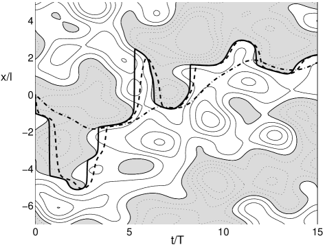
Figure 2: Motion of stock tracers in a random field which depends on both time and $x$, as in (7). The correlation functions are (12) and (13), and the values of $\epsilon$ are: $\epsilon=1.0$ (dash-dotted), $\epsilon=0.1$ (dashed), and $\epsilon=0.01$ (solid).

where a characteristic decay time $T$ has been introduced. Figure 1 shows the contours of a single realization of the $x$-independent $u_{c}(t)$, negative values of the velocity being denoted by shaded areas and dotted contour lines. Time increases along the horizontal axis, with the stock log price $x$ measured on the vertical axis. The motion of a stock tracer with initial condition $x(0)=0$ is shown also; note the negative rate of change of stock price in the shaded regions (negative velocity), and the positive rate of change in the regions where $u>0$. Because there is no $x$-dependence in (11), the velocity field depends only on time, and so the contours are vertical lines. By contrast, a simple $x$-dependent velocity field of the type proposed in (7) has a non-trivial $x$-correlation function $S(x)$ in equation (9); for example in Fig. 2 we use

$$S(x)=\exp\left(-\frac{x^{2}}{2l^{2}}\right),$$ (13)

where $l$ defines a correlation scale ($l\rightarrow\infty$ recovers the $x$-independent case). The contours in Fig. 2 display a more complicated structure than in Fig. 1, and this is reflected in the observed motion of the stock prices. The three parameters $\alpha$, $T$ and $l$ characterizing the random field may be combined into one dimensionless quantity

$$\epsilon=\frac{l}{\alpha T},$$ (14)

and if the time, log price and velocity are re-scaled using these parameters:

$$t = T\tilde{t}$$

$$x = l\tilde{x}$$

$$u = \alpha\tilde{u},$$ (15)

then the equation of motion (7) becomes

$$\epsilon\frac{d\tilde{x}}{d\tilde{t}}=\tilde{u}(\tilde{x},\tilde{t}).$$ (16)

Note that the re-scaled velocity field $\tilde{u}$ has unit variance. In Fig 2. the stock price motions resulting from solving (16) are shown for $\epsilon$ values of $\epsilon=1$, $\epsilon=0.1$, and $\epsilon=0.01$. When $\epsilon$ is large, the length scale $l$ of the randomness in $x$ is much larger than the effect $\alpha T$ of the random variation in time — this is analogous to the case of weak space dependence in turbulent dispersion problems studied in [18] using perturbation theory. In the case of $\epsilon\gg 1$, small deviations of the stock price distribution from a Gaussian shape are found, with kurtosis less than 3. However, the studies of empirical data mentioned in section 1 indicate that the kurtosis of stock returns is much larger than 3, and so the weakly space-dependent theory does not seem relevant here.

The opposite limit, i.e., $\epsilon\ll 1$ appears more promising. In Fig. 2, we observe that the stock prices for parameter values $\epsilon=0.1$ and $\epsilon=0.01$ display some interesting generic features. Constrained by the equation of motion to move downwards in shaded regions (where the velocity $\tilde{u}$ is negative), and upwards in unshaded regions, the stock tracers tend to become trapped near curves of $\tilde{u}=0$, with $\tilde{u}$ positive below them and negative above them. These stable positions disappear when the zero-velocity manifold ‘folds over’, and the stock tracer is then driven by equation (16) to move quickly to another slow manifold. A complete understanding of the dynamics of the system as $\epsilon\rightarrow 0$ requires a singular perturbation approach [29] to equation (16), but the important feature for our work is the following of the zero-velocity manifold by the stock tracer, punctuated by fast jumps.

An analytical approach to the general $\epsilon\rightarrow 0$ case has not yet been found, but some interesting features are highlighted by choosing a particularly simple form for the $x$-correlation function:

$$S(x)=\cos(kx),$$ (17)

where $k$ is a constant. This correlation function corresponds to a so-called ‘single-scale’ Gaussian velocity field, which (as shown in [30]) can always be written in the form

$$u(x,t)=f(t)\cos(kx)+g(t)\sin(kx),$$ (18)

where $f(t)$ and $g(t)$ are independent Gaussian random functions of time, each with zero mean, variance $\alpha^{2}$, and a given correlation function $R(t)$:

$$\left<f(t)f(t^{\prime})\right>=\left<g(t)g(t^{\prime})\right>=\alpha^{2}R(t-t^{\prime}).$$ (19)

An example of motion in such a single-scale field is shown in Fig. 3. Note the periodicity in the vertical direction, and the lack of jumps. In the remainder of this paper we will concentrate on this simplified example and show that many of the statistical characteristics of the resulting stock returns are remarkably similar to those observed in empirical data.

3 Lagrangian velocity and PDF

In this section we consider the statistical characterization of motion along the $u=0$ curves of the single-scale random field (18), according to the equation of motion (7), and with the Gaussian random functions $f(t)$ and $g(t)$ defined as in (19). Again, the analogue with tracer motion on the surface of a turbulence ocean proves instructive. The Eulerian velocity at a point $x$ at time $t$ is defined by the random field (18). Each tracer particle moving through this field will, however, experience its own time history of velocity variations; this is called the Lagrangian velocity of the tracer $v(t)$. The crucial point in our use of random-field models of stock price motion is that the Eulerian field may, as in (18), have Gaussian statistics, while the Lagrangian velocity (that is, the velocity ‘felt by the tracer’) need not be Gaussian. Some intuitive notion of why this might be may be gained from considering the fact that the velocity at space-time points $(x,t)$ picked at random from the Eulerian field has a Gaussian distribution; on the other hand, the dynamics of the tracer particles mean that they are more likely to cluster in regions of low velocity, with high-velocity transitions between, meaning both zero values of $v$ and high values are more likely than for a Gaussian distribution. This argument holds for any random field, but as we show in this section, a quantitative description may be derived in the case of a single-scale field (17) for the $\epsilon\rightarrow 0$ limit.

In the limit of small $\epsilon$, we saw in the previous section that the stock tracer motion is confined to curves with $u=0$. While the Eulerian velocity on these curves is zero by definition, the Lagrangian velocity is non-zero, as the tracer moves to remain on the $u=0$ curve. In fact, the Lagrangian velocity felt by the particle trapped on such a curve is given by

$$v(t)=\frac{\left.\frac{\partial u}{\partial t}\right|_{u=0}}{\left.\frac{\partial u}{\partial x}\right|_{u=0}},$$ (20)

with the derivatives evaluated on the curve $u=0$. For the single scale field (18), an explicit expression for the Lagrangian velocity may be found in terms of the functions $f(t)$ and $g(t)$ and their derivatives:

$$v(t)=\frac{1}{k}\frac{f^{\prime}g-g^{\prime}f}{f^{2}+g^{2}}.$$ (21)

When the Lagrangian velocity $v(t)$ is known, the equation of motion for the tracer is simply

$$\frac{dx}{dt}=v(t),$$ (22)

with solution

$$x(t)=x(0)+\int_{0}^{t}v(t^{\prime})dt^{\prime}.$$ (23)

Similarly, the return on the stock over a time lag of $\Delta$ is given by

$$r_{\Delta}(t) = x(t+\Delta)-x(t)$$ (24)

$$= \int_{t}^{t+\Delta}v(t^{\prime})dt^{\prime}.$$

Clearly the statistics of the returns follow from the statistics of the Lagrangian velocity, indeed for short time lags it might be expected from (24) that

$$r_{\Delta}(t)\approx v(t)\Delta,$$ (25)

so that the distribution of returns, for instance, can be related directly to the distribution of the Lagrangian velocity. We shall see later that (25) is not fully accurate for large values of $v$, but the Lagrangian velocity distribution will still prove extremely useful.

To find the probability distribution function $P(v)$ of the Lagrangian velocity, we first consider the cumulative probability that the Lagrangian velocity $v$ at a given time is greater than some chosen value $V$. According to (21), $v>V$ if and only if

$$f^{\prime}>\frac{f^{2}+g^{2}}{g}kV+\frac{g^{\prime}f}{g}\equiv F,$$ (26)

where we use the symbol $F$ to denote the right-hand-side. Since $f$, $g$, $f^{\prime}$ and $g^{\prime}$ are independent Gaussian random variables at any single moment in time, we denote their PDFs by $P_{f}$, $P_{g}$ etc., and the cumulative probability of the event (26) is

$$C(V)=\int_{-\infty}^{\infty}dg\int_{-\infty}^{\infty}df\int_{-\infty}^{\infty}dg^{\prime}\int_{F}^{\infty}df^{\prime}P_{g}P_{f}P_{g^{\prime}}P_{f^{\prime}}.$$ (27)

The PDF of $v$ then follows from

$$P(v) = \left.-\frac{d}{dV}C(V)\right|_{V=v}$$ (28)

$$= \int_{-\infty}^{\infty}dg\int_{-\infty}^{\infty}df\int_{-\infty}^{\infty}dg^{\prime}P_{g}P_{f}P_{g^{\prime}}\left.P_{f^{\prime}}\right|_{f^{\prime}=F}\left.\frac{\partial F}{\partial V}\right|_{V=v},$$

and the fact that

$$\frac{\partial F}{\partial V}=k\frac{f^{2}+g^{2}}{g}.$$ (29)

Noting that the variances of $f^{\prime}$ and $g^{\prime}$ both equal $-\alpha^{2}R^{\prime\prime}(0)=\alpha^{2}/\tau_{0}^{2}$, where we introduce the notation $\tau_{0}$ for the timescale defined by the initial radius of curvature of the function $R$:

$$\tau_{0}=\frac{1}{\sqrt{-R^{\prime\prime}(0)}},$$ (30)

the integrations over the $f$-$g$ plane may be performed by using polar coordinates $f=r\cos\theta$, $g=r\sin\theta$, yielding

$$P(v) = \int_{-\infty}^{\infty}dg\int_{-\infty}^{\infty}dfP_{g}P_{f}\frac{k\tau_{0}}{\sqrt{2\pi\alpha^{2}}}\sqrt{f^{2}+g^{2}}\exp\left[-(f^{2}+g^{2})\frac{k^{2}\tau_{0}^{2}v^{2}}{2\alpha^{2}}\right]$$ (31)

$$= \frac{k\tau_{0}}{2\left[1+k^{2}\tau_{0}^{2}v^{2}\right]^{\frac{3}{2}}}.$$

The PDF (31) of the Lagrangian velocity $P(v)$ is symmetric in $v$, and so has mean zero. Note that the tails of $P(v)$ decay as $|v|^{-3}$ for large $|v|$, so the variance of $v$ does not exist. Also, (31) effectively contains only one free parameter $k\tau_{0}$, and is otherwise independent of the choice of correlation function $R(t)$ for $f$ and $g$.

4 Correlation of Lagrangian velocity and returns

The (normalized) correlation of the stock returns with lag $\Delta$, at time $t$, is defined by averaging the product of the returns at times separated by $\tau$:

$$\frac{\left<r_{\Delta}(t)r_{\Delta}(t+\tau)\right>}{\left<r_{\Delta}(t)^{2}\right>},$$ (32)

and for stationary returns becomes independent of $t$ . The correlation is normalized by the variance $\left<r_{\Delta}(t)^{2}\right>$ of the returns at lag $\Delta$, which is known as the squared volatility [6]. In this section we derive analytical results to show how the volatility and the returns correlation for a single-scale field with $\epsilon\rightarrow 0$ depend on the time correlation function $R(t)$ of the Eulerian field, and on $\alpha$ and $k$.

Because of the dependence (24) of the returns on the Lagrangian velocity, the correlation of the returns can be written in terms of the correlation function of $v$:

$$\left<r_{\Delta}(t)r_{\Delta}(t+\tau)\right> = \int_{t}^{t+\Delta}dt_{1}\int_{t+\tau}^{t+\tau+\Delta}dt_{2}\left<v(t_{1})v(t_{2})\right>$$ (33)

$$= \int_{0}^{\Delta}dt_{1}\int_{\tau}^{\tau+\Delta}dt_{2}\left<v(t_{1})v(t_{2})\right>$$

$$= \int_{0}^{\Delta}dt_{1}\int_{\tau}^{\tau+\Delta}dt_{2}\,L(t_{1}-t_{2})$$

$$= \int_{0}^{\Delta}(\Delta-t_{1})\left[L(t_{1}-\tau)+L(t_{1}+\tau)\right]dt_{1},$$ (34)

where we have used the stationarity of the returns, and defined the Lagrangian velocity correlation function

$$L(t_{1}-t_{2})=\left<v(t_{1})v(t_{2})\right>.$$ (35)

Note the Lagrangian velocity is assumed to be a stationary process—this has not been proven to follow from Eulerian stationarity in the general case [23], but appears to hold in numerical simulations. We will proceed to calculate $L(t)$, and then use (34) to find the volatility and returns correlation. We note here that when the separation time $\tau$ is much larger than the lag $\Delta$, the returns covariance (34) is approximated by

$$\left<r_{\Delta}(t)r_{\Delta}(t+\tau)\right>\sim\Delta^{2}L(\tau),$$ (36)

consistent with (25).

The correlation function of the stationary random process $v$ is written as an eight-dimensional integral, using the definition (21) of the Lagrangian velocity:

$$L(t) = \left<v(0)v(t)\right>$$

$$= \frac{1}{k^{2}}\int\cdots\int\frac{f_{1}^{\prime}g_{1}-g_{1}^{\prime}f_{1}}{f_{1}^{2}+g_{1}^{2}}\frac{f_{2}^{\prime}g_{2}-g_{2}^{\prime}f_{2}}{f_{2}^{2}+g_{2}^{2}}P_{12}(f_{1},f_{1}^{\prime},f_{2},f_{2}^{\prime})P_{12}(g_{1},g_{1}^{\prime},g_{2},g_{2}^{\prime}).$$

Here the eight-fold integrals are over $f$, $g$, $f^{\prime}$ and $g^{\prime}$ evaluated at each of the two times $t=0$ (with subscript 1) and $t=t$ (subscript 2). The random functions $f$ and $g$ are independent of each other, but the joint probability functions for $f$ and its derivative at different times is found from the Gaussian joint PDF

$$P_{12}(\mathbf{w})=\frac{1}{(2\pi)^{2}}(\text{Det}\mathbf{A})^{\frac{1}{2}}\exp\left[-\frac{1}{2}\mathbf{w}^{T}\mathbf{A}\mathbf{w}\right]$$ (38)

for the vector of arguments, $\mathbf{w}=(f_{1},f_{1}^{\prime},f_{2},f_{2}^{\prime})$, with a similar expression for $g$. The matrix $\mathbf{A}$ is defined by

$$A_{ij}^{-1}=\left<w_{i}w_{j}\right>$$ (39)

and when written out in full:

$$\mathbf{A}^{-1}=\alpha^{2}\left\{\begin{array}[]{cccc}1&0&R(t)&-R^{\prime}(t)\\ 0&-R^{\prime\prime}(0)&R^{\prime}(t)&-R^{\prime\prime}(t)\\ R(t)&R^{\prime}(t)&1&0\\ -R^{\prime}(t)&-R^{\prime\prime}(t)&0&-R^{\prime\prime}(0)\end{array}\right\}.$$ (40)

Using (38) and (40) in (LABEL:Lint) enables us to calculate the Lagrangian correlation $L(t)$. We briefly describe here the steps in the calculation of the multi-dimensional integrals. First, the four integrals over the variables $f_{1}^{\prime}$, $g_{1}^{\prime}$, $f_{2}^{\prime}$, $g_{2}^{\prime}$ are performed - the dependence of the integrand on each of these variables is linear, so the Gaussian integrals may be calculated straightforwardly. For the remaining four variables, we transform to polar coordinates in the $(f_{1},g_{1})$ and $(f_{2},g_{2})$ planes:

$$f_{1}=r\cos\theta,\quad g_{1}=r\sin\theta,\quad f_{2}=\rho\cos\phi,\quad g_{2}=\rho\sin\phi.$$ (41)

The $\phi$ integral is then trivial, and by integrating over $\theta$, $r$, and $\rho$, the final result emerges:

$$L(t)=\frac{1}{2k^{2}R(t)^{2}}\left\{R(t)R^{\prime\prime}(t)-R^{\prime}(t)^{2}\right\}\log\left[1-R(t)^{2}\right].$$ (42)

Equation (42) gives an explicit formula for the Lagrangian velocity correlation in terms of the time correlation $R(t)$ of the single-scale Eulerian field. When the function $R(t)$ is given, $L(t)$ follows immediately from (42), and hence the volatility and returns correlation can be calculated using (34). Before examining the results for the returns, we consider the limiting forms of $L(t)$ for small and large arguments.

Assuming that $R(t)$ is sufficiently smooth near $t=0$ to allow the definition of $\tau_{0}$ as in equation (30), a small-time expansion of (42) yields

$$L(t)\sim-\frac{1}{2k^{2}\tau_{0}^{2}}\log\left(\frac{t^{2}}{\tau_{0}^{2}}\right)\quad\text{ as }t\rightarrow 0.$$ (43)

Note this diverges as $t$ approaches zero, so the variance of the Lagrangian velocity does not exist, in accord with our conclusion at the end of section 3.

For large time arguments, we are particularly interested in power-law decays of correlations, and so consider how the decay of $R(t)$ influences that of $L(t)$. Taking a power-law decay with exponent $-\beta$:

$$R(t)\sim t^{-\beta}\quad\text{ as }t\rightarrow\infty,$$ (44)

the corresponding Lagrangian correlation is found from (42) to decay as

$$L(t)\sim-\frac{\beta}{2k^{2}}t^{-2\beta-2}\quad\text{ as }t\rightarrow\infty.$$ (45)

The negative sign here indicates that the Lagrangian correlation approaches zero from below at large times, being negative whenever $R(t)$ has a power-law decay.

The squared volatility is found by setting $\tau=0$ in (34):

$$\text{vol}^{2}(\Delta)=\left<r_{\Delta}(t)^{2}\right>=2\int_{0}^{\Delta}(\Delta-t)L(t)dt.$$ (46)

For short lags, with $\Delta\ll\tau_{0}$, it follows from (43) that the volatility may be approximated by

$$\text{vol}^{2}(\Delta)\approx\frac{1}{2k^{2}}\frac{\Delta^{2}}{\tau_{0}^{2}}\left[3-\log\left(\frac{\Delta^{2}}{\tau_{0}^{2}}\right)\right]+O\left(\frac{\Delta^{4}}{\tau_{0}^{4}}\right)$$ (47)

Note that while this expression limits to zero as $\Delta$ vanishes, it does not follow a simple power law in $\Delta$ because of the logarithmic term. Although empirical stock volatilities have been fitted with power-laws [6, 7], we show in the next section that (47) can also match the data quite well.

For large time lags $\Delta$, empirical data shows a linear growth in $\text{vol}^{2}$ with $\Delta$. From (46), we can find an expression for the rate of change of $\text{vol}^{2}$ with $\Delta$:

$$\frac{d}{d\Delta}\text{vol}^{2}(\Delta)=2\int_{0}^{\Delta}L(t)dt,$$ (48)

and hence conclude that the squared volatility grows linearly with $\Delta$ for large lags if the integral

$$\int_{0}^{\infty}L(t)dt$$ (49)

has a finite positive value. Assuming a power-law form of $R(t)$ for large arguments, we use the result (45) for the asymptotic form of $L(t)$. It immediately follows that the integral (49) is finite if $\beta>-1/2$, and hence at large lags the squared volatility grows linearly with $\Delta$ in this case.

In empirical stock data, correlations of nonlinear functions of the returns often display significantly slower decay than the correlations of the returns themselves. One quantity of interest is the correlation of absolute returns, which, using (25), may be related to the correlation of absolute Lagrangian velocities (for short lags) as

$$\left<\left|r_{\Delta}(t)\right|\left|r_{\Delta}(t+\tau)\right|\right>-\left<\left|r_{\Delta}(t)^{2}\right|\right>\approx\Delta^{2}\left\{\left<\left|v(t)v(t+\tau)\right|\right>-\left<\left|v(t)^{2}\right|\right>\right\}.$$ (50)

Following similar procedures as in the calculation of $L(t)$, it can be shown that the large-$t$ asymptotics corresponding to a power-law $R(t)\sim t^{-\beta}$ give a correlation of absolute Lagrangian velocities scaling as

$$\left<\left|v(0)v(t)\right|\right>-\left<\left|v^{2}\right|\right>\sim t^{-2\beta}.$$ (51)

In contrast to (45), this correlation remains positive at large times; note too that its rate of decay is slower than that of (45).

Before proceeding to numerical simulations, we briefly summarize the theoretical results. We have obtained the PDF of the Lagrangian velocity in (31), and related the Lagrangian velocity correlation $L(t)$ to the given Eulerian correlation $R(t)$ in (42). This permits estimates of the volatility as a function of lag. Finally, we expect a power-law scaling for the absolute returns correlation when $R(t)$ has a power-law decay. In the following sections we perform numerical simulations to confirm and extend these results.

5 Numerical simulations

To extend the analytical results found in the previous section, we consider the implementation of numerical simulations of motion in random fields. Random fields $u(x,t)$ may be generated using standard techniques [31], with the ordinary differential equation (7) being solved using Runge-Kutta methods. Averages may be calculated over an ensemble of realizations, or over a long time series $x(t)$ in a single realization, to closely mimic the statistical analysis of S&P 500 data performed in [5, 6].

A random field with zero mean and correlation function (9) may be generated using a superposition of random Fourier modes [31]:

$$u(x,t)=\frac{1}{\sqrt{N}}\sum_{n=1}^{N}A_{n}\cos(\omega_{n}t+k_{n}x)+B_{n}\sin(\omega_{n}t+k_{n}x),$$ (52)

with the amplitudes $A_{n}$ and $B_{n}$ chosen from independent Gaussian distributions of zero mean and variance $\alpha^{2}$. The $\omega_{n}$ and $k_{n}$ are chosen from distributions of random numbers chosen so as yield the correlation (9). Specifically, the the $\omega_{n}$ are chosen from a distribution shaped as the Fourier transform of $R(t)$, with the distribution of the $k_{n}$ being the Fourier transform of $S(x)$. Thus, Gaussian distributions with zero mean and unit variance are used for the $\omega_{n}$ and $k_{n}$ to generate the random field of Fig. 1, as the Fourier transforms yield $R(t)=\exp(-t^{2}/2)$ and $S(x)=\exp(-x^{2}/2)$ as required in equations (12) and (13).

For the special case of a single-scale field considered here, the $k_{n}$ are all $\pm k$, and the field may be written in the simpler form (18), see [30]. Accordingly we only require a method for generating the random functions of time $f(t)$ and $g(t)$, and this is easily derived from (52):

$$f(t)=\frac{1}{\sqrt{N}}\sum_{n=1}^{N}A_{n}\cos(\omega_{n}t)+B_{n}\sin(\omega_{n}t),$$ (53)

with a similar formula for $g(t)$. The $A_{n}$, $B_{n}$ are chosen as above. We are especially interested in the effects of power-law correlations $R(t)$, so we choose the $\omega_{n}$ in (53) from the Gamma distribution [31]:

$$G(\omega)=\frac{T^{\beta}}{\Gamma(\beta)}\omega^{\beta-1}e^{-T\omega}.$$ (54)

Here $\Gamma(\beta)$ denotes the usual Gamma function. The Fourier transform of $G(\omega)$ is the correlation function $R(t)$ of $f$:

$$R(t)=\left(1+\frac{t^{2}}{T^{2}}\right)^{-\frac{\beta}{2}}\cos\left[\beta\tan^{-1}\left(\frac{t}{T}\right)\right],$$ (55)

which decays as $R(t)\sim t^{-\beta}$ for $t\gg T$.

The methods described above are sufficient to simulate motion in a random field as described by (7), or equivalently by the rescaled equation (16), and indeed this is how the stock log curves in Figs. 1 to 3 are generated. However, in the idealized limit $\epsilon\rightarrow 0$ considered in the previous sections, the tracer closely follows the contour $u=0$. In this limit it is therefore not necessary to explicitly solve the differential equation to determine $x(t)$ in a single-scale field, as this can be determined from the implicit equation $u(x,t)=0$. From (18) we immediately obtain

$$x(t)=\frac{1}{k}\tan^{-1}\left[-\frac{f(t)}{g(t)}\right]$$ (56)

for motion along the $u=0$ contour. Given the expression (53) for $f(t)$ and $g(t)$, equation (56) then generates the time series $x(t)$. Some care must be taken to ensure continuity of $x(t)$ near times when $g(t)=0$, but overall this method is a very efficient way to create a model time series for $x(t)$.

6 Numerical results

In this section we report the results of employing the algorithm (56) to generate a sample time series $x(t)$ corresponding to a single-scale field, with Eulerian time correlation function given by (55). Having decided upon a single-scale field and the $\epsilon\rightarrow 0$ limit, so that the stock tracer follows contours of $u(x,t)=0$, our remaining choices to fit empirical stock data is rather limited. We are free to choose the time correlation function $R(t)$ and the spatial scaling factor $k$; note the standard deviation $\alpha$ of the random field has disappeared because we have take the limit $\epsilon\rightarrow 0$.

Our choice for $R(t)$ is motivated by the empirical results such as those reported in [6], and by our analysis in previous sections. We have seen in section 4 that the Lagrangian velocity correlation becomes negative, with a power-law decay exponent of $-2\beta-2$ when $R(t)$ has a power-law decay exponent of $-\beta$. On the other hand, the correlation of absolute values of the velocity remains positive for large $t$, with a decay exponent $-2\beta$. Studies of the corresponding returns correlations in [6] have concluded that the correlation decays exponentially quickly to the noise level, whereas the absolute returns correlation exhibits a slow decay with power-law exponent of approximately $-1/3$. Matching this to our result (51) motivates us to choose a power-law form for $R(t)$ as given in (55), taking the value of $\beta=1/6$. The time-scaling $T$ is chosen to be 10 minutes, to approximately match the volatility results of [6]. Having thus defined the function $R(t)$, we are left with only the single parameter $k$. This is chosen to be 500, to approximately fit the volatility results (see below) to those in [6].

Each realization consists of $1.6\times 10^{6}$ values of $x(t)$, modelling the log price at 1-minute intervals, to mimic the S&P500 data set used in [5]. Averaging is over time within each realization; we show results from different realizations only when statistical scatter is evident in the single-realization results. From the series for $x(t)$, it is straightforward to calculate the series of returns over integer time lags $\Delta$

$$r_{\Delta}(t)=x(t+\Delta)-x(t).$$ (57)

and to calculate various statistical properties of the returns.

The volatility

$$\text{vol}(\Delta)=\sqrt{\left<r_{\Delta}(t)^{2}\right>}$$ (58)

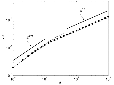
Figure 4: Volatility of returns as a function of lag time $\Delta$. Symbols show the results of numerical simulation; dotted line is the analytical expression (46); dashed line is the small-$\Delta$ approximation (47); solid lines show power-laws with exponent $0.5$ (large lags), and $0.77$ (small lags), as fitted to empirical data in [7].

found by numerical simulation is plotted as a function of the lag $\Delta$ in Fig. 4 (filled circles). The parameter $k$ is chosen as $k=500$, in order to closely match the empirical $\Delta=1$ volatility value as shown in Fig. 3(c) of [6]. Also shown in Fig. 4 is the analytical result (46), plotted as a dotted line, which confirms that the numerical method closely reproduces the exact results of section 4. The dashed line in Fig. 4 is the small-lag approximation (47), and shows that the super-diffusive region of volatility (for lags under 10 minutes) is well-matched by the logarithmic-corrected quadratic power law in $\Delta$. Analysis of the empirical data frequently leads to fitting the super-diffusive volatility with a power-law, with exponents in the range 0.67 [6] to 0.77 [7]. At longer lags ($\Delta>10$), random walk behavior ($\text{vol}\sim\sqrt{\Delta}$) is observed in all studies, and reproduced in our model as shown following equation (49). The solid lines in Fig. 4 show power-law scalings, with exponents 0.77 (for $\Delta<10$), and 0.5 (for $\Delta\gg 10$), which are found in [7] to match the S&P500 volatility. Clearly these scalings also match the results of our model quite well, indicating that the model predictions behave similarly to the empirical volatility curve. Indeed, our result (47) predicts that a log-corrected quadratic fit should be superior to the power-law fits used in [6, 7]. Testing this prediction requires higher frequency analysis of the empirical market data.

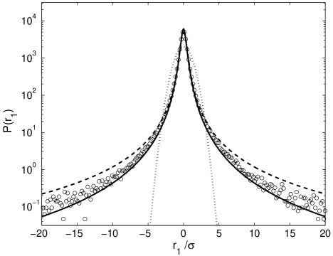
Figure 5: Probability distribution function of 1-minute returns from numerical simulation (symbols). Dashed line is the Lévy distribution fitted to empirical data in [5]; solid line is the Lagrangian velocity PDF (31); dashed line is a Gaussian distribution with same variance as the data.

The probability distribution function (PDF) of the one-minute returns, $r_{1}(t)$, is plotted in Fig. 5. Open circles are from numerical simulations, and are well-fitted by the Lagrangian velocity PDF (31), up to high returns values. Note the returns are normalized by their standard deviation $\sigma\equiv\text{vol}(1)=2\times 10^{-4}$. The Gaussian distribution with this standard deviation is plotted with the dotted line: note the higher-than-Gaussian central peak of the model results, and the fatter tails. Fig. 5 is remarkably similar to Fig. 2 of [5], which shows the one-minute returns PDF from the S&P500. Indeed, in [5] it is demonstrated that the empirical results are well-fitted near the center of the distribution by a Lévy stable distribution with index $\alpha=1.4$, and so in Fig. 5 we also show this distribution (dashed line), with scale factor chosen to match the peak value of the numerical distribution. Comparison with Fig. 2 of [5] shows that our numerical simulation returns have a very similar distribution to the S&P500 data, at least within $\pm 10\sigma$.

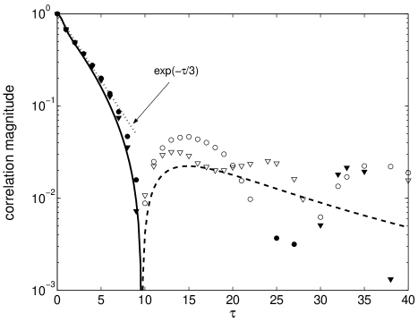
Figure 6: Magnitude of the correlation function of 1-minute returns, as a function of separation time $\tau$. Numerical results from two realizations are shown (circles and triangles), with the analytical form (34) (solid and dashed lines). Negative correlation values are shown with open symbols and dashed line. The dotted line shows $\exp(-\tau/3)$ for comparison.

In Fig. 6 we consider the correlation function of the one-minute returns over a separation time $\tau$, normalized by the volatility:

$$\frac{\left<r_{1}(t)r_{1}(t+\tau)\right>}{\left<r_{1}(t)^{2}\right>}.$$ (59)

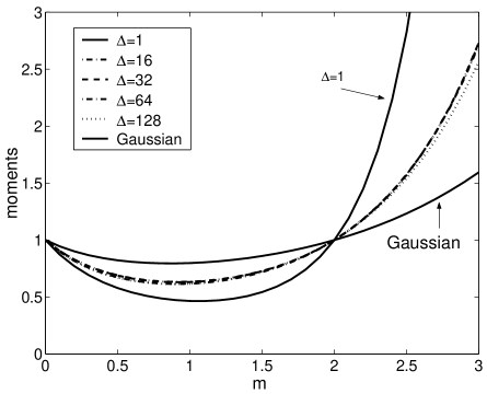
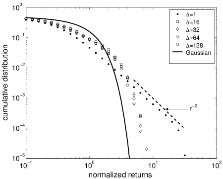
Figure 8: (a) Moments of the normalized returns, for lag times $\Delta=1$, 16, 32, 64, and 128 minutes. (b) Corresponding cumulative distribution functions, with the dashed line showing a power-law with exponent -2.

As this quantity has both positive and (small) negative values, we plot its absolute value on a log-linear scale. Statistical scatter causes some uncertainty in these numerical results, so the results of two different realizations (circles and triangles, respectively) are shown. According to (36) and (45), the returns correlation is negative for $\tau\gg 10$ minutes, which is confirmed by plotting the analytical result (34): this is shown as a solid line where the correlation is positive, and a dashed line where it is negative. The numerical simulation results match the analytical form well for $\tau<10$ minutes, but degrade in quality when the correlation is negative. It is possible that more advanced numerical simulation methods such as Fourier-Wavelet [31] could alleviate this problem. Note filled symbols show positive numerical correlation values, with open symbols for negative values. The rapid decay of the correlation from $\tau=0$ to $\tau=10$ minutes (see dotted line showing $\exp(-\tau/3)$ for comparison) is reminiscent of that found in S&P500 data, see Fig. 3(a) of [6] and Fig. 8(a) of [28]. Unlike our model results, however, the empirical correlation does not exhibit negative values but instead reaches a “noise level” around $3\times 10^{-3}$, where it flattens out without discernable structure. Our model suggests that it might be fruitful to search for evidence of negative correlations in the empirical data, which may currently be screened by the noise level.

The correlation function of the absolute value of one-minute returns (normalized to unity at zero separation) is

$$\frac{\left<\left|r_{1}(t)r_{1}(t+\tau)\right|\right>-\left<\left|r_{1}(t)\right|\right>^{2}}{\left<\left|r_{1}(t)^{2}\right|\right>-\left<\left|r_{1}(t)\right|\right>^{2}}.$$ (60)

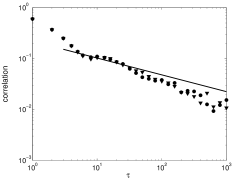
Figure 7: Correlation function of absolute 1-minute returns, as a function of separation time $\tau$. Numerical results from two realizations are shown (circles and triangles). The solid line is a power-law scaling as (51).

From empirical data, this is known to have a slow power-law decay with $\tau$, with exponent of approximately $-1/3$, see Fig. 3(b) of [6] and Fig. 8(b) of [28]. The analytical result (51) for the present model indicates that a similar power-law form holds, indeed this is what motivated our choice of parameter $\beta=1/6$ in (55). Fig. 7 shows numerical results from two separate realizations (circles and triangles), with the solid line showing a power-law decay with exponent $-1/3$. The numerical correlations are all positive, but show a slight deviation from the expected power-law scaling. This may be related to the poor representation of the negative values of the returns correlation in Fig. 6. Comparison with empirical data (Fig. 3(b) of [6] and Fig. 8 (b) of [28]) also shows that the model’s correlation decays faster than that of the S&P500 data for $\tau<10$ minutes.

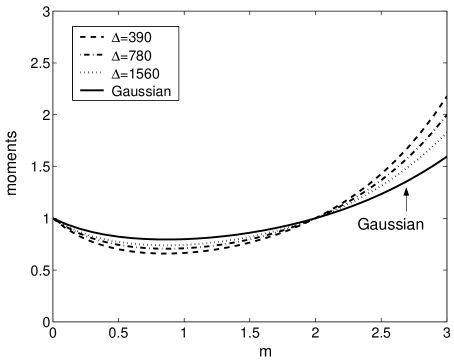
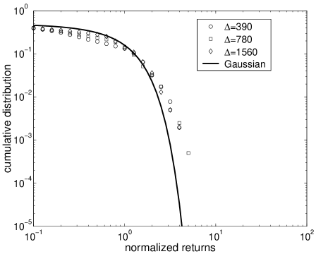
Figure 9: (a) Moments of the normalized returns, for lag times $\Delta=390$, 780, and 1560 minutes. (b) Corresponding cumulative distribution functions.

The non-Gaussian distribution of returns over longer time lags is examined in Figs. 8 and 9, using the methods applied to S&P500 data in Figs. 6 to 8 of [6]. The normalized returns are defined by dividing by the volatility:

$$g_{\Delta}(t)=\frac{r_{\Delta}(t)}{\text{vol}(\Delta)},.$$ (61)

and the moments

$$\left<\left|g_{\Delta}(t)\right|^{m}\right>$$ (62)

of the numerical simulations are plotted in Fig. 8(a) as a function of $m$, for lags of 1, 16, 32, 64, and 128 minutes. The extremely non-Gaussian distribution at $\Delta=1$ minute relaxes to a shape which remains stable up to $\Delta\approx 128$ minutes—note the moments for lags from 16 to 128 minutes are almost indistinguishable in Fig. 8(a). This conclusion is supported by the cumulative distribution of the normalized returns shown in Fig. 8(b). This is very similar to the behavior observed in empirical data, see Fig. 6 of [6], although the model does not produce power-law scaling of the distribution tails (except for the region with exponent -2 for lag $\Delta=1$ minute). The returns distributions eventually converge to a Gaussian distribution, see the corresponding plots for lags of 390, 780, and 1560 minutes (1 to 4 trading days) in Fig. 9. This convergence to Gaussian is somewhat faster that that observed in the S&P500 in [6], where non-Gaussian moments and cumulative distributions persist until approximately 4 days. Our corresponding estimate for the model persistence time (based on the moments in Fig. 8(a)) is 128 minutes, an order of magnitude smaller that the S&P500 value.

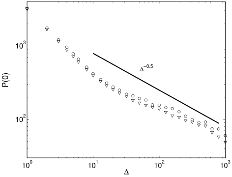
Figure 10: Scaling of the peak $P(0)$ of the stock returns PDF with lag time $\Delta$. Solid line shows a Gaussian scaling, with exponent $-0.5$.

The scaling of the peak $P(0)$ of the PDF of stock price returns $S(t+\Delta)-S(t)$ was examined in [5] for S&P500 data. A power-law scaling of $P(0)$ with lag was discovered, with exponent $-0.7$. In Fig. 10 we mimic this study, generating the time series $S(t)$ from $x(t)$ in order to calculate the stock price return. Results are shown from two separate realizations, along with a line indicating Gaussian scaling of exponent $-1/2$. It is clear that, unlike the S&P500 returns, the model $P(0)$ does not scale as a single power-law with $\Delta$, although it appears to approach the Gaussian scaling at the highest lags.

7 Conclusion

We have proposed a new model for the fluctuations of stock prices, in which the rate of change of the log price is randomly dependent upon both time and the current price, see equation (7). This is a very general modelling concept, with the attractive feature that Gaussian Eulerian fields may give non-Gaussian Lagrangian statistics in the observable data, i.e. the time series of returns. As noted in section 5, Monte-Carlo simulations of equation (7) can be used to find the model predictions for any random field. In this paper we focus on a special case, the $\epsilon\rightarrow 0$ limit of a single-scale random field, for which exact analytical results are obtainable, and for which numerical simulations are particularly efficient.

Our main analytical results are the expression (42) for the Lagrangian velocity correlation $L(t)$ in terms of the given Eulerian field correlation $R(t)$, and the quadrature formulas (34) and (46) giving the correlation function and volatility of the returns. Numerical simulations of stock price time series are efficiently performed using equation (56), and allow us to examine features not amenable to exact analysis.

We find that several of the important empirical stylized facts (i)-(iv) listed in the Introduction are reproduced by our model, using the correlation function (55) for computational convenience. The parameter values $k$ and $T$ are chosen by comparing the model’s volatility to the data in Fig. 3(c) of [6]. With reference to the stylized facts listed in section 1, the results of the single-scale random field model may be summarized as follows.

• Model returns are non-Gaussian, with fat tails and the center of the distribution well-fitted by the Lévy distribution used in [5]. The tails of the cumulative distributions of model returns do not, however, have the power-law scaling found in [6]. The normalized model returns distributions exhibit a slow return toward Gaussian, on timescales an order of magnitude longer than the characteristic time of $R(t)$. However, these timescales are an order of magnitude smaller those found for the convergence to Gaussian in the S&P500 returns in [6].

• The correlation function of model returns decays quickly (similar to exponentially) over a short timescale. Following the fast decay, the correlation becomes negative, with magnitude decaying more slowly to zero. Although the fast decay for lags under 10 minutes is very similar that found for the S&P500 in [6], the empirical correlation function does not reach negative values, rather remaining at a constant “noise level”. Whether this noise level could be masking negative correlation values as predicted by the model is a question requiring further extensive analysis of market data.

• The volatility of the model returns grows diffusively for lag times longer than 10 minutes. The super-diffusive volatility at higher frequencies (shorter lags) is actually due to a logarithmic correction to power-law growth (47), but for the range of lags examined in [6, 7] it matches well to a super-diffusive power-law. Higher frequency data is needed to determine which form best fits the actual stock market volatility.

• Our model does not have a simple scaling of $P(0)$ with lag, in contrast to the case of S&P500 prices as demonstrated in Fig. 1 of [5].

In summary, the single-scale random field model yields time series which have many (but not all) of the important properties of empirical data. The model gives an appealingly intuitive picture of the causes of non-Gaussian behavior in markets, and provides a simple algorithm for generating time series with many market-like features. We anticipate that this algorithm will prove particularly useful in Monte-Carlo simulations to determine prices of options and derivatives when non-Gaussian returns are particularly important [3, 4].

The concept of modelling stock prices by motion in a random field is quite general, and suggests many directions for further work. Among these are:

• Examining the consequences of such models for the pricing of options and derivatives, and comparison with the standard Black-Scholes (random-walk-based) results.

• Further market data analysis, to determine if there is any evidence of the negative correlation or log-corrected volatility scaling discussed in (ii) and (iii) above.

• Finding a microeconomic basis for the random field model (7), possibly based on the actions of multiple independent agents [26, 27].

• Numerical simulations of (7) for more general field correlations $S(x)$ and different $\epsilon$ values, to determine which of the results detailed here are universal features of motion in random fields, and which are specific to the single-scale, $\epsilon\rightarrow 0$ case analyzed here.

8 Acknowledgements

The author gratefully acknowledges helpful discussions with John Appleby and Paul O’Gorman. This work is supported by funding from a Science Foundation Ireland Investigator Award 02/IN.1/IM062, and from the Faculty of Arts Research Fund, University College Cork.

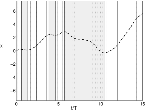
Figure 1: Motion of a stock tracer in a random field which depends only on time, as in (5). Shaded areas and dotted contour lines indicate negative values of $u_{c}(t)$.

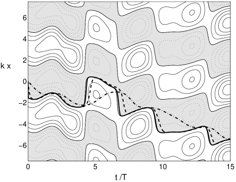
Figure 3: Motion of stock tracers in a single-scale random field. See Fig. 2 for description of line types.

References

- [1] L. Bachelier, Ann. Sci. Ec. Norm. Sup. 3, 21 (1900).
- [2] P. A. Samuelson, in The Random Character of Stock Market Prices, edited by P. H. Cootner (MIT Press, Cambridge, 1964), pp. 506.
- [3] J. C. Hull, Options, futures, and other derivatives (Prentice Hall, London, 2003).
- [4] J. Y. Campbell et al., The econometrics of financial markets (Princeton University Press, Princeton, 1997).
- [5] R. N. Mantegna and H. E. Stanley, Nature 376, 46 (1995).
- [6] P. Gopikrishnan et al., Phys. Rev. E 60, 5305 (1999).
- [7] J. Masoliver, M. Montero, and J. M. Porrà, Physica A 283, 559 (2000).
- [8] N. G. Van Kampen, Stochastic Processes in Physics and Chemistry (Elsevier, Amsterdam, 1992).
- [9] L. Arnold, Stochastic Differential Equations: Theory and Applications (Wiley, New York, 1974).
- [10] B. B. Mandelbrot, J. Bus. 36, 394 (1963).
- [11] R. N. Mantegna and H. E. Stanley, Phys. Rev. Lett. 73, 2946 (1994).
- [12] R. F. Engle, Econometrica 50, 987 (1982).
- [13] T. Bollerslev, R. Y. Chou, and K. F. Kroner, J. Economentrics 52, 5 (1992).
- [14] O. E. Barndorff-Nielsen and N. Shephard, J. R. Statist. Soc. B 63, 167 (2001).
- [15] J. Masoliver, M. Montero, and G. H. Weiss, Phys. Rev. E 67, 021112 (2003).
- [16] R. N. Mantegna and H. E. Stanley, Physica A 254, 77 (1998).
- [17] R. N. Mantegna and H. E. Stanley, Physica A 274 216 (1999).
- [18] J. P. Gleeson and D. I. Pullin, Phys. Fluids, to appear.
- [19] J. B. Witkoskie, S. Yang, and J. Cao, Phys. Rev. E 66, 051111 (2002).
- [20] A. M. Balk, J. Fluid Mech. 467, 163 (2002).
- [21] R. H. Kraichnan, Phys. Fluids 13, 22 (1970).
- [22] W. D. McComb, The Physics of Fluid Turbulence (Oxford University Press, Oxford, 1990).
- [23] C. L. Zirbel, Adv. Appl. Prob. 33, 810 (2001).
- [24] M. Vlad et al., Phys. Rev. E 63 066304 (2001).
- [25] J. P. Gleeson, Phys. Rev. E. 66, 038301 (2002).
- [26] T. Lux and M. Marchesi, Nature 397 498 (1999).
- [27] J. A. D. Appleby, Int. J. Theor. Appl. Fin. 3, 491 (2000).
- [28] Y. Liu et al., Phys. Rev. E 60, 1390 (1999).
- [29] R. E. O’Malley, Singular perturbation methods for ordinary differential equations (Springer-Verlag, New York, 1991).
- [30] J. P. Gleeson, Phys. Rev. E, 65, 037103 (2002).
- [31] A. J. Majda and P. R. Kramer, Phys. Rep. 314, 237 (1999).