Shot noise spectrum of superradiant entangled excitons

Abstract

The shot noise produced by tunneling of electrons and holes into a double dot system incorporated inside a p-i-n junction is investigated theoretically. The enhancement of the shot noise is shown to originate from the entangled electron-hole pair created by superradiance. The analogy to the superconducting cooper pair box is pointed out. A series of Zeno-like measurements is shown to destroy the entanglement, except for the case of maximum entanglement.

I Introduction

Quantum entanglement has become one of the most important issues since the rapid developments in quantum information science 1 . Much research has been devoted to studying entanglement as induced by a direct interaction between the individual subsystems 2 . Very recently, a lot of attention has been focused on reservoir-induced entanglement 3 with the purpose to shed light on the generation of entanglement, and to better understand quantum decoherence.

Furthermore, shot noise 4 has been identified as a valuable indicator of particle entanglement in transport experiments.5 A well studied example is the doubling of the full shot noise in S-I-N tunnel junctions6 , where N is a normal metal, S stands for a superconductor, and I is an insulating barrier. The origin of this enhancement comes from the break-up of the spin-singlet state, which results in a quick transfer of two electrical charges.

In this paper, we demonstrate how the dynamics of entangled excitons formed by superradiance can be revealed from the observations of current fluctuations. A doubled zero-frequency shot noise is found for the case of zero subradiant decay rate. We relate the particle noise to photon noise by calculating the first order photon coherence function. Furthermore, strong reservoir coupling acts like a continuous measurement, which is shown to suppress the formation of the entanglement, except for the state of maximum entanglement. These novel features imply that our model provides a new way to examine both the bunching behavior and a Zeno-like effect of the reservoir induced entanglement.

II Double Dot Model

The effect appears in double quantum dots embedded inside a p-i-n junction7 . It involves superradiant and subradiant decay through two singlet and triplet entangled states, $\left|S_{0}\right\rangle=\frac{1}{\sqrt{2}}(\left|U_{1}\right\rangle-\left|U_{2}\right\rangle)$ and $\left|T_{0}\right\rangle=\frac{1}{\sqrt{2}}(\left|U_{1}\right\rangle+\left|U_{2}\right\rangle)$, and one ground state $\left|D\right\rangle=\left|0,0;0,0\right\rangle$, where $\left|U_{1}\right\rangle=\left|e,h;0,0\right\rangle$ ( $\left|U_{2}\right\rangle=\left|0,0;e,h\right\rangle$ ) represents one exciton in dot 1 (2). Electron and hole reservoirs coupled to both dots have chemical potentials such that electrons and holes can tunnel into the dot. For the physical phenomena we are interested in, the current is assumed to be conducted through dot 1 only (Fig. 1). Therefore, the exciton states $\left|0,0;e,h\right\rangle$ (in dot 2) can only be created via the exciton-photon interactions.

Figure 1: Schematic view of the structure.

The exciton-photon coupling is described by an interaction Hamiltonian

$$H_{I} = \sum_{\mathbf{k}}\frac{1}{\sqrt{2}}g\{D_{\mathbf{k}}b_{\mathbf{k}}[(1+e^{i\mathbf{k}\cdot\mathbf{r}})\left|S_{0}\right\rangle\left\langle D\right|$$ (1)

$$+(1-e^{i\mathbf{k}\cdot\mathbf{r}})\left|T_{0}\right\rangle\left\langle D\right|]+H.c.\},$$

where $b_{\mathbf{k}}$ is the photon operator, $gD_{\mathbf{k}}$ is the coupling strength, $\mathbf{r}$ is the position vector between the two quantum dots. Here, $g$ is a constant with the unit of the tunneling rate. The dipole approximation is not used in our calculation since we keep the full $e^{i\mathbf{k}\cdot\mathbf{r}}$ terms in the Hamiltonian. The coupling of the dot states to the electron and hole reservoirs is described by the standard tunnel Hamiltonian

$$H_{V}=\sum_{\mathbf{q}}(V_{\mathbf{q}}c_{\mathbf{q}}^{\dagger}\left|0\right\rangle\left\langle U_{1}\right|+W_{\mathbf{q}}d_{\mathbf{q}}^{\dagger}\left|0\right\rangle\left\langle D\right|+H.c.),$$ (2)

where $c_{\mathbf{q}}$ and $d_{\mathbf{q}}$ are the electron operators in the left and right reservoirs, respectively, and $\left|0\right\rangle=\left|0,h;0,0\right\rangle$ denotes one-hole state in dot 1. $V_{\mathbf{q}}$ and $W_{\mathbf{q}}$ couple the channels $\mathbf{q}$ of the electron and the hole reservoirs. Here we have neglected the state $\left|e,0;0,0\right\rangle$ for convenience. This can be justified by fabricating a thicker barrier on the electron side so that there is little chance for an electron to tunnel in advance 8 .

III Rate Equations and Noise Spectrum

The rates $\Gamma_{U}$ (electron reservoir) and $\Gamma_{D}$ (hole reservoir) for tunneling between the dot and the connected reservoirs can be calculated from $H_{V}$ by perturbation theory. In double quantum dots, decay of the excited levels is governed by collective behavior, i.e. superradiance and subradiance. The corresponding decay rates for the state $\left|S_{0}\right\rangle$ and $\left|T_{0}\right\rangle$ can be obtained from $H_{I}$ and are denoted by $g^{2}\gamma_{S}$ and $g^{2}\gamma_{T}$, respectively. We are then in the position to set up the equations of motion for the time-dependent occupation probabilities $n_{j}(t),$ $j=$ $0$, $D,$ $S_{0},T_{0}$, of the double dot states. Together with the normalization condition $\sum_{j}n_{j}(t)=1$, the equations of motion are Laplace-transformed into $z-$space 9 for convenience and read

$$z\hat{n}_{S_{0}}(z) = -ig\left[\hat{p}_{S_{0},D}(z)-\hat{p}_{D,S_{0}}(z)\right]+\Gamma_{U}\left[\frac{1}{z}-\hat{n}_{S_{0}}(z)-\hat{n}_{T_{0}}(z)-\hat{n}_{D}(z)\right],$$

$$z\hat{n}_{T_{0}}(z) = -ig\left[\hat{p}_{T_{0},D}(z)-\hat{p}_{D,T_{0}}(z)\right]+\Gamma_{U}\left[\frac{1}{z}-\hat{n}_{S_{0}}(z)-\hat{n}_{T_{0}}(z)-\hat{n}_{D}(z)\right],$$

$$z\hat{n}_{D}(z) = ig\left[\hat{p}_{S_{0},D}(z)-\hat{p}_{D,S_{0}}(z)+\hat{p}_{T_{0},D}(z)-\hat{p}_{D,T_{0}}(z)\right]-\frac{2\Gamma_{D}}{z}\hat{n}_{D}(z).$$ (3)

Here, $p_{S_{0},D}(t)=p_{D,S_{0}}^{\ast}(t)$ and $p_{T_{0},D}(t)=p_{D,T_{0}}^{\ast}(t)$ are off-diagonal matrix elements of the reduced density operator of the double dots, whose Laplace-transformed equations of motion close the set (3):

$$\hat{p}_{S_{0},D}(z) = ig\gamma_{S}\hat{n}_{S_{0}}(z)-\Gamma_{D}\gamma_{S}\hat{p}_{S_{0},D}(z),$$

$$\hat{p}_{T_{0},D}(z) = ig\gamma_{T}\hat{n}_{T_{0}}(z)-\Gamma_{D}\gamma_{T}\hat{p}_{T_{0},D}(z).$$ (4)

Note that in getting above equations, one has to do a decoupling approximation of dot operators and photon operators. This means we are interested in small coupling parameters here, and a decoupling of the reduced density matrix $\widetilde{\rho}(t^{\prime})$ is used : $\widetilde{\rho}(t^{\prime})\approx\rho_{ph}^{0}Tr_{ph}\rho(t^{\prime})$. 9 The stationary tunnel current $I$ can be defined as the change of the occupation of $n_{D}(t)$ for large times $t$ and is given by

$$I\equiv\lim_{t\to\infty}ig\left[p_{S_{0},D}(t)-p_{D,S_{0}}(t)+p_{T_{0},D}(t)-p_{D,T_{0}}(t)\right],$$ (5)

where we have set the electron charge $e=1$ for convenience.

In a quantum conductor in nonequilibrium, electronic current noise originates from the dynamical fluctuations of the current being away from its average. To study correlations between carriers, we relate the qubit dynamics with the hole reservoir operators by introducing the degree of freedom $n$ as the number of holes that have tunneled through the hole-side barrier and write

$$\overset{\cdot}{n}_{0}^{(n)}(t) = -\Gamma_{U}n_{0}^{(n)}(t)+\Gamma_{D}n_{D}^{(n-1)}(t),$$

$$\overset{\cdot}{n}_{S_{0}}^{(n)}(t) = \frac{\Gamma_{U}}{2}n_{0}^{(n)}(t)+ig(p_{S_{0},D}^{(n)}(t)-p_{D,S_{0}}^{(n)}(t)),$$

$$\overset{\cdot}{n}_{T_{0}}^{(n)}(t) = \frac{\Gamma_{U}}{2}n_{0}^{(n)}(t)+ig(p_{T_{0},D}^{(n)}(t)-p_{D,T_{0}}^{(n)}(t)),$$

$$\overset{\cdot}{n}_{D}^{(n)}(t) = -\Gamma_{D}n_{0}^{(n)}(t)-ig(p_{S_{0},D}^{(n)}(t)-p_{D,S_{0}}^{(n)}(t)$$ (6)

$$+p_{T_{0},D}^{(n)}(t)-p_{D,T_{0}}^{(n)}(t)).$$

Eqs. (6) allow us to calculate the particle current and the noise spectrum from $P_{n}(t)=n_{0}^{(n)}(t)+n_{S_{0}}^{(n)}(t)+n_{T_{0}}^{(n)}(t)+n_{D}^{(n)}(t)$ which gives the total probability of finding $n$ electrons in the collector by time $t$. In particular, the noise spectrum $S_{I_{D}}$ can be calculated via the MacDonald formula 10 .

$$S_{I_{D}}(\omega)=2\omega e^{2}\int_{0}^{\infty}dt\sin(\omega t)\frac{d}{dt}[\left\langle n^{2}(t)\right\rangle-(t\left\langle I\right\rangle)^{2}],$$ (7)

where $\frac{d}{dt}\left\langle n^{2}(t)\right\rangle=\sum_{n}n^{2}\overset{\cdot}{P_{n}}(t)$. Solving Eqs. (6) and (3), we obtain

$$S_{I_{D}}(\omega)=2eI\{1+\Gamma_{D}[\hat{n}_{D}(z=-i\omega)+\hat{n}_{D}(z=i\omega)]\}.$$ (8)

In the zero-frequency limit, Eq. (8) reduces to

$$S_{I_{D}}(\omega=0)=2eI\{1+2\Gamma_{D}\frac{d}{dz}[z\hat{n}_{D}(z)]_{z=0}\},$$ (9)

which is analogous to a recent calculation of noise in dissipative, open two-level systems AB03 .

IV Results

IV.1 Current Noise

To display the dependence of carrier correlations on the dot distance $d$, Fig. 2 shows the result for zero-frequency noise $S_{I_{D}}(\omega=0)$ as a function of the inter-dot distance. In plotting the figure, the tunneling rates, $\Gamma_{U}$ and $\Gamma_{D}$, are assumed to be equal to $0.1\gamma_{0}$ and $\gamma_{0},$ respectively. Here, a value of 1/1.3ns for the free-space quantum dot decay rate $\gamma_{0}$ is used in our calculations 11 . As shown in Fig. 2, the Fano factor

$$F\equiv\frac{S_{I_{D}}(0)}{2e\langle I\rangle}$$

is enhanced by a factor of 2 as the dot distance $d$ is much smaller than the wavelength ($\lambda$) of the emitted photon. To explain this enhancement, we approximate the Fano factor in the limit of small subradiant decay rate, i.e.

$$g^{2}\gamma_{S}\ll\Gamma_{U}<\Gamma_{D}\approx g^{2}\gamma_{T},$$

where we obtain

$$\frac{S_{ID}(0)}{2e\langle I\rangle}\approx 2-2g^{2}\gamma_{S}[\frac{1}{g^{2}\gamma_{T}}+3(\frac{1}{\Gamma_{D}}+\frac{1}{\Gamma_{U}})+\frac{2\Gamma_{D}}{g^{2}}].$$ (10)

This is analogous to the case of the single electron transistor near a Cooper pair resonance as discussed recently by Choi and co-workers 12 . In their calculations, the Fano factor is expressed as $\frac{S(0)}{2e\langle I\rangle}=2-\frac{8E_{J}^{2}(E_{J}^{2}+2\Gamma^{2})}{(3E_{J}^{2}+\Gamma^{2}+4\varepsilon^{2})^{2}}.$ In the strong dephasing limit ($E_{J}\ll\Gamma$, where $E_{J}$ is the Josephson coupling energy), the zero-frequency shot noise is also enhanced by a factor of 2. Since the doubled shot noise in Josephson junction is attributed to the bunching behavior of Cooper pairs (in singlet state), we then conclude the enhancement in our system is also due to the entanglement induced by the photon reservoir.

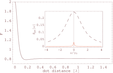
Figure 2: Fano factor as a function of inter-dot distance. The vertical and horizontal units are $\frac{S_{I_{D}}(0)}{2eI}$ and $\lambda$, respectively. The inset shows the value of $S_{ph}(\omega)$ is equal to that of one-dot limit for $d\rightarrow\infty$ (dashed line), while it approaches zero noise as $d=0.005\lambda$ (red line).

IV.2 Photon Noise

It is worthwhile to compare the current noise with the photon noise generated by the collective decay of the double dot excitons. In order to do so, we have calculated the power spectrum of the fluorescence spectrum13 , which can be expressed as

$$S_{ph}(\omega)=\frac{1}{\pi}\mathop{\mathrm{R}e}\int_{0}^{\infty}G^{(1)}[\tau]e^{i\omega\tau}d\tau,$$ (11)

where $G^{(1)}[\tau]$ is the first order coherence function and reads

$$G^{(1)}[\tau] \propto \left|1+e^{i2\pi d/\lambda}\right|^{2}\left\langle p_{S_{0},D}(0)p_{D,S_{0}}(\tau)\right\rangle$$ (12)

$$+\left|1-e^{i2\pi d/\lambda}\right|^{2}\left\langle p_{T_{0},D}(0)p_{D,T_{0}}(\tau)\right\rangle.$$

The two time-dependent correlation functions in the above equation can be calculated from the quantum regression theorem, and the numerical result of $S_{ph}(\omega)$ is shown explicitly in the inset of Fig. 2. As can be seen, the value of $S_{ph}(\omega)$ is equal to that of the one-dot case for $d\rightarrow\infty$ (dashed line), while it approaches zero as $d=0.005\lambda$ (red line). In the limit of $d=0$, one observes no photon emission from the double dot system since the exciton is now in its maximum entangled state and does not decay. This feature implies that photon noise is suppressed by the bunching of excitons, and its behavior is opposite to that for the electronic case 14 .

IV.3 Noise and Measurement

Now we investigate how the measurement affects the shot noise spectrum. In the usual Zeno paradox 15 , a two-level system (qubit) is completely frozen under a series of measurements, whose time interval $\Delta t$ is much smaller than the memory time of the reservoir. In our model, the presence of the exciton state can be viewed as the excited state, and whether or not the next hole can tunnel in is determined by the occupation of this state. Similar to the quantum Zeno effect, the tunneling of holes at the hole-side tunneling rate $\Gamma_{D}$ can be thought as a continuous measurements. The ”interval time” $\Delta t$ is then inversely proportional to $\Gamma_{D}.$ Fig. 3 represents the effects of measurements on the frequency-dependent shot noise spectrum. The numerical results for the tunneling rate $\Gamma_{D}=20$ $\gamma_{0}$ and $\Gamma_{D}=$ $\gamma_{0}$ are demonstrated by solid and dashed curves, respectively. If the subradiant decay rate is set to zero, one obtains the doubled shot noise as mentioned above. Without superradiance, the values of the Fano factor are always below unity as shown by the right inset of Fig. 3. An interesting feature is that the half-width of the spectrum is narrowed for strong measurements ($\Gamma_{D}=20$ $\gamma_{0}$). If one increases the electron-side tunneling rate $\Gamma_{U}$, there exists no such behavior. This implies that the effective decay rate is reduced in the presence of strong measurements.

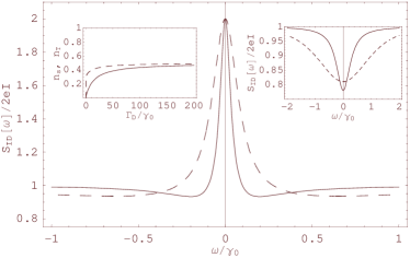
Figure 3: Effect of measurements on current noise  $S_{ID}(\omega)$ ( ”maximum” superradiance, $g^{2}\gamma_{T}=2g^{2}\gamma_{0}$ , $g^{2}\gamma_{S}=0$). Solid and dashed lines correspond to $\Gamma_{D}=20$ $\gamma_{0}$ and $\Gamma_{D}=$ $\gamma_{0}$ , respectively. Right inset : the case of no superradiance. Left inset : expectation value of the excited states $\left\langle n_{S}\right\rangle$ and $\left\langle n_{T}\right\rangle$ as a function of $\Gamma_{D}.$

To investigate thoroughly the underlying physics, we plot the expectation value of the excited states $\left\langle n_{S}\right\rangle$ and $\left\langle n_{T}\right\rangle$ as a function of $\Gamma_{D}$ in the left inset of Fig. 3. One clearly finds the occupation probabilities grow with increasing $\Gamma_{D}$, and both of them approaches the value of $\frac{1}{2}$. This not only means the measurements tend to localize the exciton in its excited state 16 , but also tells us the entanglement is destroyed under the strong measurements. However, in the limit of no subradiance ($g^{2}\gamma_{S}=0$), the occupation probability of the singlet state is always equal to one, i.e. maximum entanglement is robust against strong measurements. This is because once the maximum entangled state is formed, the total probability in the excited states is also maximum. Strong measurements on the ground state $\left|D\right\rangle$ have no influence on the singlet entangled state.

V Discussion and Conclusion

A few remarks about experimental realizations of the present model should be mentioned here. One should note that biexciton and charged-exciton effects are not included in our present model. Inclusion of these additional states is expected to suppress the enhancement of the shot noise, i.e. degrees of entanglement. However, this can be controlled well by limiting the value of bias voltage so that only the ground-state exciton is present 17 . To produce the maximum entangled state, one can also incorporate the device inside a microcavity 18 . There are two advantages of this design: The maximum entanglement can be generated even for remote separation of the two dots, and Forster process 19 is avoided at this distance.

As for the problem of decoherence due to interactions with phonons, recent experimental data have shown that the exciton-phonon dephasing rate is smaller than the radiative decay one in a quantum dot. This means that due to the discrete energy level scheme in a quantum dot, the effect of phonon-bottleneck tends to suppress the exciton-phonon interaction 20 . Although the present model describes tunneling of electrons and holes into semiconductor quantum dots, the whole theory can be applied to electron tunneling through coupled quantum dots which are interacting via a common phonon environment 21 .

In conclusion, we have demonstrated that the shot noise of superradiant entangled excitons is enhanced by a factor of two as compared to the poissonian value. This enhancement was attributed to exciton entanglement, induced by the electromagnetic field (common photon reservoir), and an analogy to the Cooper pair box was made. Second, we found the relaxation behavior of the qubits in the presence of strong measurements, and the Zeno-like effect tends to destroy the entanglement and localize the qubits in the excited states.

This work is supported partially by the National Science Council, Taiwan under the grant number NSC 92-2120-M-009-010.

References

- (1) C. H. Bennett and D. P. DiVincenzo, Nature (London) 404, 247 (2000); T. Pellizzari et al., Phys. Rev. Lett. 75, 3788 (1995); J. I. Cirac and P. Zoller, Phys. Rev. Lett. 74, 4091 (1995); K. Molmer and A. Sorensen, Phys. Rev. Lett. 82, 1835 (1999).
- (2) A.T. Costa et al., Phys. Rev. Lett. 87, 277901 (2001); W.D. Oliver et al., Phys. Rev. Lett. 88, 037901 (2002); Oliver Gywat et al., Phys. Rev. B 65, 205329 (2002).
- (3) M. S. Kim et al., Phys. Rev. A 65, 040101 (2002); Daniel Braun, Phys. Rev. Lett. 89, 277901 (2002); Fabio Benatti et al., Phys. Rev. Lett. 91, 070402 (2003); R. Ruskov and A. N. Korotkov, Phys. Rev. B 67, 241305 (2003).
- (4) Y. M. Blanter and M. Büttiker, Phys. Rep. 336, 1 ( 2000); C. W. J. Beenakker, Rev. Mod. Phys. 69, 731 (1997).
- (5) P. Samuelsson et al., Phys. Rev. Lett. 91, 157002 (2003); C. W. J. Beenakker et al., Phys. Rev. Lett. 91, 147901 (2003).
- (6) F. Lefloch et al., Phys. Rev. Lett. 90, 067002 (2003).
- (7) O. Benson et al., Phys. Rev. Lett. 84, 2513 (2000).
- (8) In the following calculations, the electron-side tunneling rate is always assumed to be much smaller than the hole-side tunneling rate .
- (9) T. Brandes and B. Kramer, Phys. Rev. Lett. 83, 3021 (1999).
- (10) D. K. C. MacDonald, Rep. Prog. Phys. 12, 56 (1948); D. Mozyrsky et al., Phys. Rev. B 66, 161313 (2002).
- (11) R. Aguado, T. Brandes, cond-mat/0310578 (2003).
- (12) G. S. Solomon et al., Phys. Rev. Lett. 86, 3903 (2001).
- (13) Mahn-Soo Choi et al., Phys. Rev. Lett. 87, 116601 (2001).
- (14) M. O. Scully and M. S. Zubairy, Quantum optics, Cambridge University Press (1997).
- (15) Guido Burkard et al., Phys. Rev. B 61, 16303 (2000).
- (16) B. Misra and E. C. G. Sudarshan, J. Math. Phys. (N.Y.) 18, 756 (1977).
- (17) A. N. Korotkov and D. V. Averin, Phys. Rev. B 64, 165310 (2001); S. A. Gurvitz et al., Phys. Rev. Lett. 91, 066801 (2003).
- (18) Z. Yuan et al., Science 295, 102 (2002).
- (19) Y. N. Chen et al., Phys. Rev. Lett. 90, 166802 (2003).
- (20) L. Quiroga and N. Johnson, Phys. Rev. Lett. 83, 2270 (1999).
- (21) N. H. Bonadeo et al., Phys. Rev. Lett. 81, 2759 (1998); D. Birkedal et al., Phys. Rev. Lett. 87, 227401 (2001); P. Borri et al., Phys. Rev. Lett. 87, 157401 (2001).
- (22) T. Vorrath and T. Brandes, Phys. Rev. B 68, 035309 (2003).