Topological Spin Pumps

Abstract

We have established semiclassical kinetic equations for various spin correlated pumping phenomena incorporating adiabatic spin rotation in wave functions. We employ this technique to study topological pumps and illustrate spin pumping in a few models where various spin configurations or topological motors drive adiabatic pumps. In the Rashba model we find that a topological spin pump is driven by a meron with positive one half skyrmion charge, the size of which can be controlled by external applied gates or Zeeman fields. In the Dresselhaus model on the other hand, electron spins are pumped out by a negative meron. We examine the effects of Zeeman fields on topological spin pumping and responses of Fermi seas in various topological pumps. The phenomena of topological pumping are attributed to the beam splitting of electrons in the presence of spin rotation, or topological Stern-Gerlach splitting and occur in a transverse direction along which charge pumping currents might either vanish or are negligible. The transport equations established here might also be applied to the studies of anomalous Hall effect and spin Hall effect as demonstrated in one of the appendices. All results are obtained in an adiabatic expansion where the adiabaticity conditions in Eqs.(56),(67),(151),(152) are satisfied.
PACS number: 03.65. Vf, 73.43.-f

I Introduction

Adiabatic transport of electrons or quantum pumping which is nearly reversible has been one of very promising means to manipulate coherent wave packets in the extreme quantum limit. In the presence of periodic adiabatic perturbations, a net charge can be transferred across a quantum structure during each period which is independent of frequencies of external perturbations and which represents a DC current induced by adiabatic perturbations. This phenomenon was first observed in an early work on transport of edge electrons in quantum Hall states [1]. But general solutions to this problem were provided in Ref.[2] where conditions of quantized charge transport were established. The robustness of quantized transport with respect to disorder potentials and applications to quantum Hall effects were later on studied in a series of works[3].

The absence of dissipation during the adiabatic process is evident if perturbations are applied to a closed quantum structure with nontrivial topology such as a mesoscopic ring or torus. If one further assumes that the electron spectrum is discrete and the external frequency is incommensurate with energy gaps in the spectrum, then no resonance absorption can occur and quantum states evolve via unitary transformation which conserves the entropy. The absence of entropy production in the adiabatic process is therefore a natural consequency of a pure state evolution which has been known for a while.

For a quantum structure with continuous spectra either because of contact with leads in a mesoscopic limit or more generally because of thermal broadening, it is more convenient to introduce one-particle density matrices to describe the evolution of quantum systems. The adiabaticity can be achieved when the frequency of applied perturbations is lower than various relaxation rates characterizing the dynamics of one-particle density matrix. The issue of entropy production in this case however hasn’t been fully addressed and is less well understood. Nevertheless, it is widely appreciated that dissipation involved in adiabatic transport in this limit should also be smaller than that due to a transport current with biased voltages applied.

Given the obvious advantage of the adiabatic charge transport, in this article I intend to generalize the idea to adiabatic spin transport. I will address the issue of spin pumping in both limits which can be easily achieved in laboratories and limits which are theoretically exciting but might not be as easy to be realized in solid state structures. Particularly, I will propose a novel spin pumping mechanism which is based on the topological beam splitting of electrons instead of the usual Zeeman splitting. Special classes of models are introduced to facilitate discussions on topological spin pumping. At the end, I will compare the efficiency of different spin pumping schemes.

One obvious mean to pump spin out of the system is to adiabatically transfer polarized electrons in quantum structures. During the adiabatic transport, the currents carried by spin-up and spin-down electrons have an asymmetric part and therefore electrons pumped out of the structures also carry net spins. This standard scheme is reviewed in section III.

In section IV, I discuss the phenomena of topological beam splitting in details. Particularly, I demonstrate that spin rotation in either real-space ($X$-space) or in Fermi seas leads to transverse motion of electrons. In section V and VI, I investigate topological spin pumping due to spin rotation either in the $X$-space or in Fermi seas. In both cases, spin-up and spin-down electrons though both are electrically negatively charged, carry certain topological charges with opposite signs. As consequencies, spin-up and spin-down electrons can be split because of opposite topological transverse forces, an analogy of splitting of electrons and positrons in an orbital magnetic field. I would like to refer this kind of beam splitting as topological Stern-Gerlach splitting (TSGS) to contrast the usual Stern-Gerlach splitting of spin-up and -down particles in atomic physics. In this article I focus on the origin of this phenomenon and basics features. I plan to present a practical design of a topological spin pump in a subsequent paper.

Finally, in connection with topological spin pumping to be discussed in the article, it is worth mentioning a few recent works on anomalous Hall effects and spin injection where the topology of Hilbert spaces plays a paramount role. In Ref.[7], the authors pointed out that interactions between conduction electrons and background skyrmion configurations activated in magnetite might be responsible for the sign and temperature dependence of anomalous Hall effects observed in Ref.[8]. The authors of Ref.[9] meanwhile argued that ${\bf k}$-space Chern-number densities also modify the equation of motion for electrons. The corresponding contributions to the anomalous Hall effect in ferromagnetic semiconductors were further studied in Ref. [10]. Following these works, it is now believed that the anomalous Hall effect can be an intrinsic phenomenon. It is indeed likely to occur when skew-scattering from impurity atoms is absent as proposed by Karplus and Luttinger a while ago[11]. In Ref.[12] the authors have considered intrinsic spin Hall currents in semiconductors; many interesting features have been found. Related discussions can be also found in Ref.[13].

Independently, in a series of illuminating works[14, 15, 16] the authors studied spin injection in semiconductors characterized by the Luttinger Hamiltonian. They have found that singular topological structures in the ${\bf k}$-space as well have fascinating effects on accelerated electrons and lead to important consequencies on spin injection. In Ref.[15], the authors further pointed out possible connection between transverse spin Hall currents and supercurrent in superconductors. The issue of dissipation however is still under debate and remains to be fully understood.

II Kinetic equations for one-particle density matrix

Consider the one-particle density matrix $\rho_{\alpha\beta}({\bf x}^{\prime},{\bf x};t^{\prime},t)$. Subsripts $\alpha,\beta=\pm$ are introduced as spin indices; later in this article I also introduce $\eta,\xi=1,2,..N$ as indices in an $N$-dimensional parameter space; $\mu,\nu=x,y,z$ as indices in the real or momentum spaces. The evolution of one-particle density matrix is determined by the following equation

$$[i\frac{\partial}{\partial t}+i\frac{\partial}{\partial t^{\prime}}]{\rho}_{\alpha\beta}({\bf x}^{\prime},{\bf x};t^{\prime},t)={\cal H}_{\alpha\beta^{\prime}}({\bf x},i\frac{\partial}{\partial{\bf x}};t)\rho_{\beta^{\prime}\beta}({\bf x}^{\prime},{\bf x};t^{\prime},t)-\rho_{\alpha\beta^{\prime}}({\bf x}^{\prime},{\bf x};t^{\prime},t){\cal H}_{\beta^{\prime}\beta}({\bf x}^{\prime},i\frac{\partial}{\partial{\bf x}^{\prime}};t^{\prime}).$$ (1)

To study the transport in a semiclassical limit, one introduces

$${\bf r}=\frac{{\bf x}+{\bf x}^{\prime}}{2},{\bf X}={\bf x}^{\prime}-{\bf x};$$ (2)

$$T=\frac{t+t^{\prime}}{2},\tau=t^{\prime}-t.$$ (3)

Furthermore, one defines a generalized semiclassical density matrix

$$\rho_{\alpha\beta}({\bf k},{\bf r};\omega,T)=\frac{1}{V}\int d{\bf X}d\tau\exp(i{\bf k}\cdot{\bf X}-i\omega\tau)\rho_{\alpha\beta}({\bf r}+\frac{{\bf X}}{2},{\bf r}-\frac{{\bf X}}{2};T+\frac{\tau}{2},T-\frac{\tau}{2})$$ (4)

$V$ is the volume of systems.

In a semiclassical approximation, one obtains the equation of motion for the one-particle density matrix,

$$\frac{\partial\rho_{\alpha\beta}({\bf k},{\bf r};\omega,T)}{\partial T}+[\frac{\partial H_{\alpha\beta^{\prime}}({\bf k},{\bf r};T)}{\partial{\bf k}}\frac{\partial}{\partial{\bf r}}-\frac{\partial H_{\alpha\beta^{\prime}}({\bf k},{\bf r};T)}{\partial{\bf r}}\frac{\partial}{\partial{\bf k}}+\frac{\partial H_{\alpha\beta^{\prime}}({\bf k},{\bf r};T)}{\partial T}\frac{\partial}{\partial\omega}]\otimes\rho_{\beta^{\prime}\beta}({\bf k},{\bf r};\omega,T)$$ (5)

$$=\frac{1}{i}H_{\alpha\beta^{\prime}}({\bf k},{\bf r};T)\tilde{\otimes}\rho_{\beta^{\prime}\beta}({\bf k},{\bf r};\omega,T)+{\cal I}^{C.I.}\rho_{\alpha\beta}({\bf k},{\bf r};\omega,T).$$ (6)

Here

$$A_{\alpha\beta}\otimes B_{\beta\gamma}=\frac{1}{2}[A_{\alpha\beta}B_{\beta\gamma}+B_{\alpha\beta}A_{\beta\gamma}],$$ (7)

$$A_{\alpha\beta}\tilde{\otimes}B_{\beta\gamma}=A_{\alpha\beta}B_{\beta\gamma}-B_{\alpha\beta}A_{\beta\gamma}.$$ (8)

and ${\cal I}^{C.I.}$ is a collision integral operator for elastic (nonmagnetic) scattering processes. ${\bf k}$ and ${\bf r}$ in Eq.6 are variables instead of operators. The gradient expansion which is valid as far as the transport occurs at a scale much larger than the fermi wave length is sufficient for the study of semiclassical phenomena. In all models employed in this article I find the commutator $H\tilde{\otimes}\rho$ in Eq.6 vanishes in the semiclassical approximation.

The charge current ${\bf J}$ and spin current ${\bf J}^{z}$ with spin along ${\bf e}_{z}$ direction are

$${\bf J}({\bf r},T)=\int\frac{d\omega}{2\pi}\frac{d^{3}{\bf k}}{(2\pi)^{3}}\frac{\partial H_{\alpha\beta}({\bf k},{\bf r})}{\partial{\bf k}}\rho_{\beta\alpha}({\bf k},{\bf r};\omega,T),$$ (9)

$${\bf J}^{z}({\bf r},T)=\int\frac{d\omega}{2\pi}\frac{d^{3}{\bf k}}{(2\pi)^{3}}{\bf e}_{z}\cdot{\bf\sigma}_{\alpha\alpha^{\prime}}\frac{\partial H_{\alpha^{\prime}\beta}({\bf k},{\bf r})}{\partial{\bf k}}\rho_{\beta\alpha}({\bf k},{\bf r};\omega,T).$$ (10)

To facilitate discussions on the adiabatic transport, one further separates the one-particle density matrix into symmetric and asymmetric parts ($\rho_{\alpha\beta}^{S,A}$),

$$\rho_{\alpha\beta}({\bf k},{\bf r};\omega,T)=\rho^{S}_{\alpha\beta}({\bf k},{\bf r};\omega,T)+\rho^{A}_{\alpha\beta}({\bf k},{\bf r};\omega,T)$$ (11)

$${\cal I}^{C.I.}\rho^{S}_{\alpha\beta}({\bf k},{\bf r};T)=0,{\cal I}^{C.I.}\rho^{A}_{\alpha\beta}({\bf k},{\bf r};T)=\frac{1}{\tau_{0}}\rho^{A}_{\alpha\beta}({\bf k},{\bf r};T).$$ (12)

And

$$\int{d{\bf\Omega}({\bf k})}\rho^{A}_{\alpha\beta}({\bf k},{\bf r};\omega,T)=\int{d{\bf\Omega}}({\bf k}){\bf\Omega}({\bf k})\rho^{S}_{\alpha\beta}({\bf k},{\bf r};\omega,T)=0,$$ (13)

${\bf\Omega}({\bf k})$ is introduced as a unit vector along the direction of ${\bf k}$ in Eq.13 and in the following sections.

In the relaxation approximation employed here, elastic nonmagnetic impurity scattering only leads to momentum relaxation because the collision integrals are $SU(2)$ singlet operators and act trivially on the density matrix $\rho_{\alpha\beta}$. This however doesn’t generally imply that impurity scattering combined with the spin-orbit coupling which I am going to discuss should not cause transitions between different spin states. Nevertheless in the adiabatic approximation employed in this article, in a special basis these transitions are negligible (see discussions about $SU(2)$ gauge fields and adiabaticity conditions in section V and VI). As far as the adiabaticity conditions are satisfied, the collision integral can be treated in the usual Born approximation even in the presence of spin-orbit coupling. Please see more specific discussions about the adiabaticity at the beginning of section VI, and discussions after Eqs.111,152.

Since I am interested in the transport phenomena at distance much longer than the mean free path $l_{0}$ or at frequencies much lower than the inverse of mean free time $\tau_{0}$, i.e.,

$$L\gg l_{0}=\tau_{0}v_{F},T_{0}\gg\tau_{0},$$ (14)

I adopt the standard diffusion approximation. Furthermore for the study of adiabatic charge and spin pumping phenomena it is sufficient to keep the first order term in an adiabatic expansion. Taking into account the definition of symmetric and antisymmetric components, one obtains $\rho^{A}$ and $\rho^{S}$ as

$$\rho^{A}_{\alpha\beta}=\tau_{0}v_{k}{\bf\Omega}_{\mu}({\bf k})[-\frac{\partial}{\partial{\bf r}_{\mu}}\delta_{\alpha\beta^{\prime}}+\frac{\partial H_{\alpha\beta^{\prime}}({\bf k},{\bf r};T)}{\partial{\bf r}_{\mu}}\otimes\frac{\partial}{\partial\epsilon_{k}}]\rho^{S}_{\beta^{\prime}\beta}({\bf k},{\bf r};\omega,T)$$ (15)

$$D_{k}\nabla^{2}\rho^{S}_{\alpha\beta}({\bf k},{\bf r};\omega,T)=\frac{\partial H_{\alpha\beta^{\prime}}({\bf k},{\bf r};T)}{\partial T}\otimes\frac{\partial\rho^{0}_{\beta^{\prime}\beta}({\bf k},{\bf r};\omega,T)}{\partial\omega}.$$ (16)

$v_{k}=|{\bf k}|/m$ is the velocity and $D_{k}=v_{k}^{2}\tau_{0}/d$ is a diffusion constant; $d=2,3$ are the dimensions of the Fermi seas which interest us. $\rho^{0}_{\alpha\beta}$ is the equilibrium one-particle density matrix.

The charge pumping current and spin pumping current with spin pointing at the $z$-direction can then be expressed as

$${\bf J}_{\mu}=\int\frac{d\omega}{2\pi}\frac{d^{3}{\bf k}}{(2\pi)^{3}}D_{k}[-\frac{\partial}{\partial{\bf r}_{\mu}}\delta_{\alpha\beta}+\frac{\partial H_{\alpha\beta}({\bf k},{\bf r};T)}{\partial{\bf r}_{\mu}}\otimes\frac{\partial}{\partial\epsilon_{k}}]\rho^{S}_{\beta\alpha}({\bf k},{\bf r};\omega,T),$$ (17)

$${\bf J}^{z}_{\mu}=\int\frac{d\omega}{2\pi}\frac{d^{3}{\bf k}}{(2\pi)^{3}}D_{k}{\bf e}_{z}\cdot{\bf\sigma}_{\alpha\alpha^{\prime}}[-\frac{\partial}{\partial{\bf r}_{\mu}}\delta_{\alpha^{\prime}\beta}+\frac{\partial H_{\alpha^{\prime}\beta}({\bf k},{\bf r};T)}{\partial{\bf r}_{\mu}}\otimes\frac{\partial}{\partial\epsilon_{k}}]\rho^{S}_{\beta\alpha}({\bf k},{\bf r};\omega,T).$$ (18)

Here and in the rest of the article I set $\hbar=e=1$. This set of equation will be used to study various spin pumping phenomena.

III Charge and spin pumping of polarized electrons

I first apply the kinetic equations to study adiabatic charge transport of polarized electrons. The external perturbations are represented by $N$ external a.c. gates with same period $T_{0}$; i.e.

$$V_{ext}({\bf r},T)=\sum_{\eta}g_{\eta}(T)V_{\eta}(\bf r-{\bf r}_{\eta}),$$ (20)

$$g_{\eta}(T)=g_{\eta}(T+T_{0}),\eta=1,2,...N.$$ (21)

For pumping phenomena, the boundary conditions at ${\bf r}=\pm L/2{\bf e}_{\mu}$ ($\mu=x,y$) are chosen as

$$\rho^{S}_{\alpha\beta}({\bf k},-\frac{L}{2}{\bf e}_{\mu};\omega,T)=\rho^{S}_{\alpha\beta}({\bf k},\frac{L}{2}{\bf e}_{\mu};\omega,T).$$ (22)

Eq.22 is valid when a) the sample has a closed geometry along ${\bf e}_{\mu}$ or b)more practically leads at boundaries are ideal and are maintained in a thermal equilibrium, which also corresponds to a current biased situation.

As noticed in a previous work[17], at time $T$ the one-particle density matrix in the presence of adiabatic perturbation only depends on the potentials at that moment. Particularly, the density matrix is a function of ${g_{\eta}}(T)$, $\eta=1,2,..N$ and their time derivatives $\dot{g}_{\eta}(T)$; and it has this local time dependence as a result of adiabaticity. The charge transport per period $T_{0}$ therefore has the following appealing general structure ($\eta,\eta^{\prime},\xi=1,2,...N$)[17],

$$Q_{ii}=e\int dg_{\eta}\wedge dg_{\xi}\pi_{\eta\xi},\pi_{\eta\xi}=\big{(}\frac{\partial}{\partial g_{\eta}}\frac{\partial}{\partial\dot{g}_{\xi}}-\frac{\partial}{\partial g_{\xi}}\frac{\partial}{\partial\dot{g}_{\eta}}\big{)}Tr\{\frac{\bf k}{2mL_{i}}\rho({\bf k},{\bf r};\{g_{\eta^{\prime}}\},\{\dot{g}_{\eta^{\prime}}\})\}.$$ (23)

Here I introduce $Q_{ii}$ as the charge transport along the ${\bf e}_{i}$-direction. $dg_{\eta}\wedge dg_{\xi}$ is a skew symmetric wedge product, i.e., $dg_{\eta}\wedge dg_{\xi}$ $=-dg_{\xi}\wedge dg_{\eta}$. The trace $Tr$ is carried over the momentum, real-space and spin space. In Eq.23, the charge transport has been expressed explicitly in terms of the adiabatic curvature $\pi_{\eta\xi}$; the form of the curvature is uniquely defined by the local time-dependence of the one-particle density matrix $\rho_{\alpha\beta}({\bf k},{\bf r};\{g_{\eta^{\prime}}(T)\},\{\dot{g}_{\eta^{\prime}}(T)\})$.

In the following I am going to evaluate the one-particle density matrix $\rho_{\alpha\beta}({\bf k},{\bf r};T)$ and therefore the curvature $\pi_{\eta\xi}$ explicitly including the spin polarization. As indicated in Eq.16, the antisymmetric part of the density matrix can be expressed in terms of the symmetric part. And the symmetric part of the density matrix receives a nonadiabatic correction following the second line in Eq.16; the solution is

$$\rho^{S}_{\alpha\beta}({\bf k},{\bf r};\omega,T)=\rho^{0}_{\alpha\beta}({\bf k};\omega)+\frac{1}{D_{k}}M^{S1}_{\alpha\beta}({\bf k},{\bf r};\omega,T),$$ (24)

$$M^{S1}_{\alpha\beta}({\bf k},{\bf r};\omega,T)=\int d{\bf r}^{\prime}G({\bf r},{\bf r^{\prime}})\dot{g}_{\eta}\frac{\partial}{\partial g_{\eta}}H_{\alpha\beta^{\prime}}({\bf k},{\bf r}^{\prime};\{g_{\eta^{\prime}}(T)\})\otimes\frac{\partial\rho^{0}_{\beta^{\prime}\beta}({\bf k};\omega)}{\partial\omega}.$$ (25)

I have defined $G({\bf r},{\bf r^{\prime}})$ as a free propagator

$$\nabla^{2}G({\bf r},{\bf r^{\prime}})=\delta({\bf r},{\bf r^{\prime}}).$$ (26)

At boundaries, one sets $G({\bf r},{\bf r^{\prime}})$ to be zero. Superscript $S1$ in Eq.25 refers to the first order nonadiabatic corrections to the symmetry part of one-particle density matrix. The matrix $M^{S1}_{\alpha\beta}$, or more specifically $M^{S1}_{\alpha\beta}({\bf k},{\bf r};\omega,\{g_{\eta^{\prime}}(T)\},\{\dot{g}_{\eta^{\prime}}(T)\})$ is widely cited in the rest of this article.

Correspondingly, one can also calculate the contribution to the asymmetric component of density matrix in the first order adiabatic approximation using Eq.10. Substituting these results into the expression for currents, one arrives at

$${\bf J}_{\mu}=\int\frac{d\omega}{2\pi}\frac{d^{3}{\bf k}}{(2\pi)^{3}}D_{k}\frac{\partial H_{\alpha\beta}({\bf k},{\bf r};\{g_{\eta^{\prime}}(T)\})}{\partial{\bf r}_{\mu}}\otimes\frac{\partial}{\partial\epsilon_{k}}[\frac{1}{D_{k}}M^{S1}_{\beta\alpha}({\bf k},{\bf r};\omega,\{g_{\eta^{\prime}}(T)\},\{\dot{g}_{\eta^{\prime}}(T)\})],$$ (27)

$${\bf J}^{z}_{\mu}=\int\frac{d\omega}{4\pi}\frac{d^{3}{\bf k}}{(2\pi)^{3}}D_{k}{\bf e}_{z}\cdot\sigma_{\alpha\alpha^{\prime}}\frac{\partial H_{\alpha^{\prime}\beta}({\bf k},{\bf r};\{g_{\eta^{\prime}}(T)\})}{\partial{\bf r}_{\mu}}\otimes\frac{\partial}{\partial\epsilon_{k}}[\frac{1}{D_{k}}M^{S1}_{\beta\alpha}({\bf k},{\bf r};\omega,\{g_{\eta^{\prime}}(T)\},\{\dot{g}_{\eta^{\prime}}(T)\})].$$ (28)

I have neglected a term which does not contribute to the total current because of the boundary conditions in Eq.22. In the rest of the article, I will use the notion $H_{\alpha\beta}({\bf k},{\bf r};T)$ and $M^{S1}_{\alpha\beta}({\bf k},{\bf r};\omega,T)$ without showing $\{g_{\eta^{\prime}}(T)\},\{\dot{g}_{\eta^{\prime}}(T)\}$ explicitly.

In the absence of spin-dependent impurity scattering, $S_{z}$ is a good quantum number;

$$\rho^{0}_{\alpha\beta}({\bf k};\omega)=n_{0}(\epsilon_{\bf k})ImG^{R}_{\alpha\beta}({\bf k},\omega);$$ (29)

$$G^{R}_{\alpha\beta}({\bf k},\omega)=({\omega-\epsilon_{\bf k}+\sigma^{z}g\mu_{B}B+i\tau_{0}^{-1}})^{-1}_{\alpha\beta}.$$ (30)

The kinetic energy is $\epsilon_{\bf k}=\hbar^{2}{\bf k}^{2}/2m-\epsilon_{F}$ and $n_{0}(\epsilon_{\bf k})$ is the Fermi distribution of electrons.

The total charge $Q_{xx}$ and spin (pointing along the direction of Zeeman field or along the $z$-axis) $M^{z}_{xx}$ pumped along ${\bf e}_{x}$ direction per period are evaluated using Eq.28. The final results can be expressed in a form similar to Eq.23.

$$Q_{xx}=\Pi^{lc}\sum_{\eta,\xi=1,..}^{N}\chi_{\eta\xi}S_{\eta\xi},M^{z}_{xx}=\Pi^{ls}\sum_{\eta,\xi=1,..}^{N}\chi_{\eta\xi}S_{\eta\xi};$$ (31)

$$\Pi^{lc,ls}=\Pi^{l}(+)\pm\Pi^{l}(-).$$ (32)

Alternatively one can obtain the charge transport by directly evaluating Eq.23 taking into account Eqs.16,25.

In Eq.32, I have introduced two antisymmetric tensors,

$$S_{\eta\xi}=-S_{\xi\eta}=\int dg_{\eta}\wedge dg_{\xi}=\frac{1}{2}\int_{0}^{T_{0}}dT[g_{\eta}(T)\frac{\partial}{\partial T}g_{\xi}(T)-g_{\xi}(T)\frac{\partial}{\partial T}g_{\eta}(T)]$$ (33)

$$\chi_{\eta\xi}=-\chi_{\xi\eta}=\int\int\frac{d{\bf r}d{\bf r}^{\prime}}{L}V_{\eta}({\bf r})\frac{\partial}{\partial x}G({\bf r},{\bf r}^{\prime})V_{\xi}({\bf r}^{\prime});$$ (34)

And

$$\Pi^{l}(\pm)=\int{d\epsilon_{k}}D_{k}\frac{\partial}{\partial\epsilon_{\bf k}}[\frac{1}{D_{k}}\frac{\partial\nu(\epsilon_{\bf k})}{\partial\epsilon_{\bf k}}n_{0}(\epsilon_{\bf k}\pm g\mu_{B}B)].$$ (35)

Here $\nu({\epsilon}_{\bf k})$ is the one-particle density of states and the volume of structure is $V=L\times L\times L$. $\Pi^{l}(\pm)$ depends on the compressibility and $\Pi^{l}(\pm)\chi_{\eta\xi}=\pi_{\eta\xi}$ defines the longitudinal adiabatic curvatures of spin-up and spin-down electrons. Eqs.32,34,35 are the general results for charge and spin pumping in the semiclassical limit.

Introducing $k_{F}$, $\epsilon_{F}$ and $D_{0}$ as the Fermi momentum, Fermi energy and diffusion constant at the Fermi surface respectively, one rescales all quantities in Eq.35,

$$|{\bf k}|=k_{F}a,\epsilon_{\bf k}=e(a)\epsilon_{F},D_{k}=h(a)D_{0};$$ (36)

$$\frac{\partial\nu(\epsilon_{\bf k})}{\partial\epsilon_{\bf k}}=f(a)\frac{\partial\nu(\epsilon_{F})}{\partial\epsilon_{F}},n_{0}(\epsilon_{\bf k})=n_{0}(e(a)\epsilon_{F})$$ (37)

where $e(a),h(a)$ and $f(a)$ are intrinsic functions determined by the energy dispersion. $a$ varies from zero to infinity; at fermi surfaces, $a=1$ and $e(1)=0$ and $h(1)$ $=f(1)=1$.

The longitudinal adiabatic curvatures are

$$\Pi^{lc}=\frac{\partial\nu(k_{F})}{\partial\epsilon_{F}}\pi^{lc},\Pi^{ls}=\frac{g\mu_{B}B}{\epsilon_{F}}\frac{\partial\nu(k_{F})}{\partial\epsilon_{F}}\pi^{ls};$$ (38)

$$\pi^{lc}=-2\int dah(a)\frac{\partial}{\partial a}[\frac{f(a)}{h(a)}n_{0}],\;\ \pi^{ls}=\int dah(a)\frac{\partial}{\partial a}[\frac{f(a)}{h(a)}\frac{1}{\partial_{a}e(a)}\frac{\partial n_{0}}{\partial a}].$$ (39)

I am mainly interested in zero temperature results here and in the following sections. If $e,f,h$ are assumed to be smooth functions in the vicinity of $a=1$ and their dervatives at $a=1$ are much less than unity, then in the leading order one obtains $\pi^{lc}=2$, and $\pi^{ls}=\partial_{a}h(1)/\partial_{a}e(1)$.

Two important general features of spin pumping deserve some emphases. One is that the spin pumping current is zero if $g_{\eta}(t)$ is identical for $\eta=1,2,..N$. More generally one can show that the pumped charge and spin have to be vanishing if the trajectory of vector ${\bf g}=(g_{1},g_{2},...g_{N})$ in the N-dimensional space encloses a zero area. This is a well known fact emphasized in a few previous occasions where charge pumping was studied; the pumping is a pure geometric effect determined by two-form curvatures and is absent in a one-dimensional parameter space.

The second feature is that the longitudinal spin current is proportional to the difference between adiabatic curvatures ($\Pi^{l}(\pm))$ of spin-up and spin-down electrons. Therefore the longitudinal spin pumping efficience is

$$\epsilon^{l}=\frac{M^{z}_{xx}}{Q_{xx}}=\frac{g\mu_{B}B}{\epsilon_{F}}\frac{\pi^{ls}}{\pi^{lc}}.$$ (40)

In the presence of orbital magnetic fields, one can also evaluate the transverse charge and spin pumping current,

$$Q_{yx}=\Pi^{tc}\sum_{\eta,\xi=1,..}^{N}\chi_{\eta\xi}S_{\eta\xi},M^{z}_{yx}=\Pi^{ts}\sum_{\eta,\xi=1,..}^{N}\chi_{\eta\xi}S_{\eta\xi}.$$ (41)

(42)

The transverse adiabatic curvatures which lead to these currents are

$$\Pi^{tc,ts}=\tau_{0}\Omega_{c}[\Pi^{l}(+)\pm\Pi^{l}(-)].$$ (43)

$\Omega_{c}=eH_{ext}/mc$ is defined as the cyclotron frequency of external magnetic fields. Obviously, one can also introduce transverse pumping angle $\theta_{C}$ and transverse spin pumping angle $\theta_{S}$ in analogy to the usual Hall angle,

$$\tan\theta_{C}=\frac{Q_{yx}}{Q_{xx}}=\tau_{0}\Omega_{c},$$ (44)

$$\tan\theta_{S}=\frac{M^{z}_{yx}}{Q_{xx}}=\tau_{0}\Omega_{c}\frac{g\mu_{B}B}{\epsilon_{F}}\frac{\pi^{ls}}{\pi^{lc}}.$$ (45)

Readers can easily confirm these results. In this scheme, the spin pumping current vanishes in the absence of Zeeman fields because $\Pi^{l}({\pm})$ are identical.

IV Topological spin pumping I: Topological Beam splitting

The key idea of topological spin pumping lies in the fact that the transverse motion of electrons is not only affected by usual orbital magnetic fields, or a gradient in Zeeman fields but also by spin rotation. Compared to Lorentz forces which act on spin-up and spin-down electrons undiscriminately, the topological force induced by spin-rotation does discriminate spin-up and spin-down electrons as if they are oppositedly ”charged”. Indeed as one will see, spin-up and spin-down electrons carry opposite charges defined with respect to the Pontryagin topological fields. Splitting of spin-up and spin-down electrons in topological fields therefore is named as topological Stern-Gerlach splitting (TSGS). So before studying the kinetic approach to topological spin pumping, let us offer a qualitative picture of the phenomenon of TSGS.

Apparently, spin rotation doesn’t occur in free spaces where the electron spin ${\bf S}_{z}$ is a good quantum number. So for TSGS to happen, certain mechanism has to be introduced to rotate spins during transport. It can be achieved by a coupling between electrons and an artificial background ”magnetic” configuration. To illustrate this idea of TSGS, one studies the following Hamiltonian

$${\cal H}=\frac{{\bf p}^{2}}{2m}+V({\bf r})+g\mu_{B}B_{0}{\bf\sigma}\cdot{\bf\Omega}({\bf r})+V_{ext}({\bf r},T).$$ (46)

The unit vector ${\bf\Omega}$ is defined by two angles $\theta({\bf r})$ and $\phi({\bf r})$ in spherical coordinates;

$${\Omega}_{x}({\bf r})=\sin\theta(\bf r)\cos\phi({\bf r}),$$ (47)

$${\Omega}_{y}({\bf r})=\sin\theta({\bf r})\sin\phi({\bf r}),$$ (48)

$${\Omega}_{z}({\bf r})=\cos\theta({\bf r}).$$ (49)

Consider the following coherent states of electrons

$$|{\bf\Omega}({\bf r});+>=\Psi({\bf r})\otimes\cos\frac{\theta}{2}\exp(-i\frac{\phi}{2})\exp(\tan\frac{\theta({\bf r})}{2}e^{i\phi}{\bf\sigma}^{-})|\uparrow>,$$ (50)

$$|{\bf\Omega}({\bf r});->=\Psi({\bf r})\otimes\sin\frac{\theta}{2}\exp(-i\frac{\phi}{2})\exp(-\cot\frac{\theta({\bf r})}{2}e^{i\phi}{\bf\sigma}^{-})|\uparrow>.$$ (51)

$|\uparrow>$ is the spin-up state defined along $z$ axis and $\sigma^{-}$ is the corresponding lowering operator. $|{\bf\Omega};\pm>$ are spin-up and spin-down states defined in a local frame where vector ${\bf e}_{z}$ coincides with unit vector ${\bf\Omega}({\bf r})$; i.e.

$${\bf\Omega}({\bf r})\cdot\sigma|{\bf\Omega};\pm>=\pm|{\bf\Omega};\pm>$$ (52)

at every point ${\bf r}$. Electrons in these states experience $X$-space spin rotation (XSSR).

These states are called spin-plus and spin-minus states to be distinguished from spin-up and spin-down states defined before. Obviously, plus and minus states discussed above are exact eigen states of the local Zeeman coupling and their degeneracy is lifted at a finite $B_{0}$.

To demonstrate the beam splitting, one evaluates the expectation value of energy operator ${\cal H}$ in these two sets of states. The results in this limit can be conveniently cast into the following form

$$<{\cal H}>_{\pm}=<\Psi({\bf r})|\frac{1}{2m}[{\bf p}\pm{\bf A}^{X}({\bf r})]^{2}+V({\bf r})|\Psi({\bf r})>\pm\;\ g\mu_{B}B_{0}.$$ (53)

Here ${\bf p}$ is the momentum operator to be distinguished from the momentum ${\bf k}$ which is a variable. ${\bf A}^{X}$-fields are confirmed to be the vector potential of following topological fields

$${\bf T}^{X}_{\lambda}=\frac{1}{4}\epsilon_{\lambda\mu\nu}{\bf\Omega}({\bf r})\cdot\frac{\partial{\bf\Omega}({\bf r})}{\partial{\bf r}_{\mu}}\times\frac{\partial{\bf\Omega}({\bf r})}{\partial{\bf r}_{\nu}}.$$ (54)

$\epsilon_{\lambda\mu\nu}$ $=-\epsilon_{\mu\lambda\nu}$ $=-\epsilon_{\lambda\nu\mu}$ is an antisymmetric tensor. In both Eqs.53,54,I use superscript $X$ to refer to $X$-space gauge fields. And in Eq.53, I have neglected terms which are identical for $|\pm>$ states. This form of the kinetic energy of spin-rotating electrons was previously derived to demonstrate interactions between quasi-particles and spin fluctuations in triplet superconductors[18].

Therefore the total forces exserted on spin-plus and spin-minus electrons are

$${\bf F}_{\pm}=<\Psi|-\frac{\partial V({\bf r})}{\partial{\bf r}}\pm{\bf T}^{X}\times\frac{{\bf p}\pm{\bf A}^{X}({\bf r})}{m}|\Psi>.$$ (55)

The last identity holds when the spin rotation is adiabatic so that transitions between Zeeman split spin-plus and spin-minus states are negligible. I.E.

$$|\frac{\hbar}{2m}\frac{\partial\phi({\bf r})}{\partial{\bf r}}\cdot Im\Psi^{*}({\bf r})\frac{\partial}{\partial{\bf r}}\Psi({\bf r})|\ll g\mu_{B}B_{0}.$$ (56)

One can verify that when this adiabaticity condition is satisfied, $\sigma\cdot{\bf n}$ is an approximate good quantum number.

In the semiclassical approximation employed below, I further assume that

$$|Im\Psi^{*}({\bf r})\frac{\partial}{\partial{\bf r}}\Psi({\bf r})|\gg|\frac{\partial\theta({\bf r})}{\partial{\bf r}}|,|\frac{\partial\phi({\bf r})}{\partial{\bf r}}|$$ (57)

So over the wave length of electrons, spin rotation is negligible,

In addition to a term proportional to the field gradient of scalar fields, there is a new force perpendicular to the velocity of electrons similar to the Lorentz force. More important as indicated in Eq.53, spin-plus and spin-minus electrons carry opposite topological charges; therefore, the corresponding forces are in fact along exactly opposite directions. This shows that an XSSR does affect the orbital motion of electrons and does differentiate spin-plus states from spin-minus states. It therefore leads to the promised phenomenon of TSGS.

It is important to further emphasize here that to observe TSGS, the background configuration has to be topological nontrivial (see more in the next section) so that ${\bf T}^{X}$ is nonzero. To highlight the relevance of topology of spin configurations, let us consider spin states defined in Eq.51 where ${\bf\Omega}({\bf r})$ corresponds to a hedgehog configuration,

$${\bf\Omega}(\bf r)=\frac{\bf r}{|{\bf r}|}.$$ (58)

Our calculations show that forces acting on two spin-rotating electrons given in Eq.51 are equivalent to forces exserted on two oppositely charged particles in a resultant magnetic monopole field

$${\bf T}^{X}=\frac{\bf r}{2|{\bf r}|^{3}}.$$ (59)

Before leaving this section, I generalize the argument to momentum space topological effects. I then consider two orthogonal ${\bf k}$-space wave packets; spins in these states are pointing at either ${\bf k}$ or $-{\bf k}$ direction. Let us define $\theta({\bf k})$ and $\phi({\bf k})$ as

$${\bf\Omega}_{x}({\bf k})=\sin\theta(\bf k)\cos\phi({\bf k}),$$ (60)

$${\bf\Omega}_{y}({\bf k})=\sin\theta({\bf k})\sin\phi({\bf k}),$$ (61)

$${\bf\Omega}_{z}({\bf k})=\cos\theta({\bf k}).$$ (62)

and ${\bf\Omega}({\bf k})={\bf k}/|{\bf k}|$ is a unit vector along ${\bf k}$.

$$|{\bf\Omega}({\bf k});+>=\Psi({\bf k})\cos\frac{\theta}{2}\exp(-i\frac{\phi}{2})\exp(\tan\frac{\theta({\bf k})}{2}e^{i\phi}{\bf\sigma}^{-})|\uparrow>,$$ (63)

$$|{\bf\Omega}({\bf k});->=\Psi({\bf k})\exp(-i\frac{\phi}{2})\sin\frac{\theta}{2}\exp(-\cot\frac{\theta({\bf k})}{2}e^{i\phi}{\bf\sigma}^{-})|\uparrow>.$$ (64)

As before I assume these spin-plus and spin-minus states are split by an effective Zeeman field $B_{0}$.

An electron in such a wave packet experiences ${\bf k}$-space spin rotation (KSSR), or spin rotation that depends on its momentum. For the same reason mentioned before, I further assume adiabaticity in spin rotation and use a semiclassical approximation. This requires that

$$g\mu_{B}B_{0}\gg|\frac{\partial}{\partial{\bf k}}\phi({\bf k})\cdot\frac{\partial}{\partial{\bf r}}H({\bf r})|,$$ (65)

$$|Im\Psi^{*}({\bf k})\frac{\partial}{\partial{\bf k}}\Psi({\bf k})|\gg|\frac{\partial\theta({\bf k})}{\partial{\bf k}}|,|\frac{\partial\phi({\bf k})}{\partial{\bf k}}|.$$ (66)

(67)

The group velocities of these wave packets are

$${\bf v}_{\pm}=i<[{\bf r},{\cal H}({\bf r},{\bf p})]_{-}>_{\pm}=<\Psi({\bf k})|\frac{{\bf k}}{m}\mp[\nabla\times{\bf A}^{K}({\bf k})]\times\frac{\partial H({\bf k};{\bf r})}{\partial{\bf r}}|\Psi({\bf k})>.$$ (68)

Superscript $K$ is introduced to specify the ${\bf k}$-space gauge fields. So the velocity does acquire an additional nontrivial transverse term in the presence of an external field gradient and topologically nontrivial fields ${\bf T}^{K}({\bf k})$ of which ${\bf A}^{K}({\bf k})$ is the vector potential. A calculation shows that

$${\bf T}^{K}_{\lambda}=\frac{1}{4}\epsilon_{\lambda\mu\nu}{\bf\Omega}({\bf k})\cdot\frac{\partial{\bf\Omega}({\bf k})}{\partial{\bf k}_{\mu}}\times\frac{\partial{\bf\Omega}({\bf k})}{\partial{\bf k}_{\nu}}.$$ (69)

And more important the spin-up and spin-down electrons defined in the local frames drift in an opposite direction once again leading to TSGS.

The general property of electrons illustrated in Eq.68 has been noticed in a few different occasions. In Ref. [9, 10], ${\bf T}^{K}$ fields were expressed as Chern-number density of electron states which was first introduced for the studies of quantum Hall and fractional quantum quantum Hall conductances [6]. In Ref.[14], ${\bf T}^{K}$ fields are from a topological monopole in the ${\bf k}$-space.

The general form of topological fields obtained in Eq.69 is a generalization of standard Pontryagin fields defined in the $X$-space. One easily recognizes that topological fields discussed here are equivalent to Berry’s two-form fields defined in an external parameter space[4]. They generally represent holonomy of parallelly transporting eigen vectors in the Hilbert space[5], in this particular case the holonomy of transporting a spin-up or spin-down eigenvector defined in local frames. I will discuss topological spin pumping in the presence of this TSGS in section VI.

V Topological spin pumping II: adiabatic spin transport in the presence of XSSR

I now take into the kinetics which leads to spin rotation while electron wave packets propagate in the $X$-space. I study the spin pumping phenomena in this case via applying kinetic equations derived in section II.

Consider electrons coupled to a background spin configuration or an artificial magnetic field with uniform magnitude but with spatially varying orientation. One models electrons with the following Hamiltonian

$$H({\bf k},{\bf r},T)=\frac{{\bf k}^{2}}{2m}-\mu_{F}-g\mu_{B}[B_{0}{\bf\Omega}({\bf r})\cdot{\bf\sigma}+B\sigma_{z}]+V_{ext}({\bf r},T).$$ (70)

again ${\bf\Omega}({\bf r})$ is a unit vector representing the orientation of an internal exchange field in metals. The scattering of impurity potentials is taken into account in elastic collision integrals in Eq.4. I assume $g\mu_{B}B_{0},g\mu_{B}B$ are much smaller than the fermi energy $\epsilon_{F}$.

To facilitate discussions, one introduces the following unit vector ${\bf n}({\bf r})$ which defines the direction of net Zeeman fields in the above equation

$${\bf n}_{x}=\frac{{\Omega}_{x}}{\sqrt{{\Omega}_{x}^{2}+{\Omega}_{y}^{2}+(\Omega_{z}+I)^{2}}}$$ (71)

$${\bf n}_{y}=\frac{{\Omega}_{y}}{\sqrt{{\Omega}_{x}^{2}+{\Omega}_{y}^{2}+(\Omega_{z}+I)^{2}}}$$ (72)

$${\bf n}_{z}=\frac{{\Omega}_{z}+I}{\sqrt{{\Omega}_{x}^{2}+{\Omega}_{y}^{2}+(\Omega_{z}+I)^{2}}}$$ (73)

where $I=B/B_{0}$.

Alternatively, similar to Eq.49, in spherical coordinates one introduces the following characterization of ${\bf n}$,

$${\bf n}_{x}=\sin\tilde{\theta}({\bf r})\cos\tilde{\phi}({\bf r}),$$ (74)

$${\bf n}_{y}=\sin\tilde{\theta}({\bf r})\sin\tilde{\phi}({\bf r}),$$ (75)

$${\bf n}_{z}=\cos\tilde{\theta}({\bf r}).$$ (76)

I use superscript tilde to distinguish the spherical coordinates $\tilde{\theta}$,$\tilde{\phi}$ for ${\bf n}$ from $\theta$,$\phi$ for ${\bf\Omega}$. Eq.73 indicates that

$$\tilde{\phi}=\phi({\bf r}),\tilde{\theta}=\arctan\frac{\sin\theta({\bf r})}{\cos\theta({\bf r})+I}.$$ (77)

Introduce a local spin rotation such that

$$U^{-1}({\bf r})({\bf n}({\bf r})\cdot{\bf\sigma})U({\bf r})={\bf\sigma}^{z}.$$ (78)

The Hamiltonian becomes

$$H({\bf k},{\bf r},T)=\frac{({\bf k}-{\bf A}^{X}({\bf r}))^{2}}{2m}-\mu_{F}-g\mu_{B}B_{0}[{\Omega}_{x}^{2}+{\Omega}_{y}^{2}+(\Omega_{z}+I)^{2}]^{1/2}\sigma_{z}+V_{ext}({\bf r},T).$$ (79)

Here $SU(2)$ gauge fields generated by pure spin rotation are

$${\bf A}^{X}_{\mu}=iU^{-1}(\bf r)\frac{\partial}{\partial{\bf r}_{\mu}}U({\bf r})={\bf A}^{X\gamma}_{\mu}{\bf\sigma}^{\gamma}.$$ (80)

$\gamma=x,y,z$. To simplify the formula, in this equation and the rest of article I do not show spin indices explicitly. A direct calculation yields

$${\bf A}^{Xx}_{\mu}=-\frac{1}{2}{\sin\tilde{\theta}({\bf r})}\frac{\partial\tilde{\phi}({\bf r})}{\partial r_{\mu}},$$ (81)

$${\bf A}^{Xy}_{\mu}=\frac{1}{2}\frac{\partial\tilde{\theta}({\bf r})}{\partial r_{\mu}},$$ (82)

$${\bf A}^{Xz}_{\mu}=\frac{1}{2}{\cos\tilde{\theta}({\bf r})}\frac{\partial\tilde{\phi}({\bf r})}{\partial r_{\mu}};$$ (83)

And full covariant SU(2) fields $\tilde{\Sigma}^{X}_{\mu\nu}$ vanish as one should expect for pure spin rotation.

To proceed further, one notes that the degeneracy between spin-up and spin-down states in the rotated basis or spin-plus and spin-minus states is completely lifted by various Zeeman fields. One again assumes that spin rotation is slow in the $X$-space so that the adiabaticity specified in Eq.56 can be satisfied. In the adiabatic approximation, one neglects transitions between spin-plus and spin-minus states and set off-diagonal gauge potentials ${\bf A}^{Xx}$,${\bf A}^{Xy}$ as zero. Therefore in Eq.79, one only keeps ${\bf A}^{Xz}$ which yields the usual Berry curvatures for spin-plus and spin-minus states. Corresponding $U(1)$ gauge fields are

$${\Sigma}^{Xz}_{\mu\nu}(\bf r)=\frac{\partial{\bf A}^{Xz}_{\mu}({\bf r})}{\partial{\bf r}_{\nu}}-\frac{\partial{\bf A}^{Xz}_{\nu}({\bf r})}{\partial{\bf r}_{\mu}}$$ (84)

So in this limit, only the $z$-component of SU(2) gauge potentials survives to contribute to pumping currents; it also defines well known Pontryagin type $U(1)$ fields

$${\bf\Sigma}^{X}_{\mu\nu}={\bf\Sigma}_{\mu\nu}^{Xz}\sigma^{z},\;\ {\bf\Sigma}^{Xz}_{\mu\nu}=\frac{1}{2}\sin\tilde{\theta}({\bf r})[\frac{\partial\tilde{\theta}({\bf r})}{\partial{\bf r}_{\mu}}\frac{\partial\tilde{\phi}({\bf r})}{\partial{\bf r}_{\nu}}-\frac{\partial\tilde{\theta}({\bf r})}{\partial{\bf r}_{\nu}}\frac{\partial\tilde{\phi}({\bf r})}{\partial{\bf r}_{\mu}}].$$ (85)

$\tilde{\theta}$ and $\tilde{\phi}$ again are two spherical angles of ${\bf n}({\bf r})$ in Eq.46.

In the rotated basis, the structure of equation for one-particle density matrix should be identical to the one in the previous section. However according to a general consideration in the semiclassical transport theory, the following transformation takes place in the equation of motion for electrons in the presence of XSSR.

$$-\frac{\partial H({\bf k},{\bf r};T)}{\partial{\bf r}}\rightarrow\frac{\partial{\bf k}}{\partial t}=[{\bf k},H({\bf k},{\bf r};T)]_{{\bf r},{\bf p}};$$ (86)

$$\frac{\partial H({\bf k},{\bf r};T)}{\partial{\bf k}}\rightarrow\frac{\partial{\bf r}}{\partial t}=[{\bf r},H({\bf k},{\bf r};T)]_{{\bf r},{\bf p}}.$$ (87)

$[]_{u,v}$ is the usual Poisson bracket defined with respect to canonical coordinates $\{u,v\}$. ${\bf k}$ is the electron momentum

$${\bf k}={\bf p}+{\bf A}^{Xz}({\bf r})\sigma_{z};$$ (88)

and ${\bf p}$ and ${\bf r}$ are a pair of canonical coordinates. In the semiclassical approximation, the new equation for the one-particle density matrix therefore looks as

$$\frac{\partial\rho({\bf k},{\bf r};\omega,T)}{\partial T}-\{[\frac{\partial H({\bf k},{\bf r};T)}{\partial{\bf r}_{\mu}}+\Sigma^{X}_{\mu\nu}({\bf r})\otimes\frac{\partial H({\bf k},{\bf r};T)}{\partial{\bf k}_{\nu}}]\frac{\partial}{\partial{\bf k}_{\mu}}$$ (89)

$$\frac{\partial H({\bf k},{\bf r};T)}{\partial{\bf k}_{\mu}}\frac{\partial}{\partial{\bf r}_{\mu}}+\frac{\partial H({\bf k},{\bf r};T)}{\partial T}\frac{\partial}{\partial\omega}\}\otimes\rho({\bf k},{\bf r};\omega,T)={\cal I}^{C.I.}\rho({\bf k},{\bf r};\omega,T)$$ (90)

Following Appendix A, the transverse pumping currents are given as

$${\bf J}_{\mu}({\bf r})=\frac{\tau_{0}}{m}\int{d\omega}\frac{d^{d}{\bf k}}{(2\pi)^{d}}D_{k}tr\{\Sigma^{X}_{\mu\nu}\otimes\frac{\partial H({\bf k},{\bf r};T)}{\partial{\bf r}_{\nu}}\frac{\partial}{\partial\epsilon_{k}}[\frac{1}{D_{k}}M^{S1}({\bf k},{\bf r};\omega,T)]\}$$ (91)

$${\bf J}^{z}_{\mu}({\bf r})=\frac{\tau_{0}}{2m}\int d\omega\frac{d^{d}{\bf k}}{(2\pi)^{d}}D_{k}tr\{{\bf n}({\bf r})\cdot{\bf\sigma}\Sigma^{X}_{\mu\nu}\otimes\frac{\partial H({\bf k},{\bf r};T)}{\partial{\bf r}_{\nu}}\frac{\partial}{\partial\epsilon_{k}}[\frac{1}{D_{k}}M^{S1}({\bf k},{\bf r};\omega,T)]\}.$$ (92)

where $tr$ is only taken over the spin space. This is the central result for topological transverse spin and charge pumping in the presence of XSSR.

Let me now again consider external perturbations specified in Eq.13. To address spin pumping, I consider a background spin configuration of square half-skyrmion lattice given below,

$${\bf n}_{x}({\bf r})+i{\bf n}_{y}({\bf r})=\prod_{l_{1},l_{2}}\frac{z-z(l_{1},l_{2})}{\sqrt{|z-z(l_{1},l_{2})|^{2}+\lambda_{S}^{2}}};z={\bf r}_{x}+i{\bf r}_{y}.$$ (93)

$z$ is introduced as a coordinate in the 2D plane. $z(l_{1},l_{2})=l_{1}a+il_{2}a$ represents a lattice site with $l_{1,2}$ as integers and $a$ the lattice constant. I also assume that $\lambda_{S}\ll a$. The average topological fields of this lattice are

$$\Sigma_{xy}^{Xz}=\Sigma_{0}=\frac{\pi}{a^{2}}.$$ (94)

The adiabaticity condition in Eq.56 requires that

$$|{\bf k}|\frac{\hbar}{m\lambda_{s}}\ll g\mu_{B}min\{B_{0},B\}.$$ (95)

The equilibrium density matrix is still given in Eq.30. In the longitudinal direction the results are the same as in Eq.24 and I will not repeat here. Furthermore, some straightforward calculations lead to the following expression for total charge and spin transported in a transverse direction $y$ per period

$$Q_{yx}=\Pi^{tc}\sum_{\eta,\xi=1,..}^{N}\chi_{\eta\xi}S_{\eta\xi},M^{z}_{yx}=\Pi^{ts}\sum_{\eta,\xi=1,..}^{N}\chi_{\eta\xi}S_{\eta\xi};$$ (96)

$$\Pi^{tc,ts}=\tau_{0}\Omega_{ct}[\Pi^{l}(+)\mp\Pi^{l}(-)],\Omega_{ct}=\frac{\Sigma_{0}}{m}.$$ (97)

And $\Omega_{ct}$ is introduced as an effective cyclotron frequency of topological fields $\Sigma_{0}$.

The transverse charge pumping angle $\theta_{C}$ and transverse spin pumping angle $\theta_{S}$ are

$$\tan\theta_{C}=\tau_{0}\Omega_{ct}\frac{g\mu_{B}B}{\epsilon_{F}}F(\frac{B_{0}}{B}),$$ (98)

$$\tan\theta_{S}=\tau_{0}\Omega_{ct}.$$ (99)

$F(\beta)$ is a function of $\beta$; it approaches unity as $\beta$ becomes much less than one. The transversal spin pumping efficiency in this case is

$$\epsilon^{t}=\frac{M^{z}_{yx}}{Q_{yx}}=\frac{\tan\theta_{S}}{\tan\theta_{C}}=\frac{\epsilon_{F}}{g\mu_{B}B}F^{-1}(\frac{B_{0}}{B}).$$ (100)

It is important to notice that $\epsilon^{t}$ diverges as the external Zeeman field $B$ goes to zero signifying zero transverse charge pumping. In practical cases, the topological spin pumping is always accompanied by small transverse charge pumping current, a unique feature of topological fields. This also occurs in the scheme discussed in the next section. It is however in contrast to spin pumping of polarized electrons discussed in section II where the transverse spin pumping current is negligible compared to the transversal charge pumping current. This feature originates from the fact that spin-plus and spin-minus electrons carry opposite topological charges. In the absence of polarization, there are equal amplitude of currents of spin-plus and spin minus electron flow in opposite transverse directions as a result of TSGS. So the total charge pumping is zero but spin pumping current flows.

In all topological pumps discussed here and below, I have found that spins are pumped out by applied a.c.gate voltages because of a spin configuration which yields either nonzero $\Sigma^{X}_{\mu\nu}$ as in Eq.92 or nonzero $\Sigma^{K}_{\mu\nu}$ as in Eq.129. I intend to call these topological configurations as topological motors in spin pumps.

VI Topological spin pumping III: adiabatic spin transport in the presence of KSSR

To illustrate the effect of KSSR, I start with a 3D toy Model and discuss the topological mechanism. In the second half of this section, I study the topological mechanism in more realistic models for electrons in semiconductors.

In all subsections here I assume that spin-orbit splitting and Zeeman field splitting are much smaller than the fermi energy but can be comparable between themselves. Zeeman splitting is introduced to ensure that spin degeneracies at ${\bf k}=0$ are lifted and the adiabaticity holds for every state below fermi surfaces. The zero field limit should be taken when the adiabaticity conditions in Eq.151 are satisfied.

In the presence of impurity scattering, to ensure adiabaticity I always assume that the impurity potentials are weak compared with the splitting between two spin bands either due to spin-orbit coupling or due to Zeeman field splitting. I neglect therefore the interband transitions due to nonadiabatic corrections. Because of this reason, I only consider the limit of strong spin-orbit coupling and present results at zero temperature.

A A toy Model

In this section I consider electron spins coupled to the momenta of electrons and spin rotation occurs when a wave packet propagates in the momentum space. A propagating wave packet in the ${\bf k}$-space corresponds to an accelerated electron. The artificial model I introduce here to study topological spin pumping can be considered as a mathematical generalization of the Luttinger Hamiltonian[19] to spin-1/2 electrons.

Consider the Hamiltonian

$$H({\bf k},{\bf r};T)=\epsilon_{\bf k}-g\mu_{B}B_{0}(|{\bf k}|)[I(|{\bf k}|)\sigma_{z}+{\bf\Omega}({\bf k})\cdot{\bf\sigma}]+V_{ext}({\bf r};T);$$ (101)

$I$ and $B_{0}$ are functions of $|{\bf k}|$ and ${\Omega}({\bf k})$ is a unit vector along the direction of ${\bf k}$;

$$I=\frac{B}{B_{0}(|{\bf k}|)},\;\ B_{0}(|{\bf k}|)=\Gamma|{\bf k}|,\;\ {\bf\Omega}({\bf k})=\frac{\bf k}{|{\bf k}|}.$$ (102)

In the toy model there are two spin dependent terms; the term proportional to $\sigma_{z}$ represents the Zeeman splitting of electrons in the presence of fields along the $z$-axis and ${\bf\Omega}\cdot{\bf\sigma}$ term characterizes a collinear spin-orbit correlation.

To understand the topology of spin configurations in Fermi seas, I again introduce a unit vector ${\bf n}({\bf k})$ as a function of ${\bf\Omega}({\bf k})$ defined in Eq.73 in the previous section. Especially,

$$\tilde{\phi}({\bf k})=\phi({\bf k}),$$ (103)

$$\tilde{\theta}=\arctan\frac{\sin\theta({\bf k})}{\cos\theta({\bf k})+I(|{\bf k}|)}.$$ (104)

Again $\theta({\bf k}),\phi({\bf k})$ are two spherical coordinates of unit vect $\Omega({\bf k})={\bf k}/|{\bf k}|$ and differ from two angles of ${\bf n}({\bf k})$, $\tilde{\theta}({\bf k})$ and $\tilde{\phi}({\bf k})$ (see Eq.49).

One then considers a configuration of ${\bf n}({\bf k})$ on a sphere at a very large momentum which naturally defines a mapping from an external $S^{2}$ sphere in the ${\bf k}$-space to a target $S^{2}$ space where ${\bf n}({\bf k})$ lives. The topology of electron spin states in Fermi seas is therefore characterized by $\pi_{2}(S^{2})$, the second group of target space $S^{2}$.

Let us further introduce ${\bf T}^{K}$ fields defined in Eq.69 with ${\bf\Omega}({\bf k})$ replaced with ${\bf n}({\bf k})$. The winding number of a mapping or configuration can be characterized by the flux of ${\bf T}^{K}$ fields through a large surface. It is easy to verify that

$$\frac{1}{2\pi}\oint_{S}dS\frac{{\bf k}}{|{\bf k}|}\cdot{\bf T}^{K}=1$$ (105)

where the surface integral is taken over at $|{\bf k}|\rightarrow+\infty$. This shows that spins of electrons form a monopole structure. This is not surprising because at very large ${\bf k}$ or small $I$, ${\bf n}({\bf k})$ is identical to ${\bf\Omega}({\bf k})$ which always points outward along the radius direction.

Again introduce a ${\bf k}$-space local spin rotation such that

$$U^{-1}({\bf k}){\bf n}({\bf k})\cdot{\bf\sigma}U({\bf k})={\bf\sigma}^{z}.$$ (106)

Under the spin rotation, the Hamiltonian becomes

$$H({\bf k},{\bf r};T)=\epsilon_{\bf k}-g\mu_{B}B_{0}[{\Omega}_{x}^{2}+{\Omega}_{y}^{2}+(\Omega_{z}+I(\rho_{\bf k}))^{2}]^{1/2}\sigma_{z}+V_{ext}({\bf r}-{\bf A}^{K};T).$$ (107)

As before, SU(2) gauge fields are generated under the spin rotation

$${\bf A}^{K}_{\mu}({\bf k})=iU^{-1}(\bf k)\frac{\partial}{\partial{\bf k}_{\mu}}U({\bf k})={\bf A}^{K\gamma}_{\mu}{\bf\sigma}^{\gamma};$$ (108)

in a fixed gauge, one obtains

$${\bf A}^{Kx}_{\mu}=-\frac{1}{2}{\sin\tilde{\theta}({\bf k})}\frac{\partial\tilde{\phi}({\bf k})}{\partial{\bf k}_{\mu}},$$ (109)

$${\bf A}^{Ky}_{\mu}=\frac{1}{2}\frac{\partial\tilde{\theta}({\bf k})}{\partial{\bf k}_{\mu}},$$ (110)

$${\bf A}^{Kz}_{\mu}=\frac{1}{2}{\cos\tilde{\theta}({\bf k})}\frac{\partial\tilde{\phi}({\bf k})}{\partial{\bf k}_{\mu}}.$$ (111)

And the full SU(2) fields again vanish.

In linear responses, the effective Zeeman field splitting between spin-plus and spin-minus states in Eq.107 is stronger than external perturbations. Further, I require that the energy splitting is also stronger than impurity potentials. So the adiabaticity condition in Eq.67 is always satisfied. I therefore set ${\bf A}^{Kx}$, ${\bf A}^{ky}$ to be zero again to neglect transitions between spin-plus and spin-minus states. In Eq.107 I only keep the $z$-component of SU(2) potentials ${\bf A}^{Kz}_{\mu\nu}$ which yields to Berry’s phases of plus and minus states. The corresponding $z$-component of reduced SU(2) gauge potentials which enters our results below is

$${\Sigma}^{Kz}_{\mu\nu}(\bf k)=\frac{\partial{\bf A}^{Kz}_{\mu}({\bf k})}{\partial{\bf k}_{\nu}}-\frac{\partial{\bf A}^{Kz}_{\nu}({\bf k})}{\partial{\bf k}_{\mu}}.$$ (112)

I note that in the presence of spin-orbit coupling, impurity scattering combined with ${\bf A}^{Kx,Ky}$ components of $SU(2)$ gauge fields does lead to transitions between different spin bands. The adiabaticity condition in this case however is sufficient to ensure that these contributions are negligible. So the Born-approximation employed in this article is valid in the strong spin-orbit coupling and finite Zeeman field limit where the splitting between ${\em plus}$ and ${\em minus}$ spin bands at any momentum ${\bf k}$,

$$2g\mu_{B}\Gamma|{\bf k}|[{\Omega}_{x}^{2}+{\Omega}_{y}^{2}+(\Omega_{z}+I(\rho_{\bf k}))^{2}]^{1/2}$$ (113)

is much stronger than the impurity potentials.

Where the adiabaticity condition is satisfied, one shows that

$${\bf\Sigma}^{K}_{\mu\nu}={\bf\Sigma}^{Kz}_{\mu\nu}\sigma_{z},\;\ {\bf\Sigma}^{Kz}_{\mu\nu}=\frac{1}{2}{\bf n}({\bf k})\cdot\frac{\partial{\bf n({\bf k})}}{\partial{\bf k}_{\mu}}\times\frac{\partial{\bf n}({\bf k})}{\partial{\bf k}_{\nu}}.$$ (114)

(115)

In spherical coordinates where ${\bf k}=(\rho_{\bf k},\theta,\phi)$, one has the following explicit results

$$\Sigma^{Kz}_{\theta\phi}=\frac{1+I\cos\theta}{(1+I^{2}+2\cos\theta I)^{3/2}}\frac{1}{2\rho^{2}_{\bf k}}$$ (116)

$$\Sigma^{Kz}_{\rho\phi}=-\frac{\sin\theta}{(1+I^{2}+2\cos\theta I)^{3/2}}\frac{1}{2\rho_{\bf k}}\frac{\partial I({\rho}_{\bf k})}{\partial\rho_{\bf k}}$$ (117)

and $I$ is a function of $\rho_{\bf k}$ ($=|{\bf k}|$) as defined in Eq.102.

It is convenient to redefine topological fields in terms of ${\bf T}^{K}_{\mu}$,

$${\bf T}^{K}_{\mu}({\bf k})=\frac{1}{2}\epsilon_{\mu\nu\lambda}\Sigma^{Kz}_{\nu\lambda}({\bf k}).$$ (118)

One finds the following asymptotic behaviors at large and small momenta,

$${\bf T}^{K}({\bf k})=\left\{\begin{array}[]{cc}\frac{1}{2\rho^{2}_{\bf k}}[1-\frac{2\lambda_{m}}{\rho_{\bf k}}\cos\theta]{\bf e}_{\rho}-\frac{\lambda_{m}}{2\rho^{3}_{\bf k}}\sin\theta{\bf e}_{\theta},&\mbox{when $\rho_{\bf k}\gg\lambda_{m}$;}\\ \frac{1}{2\lambda_{m}^{2}}{\bf e}_{z}+\frac{\rho_{k}}{2\lambda_{m}^{3}}[(1-3cos^{2}\theta){\bf e}_{\rho}+3\sin\theta\cos\theta{\bf e}_{\theta}],&\mbox{when $\rho_{\bf k}\ll\lambda_{m}$.}\\ \end{array}\right.$$ (119)

And here

$$\lambda_{m}=\frac{B}{\Gamma}$$ (120)

defines the core of anisotropic monopoles when the Zeeman fields are present.

When the Zeeman field $B$ is set to zero or $I=0$, unit vector ${\bf n}({\bf k})$ coincides with $\Omega({\bf k})$ and $\tilde{\phi}=\phi({\bf k})$, ${\tilde{\theta}}=\theta({\bf k})$; therefore, $\Sigma^{Kz}_{\rho\phi}$ vanishes. Eq.117 in this limit indicates familiar isotropic monopole fields in the ${\bf k}$-space. In the presence of finite Zeeman fields, topological fields are not strictly isotropic because the inversion symmetry $z\rightarrow-z$ is broken by external Zeeman fields. Topological fields are along the $z$-axis at small momentum limit but approach isotropic monopole fields at large momenta. The crossover takes place at $\lambda_{m}$.

Under KSSR, the following transformation should occur in the equation for the density matrix,

$$-\frac{\partial H({\bf k},{\bf r};T)}{\partial{\bf r}}\rightarrow\frac{\partial{\bf k}}{\partial t}=[{\bf k},{H}({\bf k},{\bf r};T)]_{{\bf x},{\bf k}};$$ (121)

$$\frac{\partial H({\bf k},{\bf r};T)}{\partial{\bf k}}\rightarrow\frac{\partial{\bf r}}{\partial t}=[{\bf r},H({\bf k},{\bf r};T)]_{{\bf x},{\bf k}}.$$ (122)

The electron coordinate in the presence of KSSR is

$${\bf r}={\bf x}-{\bf A}^{Kz}({\bf k})\sigma_{z};$$ (123)

${\bf x},{\bf k}$ are a pair of canonical coordinates in this case.

The corresponding kinetic equation becomes

$$\frac{\partial\rho({\bf k},{\bf r};\omega,T)}{\partial T}+[v_{k}{\bf\Omega}_{\mu}({\bf k})+\Sigma^{K}_{\mu\nu}({\bf k})\otimes\frac{\partial H({\bf k},{\bf r};T)}{\partial{\bf r}_{\nu}}]\frac{\partial}{\partial{\bf r}_{\mu}}$$ (124)

$$-\frac{\partial H({\bf k},{\bf r};T)}{\partial{\bf r}_{\mu}}\frac{\partial}{\partial{\bf k}_{\mu}}+\frac{\partial H({\bf k},{\bf r};T)}{\partial T}\frac{\partial}{\partial\omega}\}\otimes\rho({\bf k},{\bf r};\omega,T)={\cal I}^{C.I}\rho({\bf k},{\bf r};\omega,T)$$ (125)

The charge and spin current expressions transform accordingly; in the rotated basis one has

$${\bf J}({\bf r},T)=\int\frac{d\omega}{2\pi}\frac{d^{3}{\bf k}}{(2\pi)^{3}}Tr\{[v_{k}{\bf\Omega}_{\mu}({\bf k})+\Sigma^{K}_{\mu\nu}({\bf k})\otimes\frac{\partial H({\bf k},{\bf r};T)}{\partial{\bf r}_{\nu}}]\otimes\rho({\bf k},{\bf r};\omega,T)\}$$ (126)

$${\bf J}^{\bf z}({\bf r},T)=\int\frac{d\omega}{4\pi}\frac{d^{3}{\bf k}}{(2\pi)^{3}}Tr\{{\bf n}({\bf k})\cdot{\bf\sigma}[v_{k}{\bf\Omega}_{\mu}({\bf k})+\Sigma^{K}_{\mu\nu}({\bf k})\otimes\frac{\partial H({\bf k},{\bf r};T)}{\partial{\bf r}_{\nu}}]\otimes\rho({\bf k},{\bf r};\omega,T)\}$$ (127)

Eq.127 can be used to analyze contributions to the spin and charge pumping currents from different part of Fermi surfaces.

Let us define plus and minus Fermi seas as shown schematically in Fig.2. In the plus Fermi sea, electron spins are along the direction of unit vector ${\bf n}({\bf k})$ and in the minus Fermi sea spins are along the opposite direction of ${\bf n}({\bf k})$. The corresponding Fermi surfaces are named as the plus and minus fermi surfaces. For a system with an inversion symmetry each fermi sea has zero overall polarization when the Zeeman field is absent. In the rotated basis, these two fermi seas correspond to spin-up and spin-down ones.

Consider electrons subject to pumping potential gradient along the negative $x$-axis. One easily finds that spin-up electrons at the north pole of plus Fermi surface are subject to a drift along the y-direction while spin-down electrons at the south pole of plus fermi surface are subject to a drift along the minus $y$-direction. For the same reason electrons at the north and south pole of minus Fermi surface are subject to a drift along minus and plus $y$ direction respectively (see Fig.4c).

Following these results one also finds that in the absence of spin polarization, charge pumping currents carried by spin-up electrons at either the north pole of plus Fermi surface or the south pole of minus Fermi surface flow in the exactly opposite direction of charge pumping currents carried by spin-down electrons in the south pole of plus Fermi surface and the north pole of minus Fermi surface. So while the spin pumping current flows, the net charge pumping vanishes. Only when electrons are polarized or ${\bf B}$ is nonzero, charge pumping is possible along the transversal direction.

Given the expressions for $\rho^{A}$ in Eq.16 and the current expressions in appendix B, one evaluates the transverse charge and spin pumping currents,

$${\bf J}_{\mu}({\bf r})=\int\frac{d\omega}{2\pi}\frac{d^{3}{\bf k}}{(2\pi)^{3}}\frac{1}{D_{k}}Tr\{\Sigma^{K}_{\mu\nu}({\bf k})\otimes\frac{\partial H({\bf k},{\bf r};T)}{\partial{\bf r}_{\nu}}M^{S1}({\bf k},{\bf r};\omega,T)\}$$ (128)

$${\bf J}^{z}_{\mu}({\bf r})=\int\frac{d\omega}{4\pi}\frac{d^{3}{\bf k}}{(2\pi)^{3}}\frac{1}{D_{k}}Tr\{{\bf n}({\bf k})\cdot\sigma\Sigma^{K}_{\mu\nu}({\bf k})\otimes\frac{\partial H({\bf k},{\bf r};T)}{\partial{\bf r}_{\nu}}M^{S1}({\bf k},{\bf r};\omega,T)\}.$$ (129)

Taking into account Eq.115, one then arrives at expressions for charge and spin pumping currents. The longitudinal spin and charge pumping are still given by Eq.32. The transverse spin and charge pumping currents are more involved. To evaluate the spin and charge current, one notices the following identities

$$Tr(\sigma^{z}\Sigma_{xy})=2\Sigma^{Kz},Tr(\sigma^{x}\Sigma^{K}_{xy})=Tr(\sigma^{y}\Sigma^{K}_{xy})=0$$ (130)

according to Eq.115. Final expressions for spin and charge pumping currents only depend on the $z$- component of reduced SU(2) fields. For this reason, one is able to obtain a rather simple form for transversal adiabatic curvatures defined in Eq.42

$$\Pi^{ts}=\int{d\epsilon_{\bf k}}\int\frac{d{\bf\Omega}({\bf k})}{4\pi}\frac{1}{D_{k}}{\bf n}_{z}({\bf k})\Sigma^{Kz}_{xy}\frac{\partial\nu(\epsilon_{\bf k})}{\partial\epsilon_{\bf k}}n_{0}(\epsilon_{\bf k});$$ (131)

$$\Pi^{tc}=\int{d\epsilon_{\bf k}}\int\frac{d{\bf\Omega}({\bf k})}{4\pi}\frac{2}{D_{k}}g\mu_{B}\Gamma\rho_{\bf k}[{\Omega}_{x}^{2}+{\Omega}_{y}^{2}+(\Omega_{z}+I(\rho_{\bf k}))^{2}]^{1/2}\Sigma^{Kz}_{xy}\frac{\partial\nu(\epsilon_{\bf k})}{\partial\epsilon_{\bf k}}\frac{\partial n_{0}(\epsilon_{\bf k})}{\partial\epsilon_{\bf k}}$$ (132)

The topological motor $\Sigma^{Kz}_{\mu\nu}$ in this case is an anisotropic monopole discussed in Eq.115. I only present results in the following weak Zeeman field and strong Zeeman field limits.

Since the topological fields have distinct large momentum and small momentum asymptotics, the topological pumping has strong dependence on Zeeman fields. The spin and charge topologically pumped out per period are again given by Eq.42; the transverse adiabatic curvatures $\Pi^{tc,ts}$ are calculated and results are

$$\Pi^{ts}=\pi^{ts}(\frac{k_{F}}{\lambda_{m}})\frac{1}{\pi^{lc}}\frac{1}{D_{0}m}\Pi^{lc};$$ (133)

$$\Pi^{tc}=\pi^{tc}(\frac{k_{F}}{\lambda_{m}})\frac{1}{\pi^{lc}}\frac{1}{D_{0}m}\frac{g\mu_{B}B}{\epsilon_{F}}\Pi^{lc}.$$ (134)

$\Pi^{lc},\pi^{lc}$ are provided in section III; $D_{0}$ is the diffusion constant and $m$ is the electron mass. I should mention that when the Zeeman field vanishes, $\Pi^{tc}$ goes to zero but $\Pi^{ts}$ remains finite; as pointed out before, this is a distinct feature of a topological spin pump where an electron beam splits because of TSGS.

$B\ll\Gamma{k_{F}}$ This corresponds to a limit where the core size of monopole $\lambda_{m}$ is much smaller than $k_{F}$,

$$\pi^{ts}(\frac{k_{F}}{\lambda_{m}})=\frac{1}{12}\ln\frac{k_{F}}{\lambda_{m}},\pi^{tc}(\frac{k_{F}}{\lambda_{m}})=o(\frac{\lambda_{m}}{k_{F}}).$$ (135)

$B\gg\Gamma{k_{F}}$ This corresponds to a limit where the core size of monopole $\lambda_{m}$ is much larger than $k_{F}$,

$$\pi^{ts}(\frac{k_{F}}{\lambda_{m}})=\frac{1}{2}\pi^{tc}(\frac{k_{F}}{\lambda_{m}})=\frac{1}{4}(\frac{k_{F}}{\lambda_{m}})^{2}.$$ (136)

In deriving these results for $\pi^{ts,tc}$, I have neglected the k-dependence in diffusion constants and derivatives of density of states.

The corresponding charge and spin pumping angles are

$$\tan\theta_{C}=\pi^{tc}(\frac{k_{F}}{\lambda_{m}})\frac{1}{\pi^{lc}}\frac{g\mu_{B}B}{\epsilon_{F}}\frac{1}{D_{0}m},$$ (137)

$$\tan\theta_{S}=\pi^{ts}(\frac{k_{F}}{\lambda_{m}})\frac{1}{\pi^{lc}}\frac{1}{D_{0}m}.$$ (138)

Finally, the transversal spin pumping efficiency is

$$\epsilon^{t}=\frac{\tan\theta_{S}}{\tan\theta_{C}}=\frac{\pi^{ts}(\frac{k_{F}}{\lambda_{m}})}{\pi^{tc}(\frac{k_{F}}{\lambda_{m}})}\frac{\epsilon_{F}}{g\mu_{B}B}.$$ (139)

B The 2D Rashba Model

In the previous section, I discuss the topological spin pumping due to the ${\bf k}$-space spin rotation in an artificial model. Now I turn to more realistic models for semiconductors. And I limit ourselves to 2D cases. Spin-orbit coupling can be either due to the Dresselhaus term or the Rashba term [20, 21, 22, 23]. In the later case, or in the Rashba model for 2D semiconductors, the spin-orbit coupling has a particularly simple form because of either a bulk inversion asymmetry or a structure inversion asymmetry[24]. I start with discussions about this model.

In the 2D Rashba model, the spin dependent Hamiltonian can be presented as

$${H}_{R}=-g\mu_{B}B_{0}({\bf k})[I({\bf k}){\bf\sigma}^{z}+{\bf e}_{z}\cdot{\bf\Omega}\times{\bf\sigma}].$$ (140)

In bracket $[]$, the first term is due to Zeeman fields and the second one is the Rashba coupling term. As in Eq.65, I have defined $I({\bf k})=B/B_{0}(|{\bf k}|)$ and $B_{0}=\Gamma|{\bf k}|$. ${\bf\Omega}({\bf k})$ is a 2D unit vector along the direction of ${\bf k}$,

$$\Omega_{x}=\cos\phi({\bf k})=\frac{k_{x}}{|{\bf k}|},$$ (141)

$$\Omega_{y}=\sin\phi({\bf k})=\frac{k_{y}}{|{\bf k}|}.$$ (142)

Here $\phi({\bf k})$ is a polar angle of ${\bf k}$ vector in the 2D plane.

To characterize the spin configurations in $(k_{x},k_{y})$ plane, I study the unit vector ${\bf n}({\bf k})$ defined as

$${\bf n}_{x}=\frac{-{\Omega}_{y}}{\sqrt{1+I^{2}}},$$ (143)

$${\bf n}_{y}=\frac{{\Omega}_{x}}{\sqrt{1+I^{2}}},$$ (144)

$${\bf n}_{z}=\frac{I}{\sqrt{1+I^{2}}}.$$ (145)

One also obtains simple results for spherical angles $\tilde{\theta}({\bf k})$,$\tilde{\phi}({\bf k})$ of ${\bf n}({\bf k})$ in this case,

$$\tilde{\phi}=\phi({\bf k})+\frac{\pi}{2},$$ (146)

$$\tilde{\theta}=\arctan\frac{1}{I(|{\bf k}|)}.$$ (147)

One notices that at ${\bf k}=0$, $I({\bf k})$ becomes infinity; as a result unit vector ${\bf n}({\bf k})$ points at the direction of ${\bf e}_{z}$ because of Zeeman fields. At the large ${\bf k}$ limit $\tilde{\theta}$ approaches $\pi/2$; ${\bf n}$ relaxes and lies in the equator plane of two sphere $S^{2}$. So $\tilde{\theta}$ varies from $0$ to $\pi/2$ as one moves away from the center of Fermi seas while $\tilde{\phi}=\phi$. This behavior of unit vector ${\bf n}$ implies a meron or half-skyrmion in the 2D momentum space. Merons have been proved to play important roles in Yang-Mills theory as well as in quantum magnetism [25, 26]. The size of half-skyrmion outside which the spin polarization along $z$-direction becomes unsubstantial is

$$\lambda_{s}=\frac{B}{\Gamma}.$$ (148)

To confirm the peculiar topology of electron spin states one examines the homotopy class of mapping from $(k_{x},k_{y})$ space to a two sphere $S^{2}$ defined by ${\bf n}({\bf k})$. Consider ${\bf T}^{K}$ defined in Eq.69 in terms of ${\bf n}({\bf k})$ vector instead of ${\bf\Omega}$. The winding number can be easily calculated

$$W=\frac{1}{2\pi}\int dS{\bf e}_{z}\cdot{\bf T}^{K}=\frac{1}{2}\int^{\pi/2}_{0}d\tilde{\theta}\sin\tilde{\theta}=\frac{1}{2}$$ (149)

which precisely shows a meron in $k_{x}-k_{y}$ plane.

In general, $\Gamma$ is a quantity which can be controlled by an electric field[23]. $\lambda_{s}$ is a function of both Zeeman fields and applied external gate voltages which offers great opportunities to manipulate the meron structure and control topological spin pumps discussed below. In this model, the adiabaticity condition in Eq.67 requires that for each ${\bf k}$,

$$|\frac{\partial V_{ext}({\bf r})}{\partial\bf r}|min\{\frac{1}{\lambda_{s}},\frac{1}{|{\bf k}|}\},|\frac{\partial V_{im}({\bf r})}{\partial\bf r}|min\{\frac{1}{\lambda_{s}},\frac{1}{|{\bf k}|}\}\ll g\mu_{B}max\{B_{0}(|{\bf k}|),B\}.$$ (150)

(151)

Here $V_{im}$ is the impurity optential. The sufficient condition for Eq.151 to hold is that

$$|\frac{\partial V_{ext}}{\partial\bf r}|,|\frac{\partial V_{im}}{\partial\bf r}|\ll\frac{(g\mu_{B}B)^{2}}{\Gamma}.$$ (152)

Furthermore, the size of systems has to be larger than $min\{\lambda_{s}^{-1},|{\bf k}|^{-1}\}$ to ensure the semiclassical approximation[28].

At last I would like to emphasize one more time that the impurity potential has to be weak compared with either the Zeeman splitting or the splitting due to spin-orbit coupling so that the adiabaticity condition can be satisfied. Therefore, the transitions between the split spin bands are also negligible in the adiabatic limit. As mentioned in a few occasions in this article, for this reason the Born approximation is always valid in the adiabatic approximation[29].

Similar to the procedure introduced in the previous section, it is possible to introduce spin rotation to diagonalize this Hamiltonian. In the rotated basis, spin-up and spin-down states are split by a combined field of external Zeeman splitting and internal spin-orbit coupling with the following strength, $g\mu_{B}B_{0}\sqrt{1+I^{2}(|{\bf k}|)}$. The resultant $U(1)$ gauge fields in the two-dimension ${\bf k}$-space are vortex-like. I present the result in polar coordinates ${\bf k}=(\rho_{\bf k},\phi)$;

$${\bf A}^{Kz}_{\phi}({\bf k})=\frac{1}{2\rho_{\bf k}}\frac{I}{\sqrt{1+I^{2}}};$$ (153)

$$\Sigma^{Kz}_{\rho\phi}=-\frac{1}{2\rho_{\bf k}}\frac{1}{(1+I^{2})^{3/2}}\frac{\partial I(\rho_{\bf k})}{\partial\rho_{\bf k}}.$$ (154)

The asymptotics for the vector field ${\bf T}^{K}$ are

$${\bf T}^{K}({\bf k})=\left\{\begin{array}[]{cc}\frac{\lambda_{s}}{2\rho^{3}_{\bf k}}{\bf e}_{z},&\mbox{when $\rho_{\bf k}\gg\lambda_{s}$;}\\ \frac{1}{2\lambda_{s}^{2}}(1-\frac{3\rho^{2}_{\bf k}}{2\lambda_{s}^{2}}){\bf e}_{z},&\mbox{when $\rho_{\bf k}\ll\lambda_{s}$.}\\ \end{array}\right.$$ (155)

In the absence of Zeeman fields, I find $\tilde{\theta}=\theta$ and $\Sigma^{Kz}$ is zero everywhere in the momentum space except at ${\bf k}=0$. That is

$$\Sigma^{Kz}_{xy}=\pi\delta({\bf k}).$$ (156)

Note that the topological fields though zero everywhere are singular at the origin of the ${\bf k}$-space. In general, topological fields are negligible when $\rho_{\bf k}$ is much larger than the skyrmion size $\lambda_{s}$. However, I find this is sufficient to produce a spin pumping current even if the skyrmion size $\lambda_{s}$ is much smaller than the Fermi radius $k_{F}$. The topological motor in this model is a positive meron (see Fig.3).

Let us again define plus and minus Fermi seas. In the plus Fermi sea, all electron spins are along ${\bf n}({\bf k})$ while in the minus Fermi sea all electron spins are along $-{\bf n}({\bf k})$ direction. In the rotated basis, the plus and minus fermi seas become spin-up and spin-down fermi seas respectively. In plus and minus Fermi seas, electrons subject to external pumping fields along $x$-axis drift along plus and minus $y$-direction respectively, as shown in Fig.4 (d).

The spin and charge topologically pumped out per period are again given by Eq.42; the transverse adiabatic curvatures $\Pi^{tc,ts}$ are given in the following equations

$$\Pi^{ts}_{R}=\int{d\epsilon_{\bf k}}\int\frac{d{\phi}({\bf k})}{2\pi}\frac{1}{D_{k}}{\bf n}_{z}({\bf k})\Sigma^{Kz}_{yx}\frac{\partial\nu(\epsilon_{\bf k})}{\partial\epsilon_{\bf k}}n_{0}(\epsilon_{\bf k});$$ (157)

$$\Pi^{tc}_{R}=\int{d\epsilon_{\bf k}}\int\frac{d{\phi}({\bf k})}{2\pi}2g\mu_{B}\Gamma\rho_{\bf k}\sqrt{1+I^{2}({\rho_{\bf k}})}\frac{1}{D_{k}}\Sigma^{Kz}_{yx}\frac{\partial\nu(\epsilon_{\bf k})}{\partial\epsilon_{\bf k}}\frac{\partial n_{0}(\epsilon_{\bf k})}{\partial\epsilon_{\bf k}}.$$ (158)

I have used subscript R to refer to the adiabatic curvatures in the Rashba model. Taking into account the profile of topological fields in Eq.154, I obtain the following results for the transverse adiabatic curvatures

$$\Pi^{ts}_{R}=\pi^{ts}(\frac{k_{F}}{\lambda_{m}})\frac{1}{\pi^{lc}}\frac{1}{D_{0}m}\Pi^{lc};$$ (159)

$$\Pi^{tc}_{R}=\pi^{tc}(\frac{k_{F}}{\lambda_{m}})\frac{1}{\pi^{lc}}\frac{1}{D_{0}m}\frac{g\mu_{B}B}{\epsilon_{F}}\Pi^{lc}.$$ (160)

(see section III for discussions on $\Pi^{lc},\pi^{lc}$). $\pi^{ts}$ and $\pi^{tc}$ are calculated using rescaled parameters introduced in Eq.37,

$$\pi^{ts}(b)=\frac{1}{2}\int da\frac{\partial e(a)}{\partial a}\frac{f(a)}{h(a)}\frac{1}{a}\frac{I(ba)}{(1+I^{2})^{2}}\frac{\partial I(ba)}{\partial a}n_{0},$$ (161)

$$\pi^{tc}(b)=\int da\frac{f(a)}{h(a)}\frac{1}{a}\frac{I(ba)}{1+I^{2}}\frac{\partial I(ba)}{\partial a}\frac{\partial n_{0}}{\partial a}.$$ (162)

I again present results in the limit of strong and weak Zeeman fields.

$B\ll\Gamma{k_{F}}$ This corresponds to a limit where the core size of meron $\lambda_{s}$ is much smaller than $k_{F}$.

$$\pi^{ts}(\frac{k_{F}}{\lambda_{s}})=\frac{1}{2}\pi^{tc}(\frac{k_{F}}{\lambda_{s}})=\frac{1}{4}.$$ (163)

$B\gg\Gamma{k_{F}}$ This corresponds to a limit where the core size of meron $\lambda_{s}$ is much larger than $k_{F}$.

$$\pi^{ts}(\frac{k_{F}}{\lambda_{s}})=\frac{1}{2}\pi^{tc}(\frac{k_{F}}{\lambda_{s}})=\frac{1}{4}(\frac{k_{F}}{\lambda_{s}})^{2}.$$ (164)

The corresponding charge and spin pumping angles, the transversal spin pumping efficiency are still given by Eq.138, 139; for the Rashba model, $\pi^{ts}$ and $\pi^{tc}$ calculated above should be used to determine the angles and efficiency. Without losing generality, I again have neglected the k-dependence in $D_{k}$ and $\partial\nu(\epsilon_{\bf k})/\partial\epsilon_{\bf k}$ in deriving results for $\pi^{ts,tc}$ in this section; in the 2D model, I further choose to work in a limit where $\partial\nu(\epsilon_{\bf k})/\partial\epsilon_{\bf k}$ is nonvanishing because of band structures so that the longitudinal charge pumping is nonzero.

C The 2D Dresselhaus Model

In the Dresselhaus model, the spin-orbit coupling and Zeeman coupling are given as

$$H_{D}=-g\mu_{B}B_{0}[{\bf\sigma}\tilde{\cdot}\Omega({\bf k})+\sigma_{z}I(|{\bf k}|)];$$ (165)

here ${\bf A}\tilde{\cdot}{\bf B}$ is defined as $A_{x}B_{x}-A_{y}B_{y}$. Again one introduces a unit vector ${\bf n}({\bf k})$ to specify spin configurations in fermi seas. The unit vector ${\bf n}({\bf k})$ characterized by $\tilde{\theta}({\bf k})$ and $\tilde{\phi}({\bf k})$ is given in terms of $I(|{\bf k}|)$ and $\phi$ in the following equations,

$$\tilde{\phi}=-\phi({\bf k}),$$ (166)

$$\tilde{\theta}=\arctan\frac{1}{I(|{\bf k}|)}.$$ (167)

Calculations for spin pumping current are identical to those in the previous section. The winding number of the configuration defined by ${\bf n}({\bf k})$ in this case is

$$W=\frac{1}{2\pi}\int dS{\bf e}_{z}\cdot{\bf T}^{K}=-\frac{1}{2}\int^{\pi/2}_{0}d\tilde{\theta}\sin\tilde{\theta}=-\frac{1}{2}$$ (168)

representing a meron with negative one half skyrmion charge. This is topologically distinct from the spin configuration in the Rashba model. Naturally, all topological fields in this model are pointing in the negative $z$-axis.

In the Rashba model I find that the topological motor is a positive meron in fermi seas while in the Dresselhaus model the motor is a negative meron. I anticipate that spins should be pumped out in an opposite transverse direction in these two models. This is as well true for charge pumping currents in two limits when a Zeeman field is present. So both topological spin and charge pumping currents flow in an opposite transverse direction compared with currents in the Rashba model.

More specifically, I find that transverse adiabatic curvatures in the Dresselhaus Model (I use subscript D to refer to this model) are related to those in the Rashba model (I use subscript R for this model) via the following identity

$$\Pi^{ts,tc}_{D}=-\Pi^{ts,tc}_{R}.$$ (169)

This is an exact result as far as the adiabaticity conditions in Eq.56,67 are satisfied and is independent of the spin-orbit coupling strength in the 2D Rashba and Dresselhaus models.

In all models, I have found that topological spin and charge pumping are suppressed by strong Zeeman fields because of spin polarization. This is a general feature of topological pumps; the topological fields are absent when electrons are completely Zeeman polarized. Furthermore, the topological charge pumping has a maximum when the Zeeman field is comparable to spin-orbit fields, i.e. $B\sim\Gamma k_{F}$. In the appendix C, I have found similar effects on the spin Hall and Hall conductivity. In the case where both the Rashba term and Dresselhaus term are present and controllable, it is interesting to understand how a topological pump reverses the direction of its spin flow.

VII Collective responses of various Fermi seas to pumping potentials: transversal displacement versus self-twist

I also would like to emphasize that different schemes of spin pumps discussed in this article correspond to different responses of Fermi seas to adiabatic perturbations. To study displacement of Fermi seas or more general deformations of various Fermi seas, one examines the adiabatic displacement when pumping fields are applied along the $x$-axis. It is useful to introduce the displacement vector-tensor ${\bf d}({\bf k})$ to characterize collective motion of fermi seas,

$$\delta\rho({\bf k},{\bf r};T)=m{\bf v}\cdot{\bf d}({\bf k})\frac{\partial\rho^{0}({\bf k})}{\partial\epsilon_{k}},$$ (170)

$$\delta\rho({\bf k},{\bf r};T)=\int\frac{d\omega}{2\pi}[\rho({\bf k},{\bf r};\omega,T)-\rho^{0}({\bf k};\omega)],\rho^{0}({\bf k})=\int\frac{d\omega}{2\pi}\rho^{0}({\bf k};\omega).$$ (171)

In the adaibatic approximation employed in this article, only the diagional part of displacement tensor is nonzero. One studies these elements to analyze the responses of Fermi seas to pumping fields. For weakly polarized electrons in orbital magnetic fields, spin-up and spin-down Fermi surfaces are displaced in the same longitudinal and transverse directions; electrons in each Fermi sea drift with almost the same velocity when the Zeeman splitting is much smaller than the Fermi energy. Following the calculations in section II,

$${\bf d}_{\mu}=-\frac{\tau_{0}}{m}\frac{\partial V_{ext}({\bf r},T)}{\partial{\bf r}_{\nu}}\delta_{\nu x}[\delta_{\mu\nu}+\tau_{0}\Omega_{c}(1+\sigma^{z}\frac{g\mu_{B}B}{\epsilon_{F}})\epsilon_{z\nu\mu}]$$ (172)

The responses of Fermi surfaces are summarized in FIG.4.

In an XSSR based pump, the plus and minus fermi surfaces are displaced along the same longitudinal direction but along opposite transverse $v_{y}$-directions.

$${\bf d}_{\mu}=-\frac{\tau_{0}}{m}\frac{\partial V_{ext}({\bf r},T)}{\partial{\bf r}_{\nu}}\delta_{\nu x}[\delta_{\mu\nu}+\sigma^{z}\frac{\tau_{0}}{m}{\Sigma^{Xz}_{\mu\nu}}].$$ (173)

For KSSR based pumping, Fermi seas respond in very distinct ways. In the generalized Luttinger model, the Rashba model and the Dresselhaus model, Fermi seas only experience displacement in the longitudinal direction;

$${\bf d}_{\mu}=-\frac{\tau_{0}}{m}\frac{\partial V_{ext}({\bf r},T)}{\partial{\bf r}_{\nu}}\delta_{\mu\nu}\delta_{\nu x}$$ (174)

And Fermi seas are not displaced along the transverse $v_{y}$-direction. In this regard, there is a fundamental difference between spin pumping of polarized electrons, an XSSR spin pump and a KSSR spin pump. In the later case, the one-particle density matrix, surprisingly, doesn’t develop an asymmetric component along the transverse direction. The spin current therefore has characteristic of persistent currents which doesn’t involve distortion of Fermi seas. This observation appears to be consistent with a proposed analogy between a spin injection current in the Luttinger Model and a supercurrent in Ref.[15].

However, in this case the group velocity of electrons acquires a transverse term in the rotated basis along the transverse $v_{y}$-direction; the dispersion of group velocity tensor is

$${\bf v}_{\mu}=v{\bf\Omega}_{k\mu}+\sigma^{z}\Sigma^{Kz}_{\mu\nu}({\bf k})\frac{\partial V_{ext}({\bf r})}{\partial{\bf r}_{\nu}}.$$ (175)

Consider the toy model in section VI A, in terms of group velocities one finds that the upper half of the plus Fermi sea is displaced along the positive $v_{y}$-direction and the lower half twists along the minus $v_{y}$-direction. For the minus Fermi sea the upper half twists along minus $v_{y}$ direction and the lower half twists along the plus $v_{y}$-direction. Therefore plus, minus Fermi surfaces experience two distinct self-twists. All these occur while there is no displacement of fermi seas along the $v_{y}$-direction.

This is as well true for the Rashba model and Dresselhaus model. The displacement vector tensor doesn’t have a transverse component; only the group velocities of electrons develop a $v_{y}$-component. Following Eq.175, the dispersion of group velocity is given by the calculated meron fields ${\bf T}^{K}$ in section VI C.

So I find that in an XSSR spin pump, Fermi seas experience periodical displacement along the $v_{y}$-direction and at any moment, spin-plus and spin-minus fermi seas are displaced towards two opposite points in the $v_{y}$ axis. In the KSSR pumping scheme on the other hand, Fermi seas do not have periodical transverse displacement; however group velocities are renormalized by external fields. These responses of Fermi seas lead to topological spin pumping phenomena.

VIII conclusion

To summarize, I have developed a kinetic approach to analyze topological spin pumps in some details. In all topological spin pumps discussed here, spins as well as charges are pumped out in a transversal direction by various topological spin configurations which I have called topological motors. I have introduced the spin pumping efficiency and spin pumping angle to characterize topological spin pumps which could operate in the absence of spin polarization through a mechanism of TSGS.

Following Eqs.63,91 for a given longitudinal charge pumping current, the transversal spin pumping angle for XSSR based pumps $\theta_{S}$ is bigger in clean systems than in dirty systems; this is similar to the usual Hall angle in dirty metals. Transversal spin pumping in this case is attributed to distinct displacement of spin-plus and spin-down fermi seas. On the other hand, following Eq.91 for KSSR based pumping, the transversal spin pumping angle $\theta_{S}$ is bigger in dirty structures. Transversal topological spin pumping in this case occurs when Fermi seas are not displaced along the transverse direction.

A unique feature of topological pumps is its Zeeman field dependence. We have illustrated that when Zeeman fields are much stronger than spin-orbit coupling fields, the topological pumping mechanism is strongly suppressed. In the 2D Rashba model, a topological spin pump is driven by a meron living in Fermi seas while in the Dresselhaus model, spins are pumped out in a transversal direction by a meron with a negative half skyrmion charge. The suppression occurs as the size of meron increases. This general feature also appears in the spin Hall and Hall currents in these models. In a subsequent paper, I am going to discuss a design which can be used to establish a topological spin pump in laboratories.

Finally I would like to point out that generalization to various mesoscopic quantum systems is possible. A mesoscopic mechanism of charge pumping was proposed and studied in a few recent works [27, 30, 17]. The possibility of pumping charges in an open mesoscopic structure was first noticed in Ref.[27]. In an extreme quantum limit, external potentials can be applied to manipulate coherent wave packets rather than to vary chemical potentials; the resultant pumping current therefore is greatly enhanced at low temperature limit and decays rapidly at a few hundred mk to one kelvin range. Such a quantum electron pump has been achieved in a remarkable experiment[32].

A few interesting aspects of coherent charge pumping were addressed in later works. The symmetry of charge pumping in the quantum limit was studied in Ref. [33]. The issue of counting statistics was raised and addressed in a fascinating work[34]; the counting statistics might shed light on the issue of dissipation in an adiabatic pump and remains to be studied in experiments. Pumping of coherent Andreev states was analyzed in Ref.[31]. At last I should also mention that various other proposals for spin pumps have been made by different groups; see for example[35, 36, 38, 37, 39, 40]. I would like to refer readers to those works for detailed discussions in various limits. In chaotic quantum dots where current experiments are carried out, an adiabatic spin pump of coherent polarized electrons was proposed in Ref.[36]; the effect of spin-orbit scattering has been further studied in a recent article [40].

Acknowledgement I want to acknowledge very helpful discussions with I.Affleck, M. Berciu, M.Franz, Q. Niu, G.Sawatsky, B.Spivak and P.E.C.Stamp; I also would like to thank S. C. Zhang for discussions on his recent works and sending me a copy of an early work. This work was partially supported by the FOM, the Netherlands under contract 00CCSPP10, 02SIC25 and by the NWO-MK ”projectruimte” 00PR1929; it is also supported by a research grant from UBC, Canada.

A Current expressions in the presence of XSSR

Under the spin rotation defined in section V, I would like to underscore the following transformation in the equation of motion for the one-particle density matrix

$$\frac{\partial H({\bf k},{\bf r};T)}{\partial{\bf r}_{\mu}}\rightarrow\frac{\partial H({\bf k},{\bf r};T)}{\partial{\bf r}_{\mu}}+\Sigma^{X}_{\mu\nu}({\bf r})\otimes\frac{\partial H({\bf k},{\bf r};T)}{\partial{\bf k}_{\nu}}.$$ (A1)

Because of gauge fields in the rotated basis, the asymmetric component of the density matrix acquires an additional term representing the transverse motion of electrons in the presence of topological fields. Calculations show

$$\rho^{A}({\bf k},{\bf r};\omega,T)=\tau_{0}v{\bf\Omega}_{k\mu}[-\frac{\partial}{\partial{\bf r}_{\mu}}+\frac{\partial H({\bf k},{\bf r};T)}{\partial{\bf r}_{\mu}}\frac{\partial}{\partial\epsilon_{k}}+D_{k}\Sigma^{X}_{\mu\nu}({\bf r})\otimes\frac{\partial H({\bf k},{\bf r};T)}{\partial{\bf r}_{\nu}}\frac{\partial^{2}}{\partial^{2}\epsilon_{k}}]\otimes\rho^{S}({\bf k},{\bf r};\omega,T).$$ (A2)

The solution of $\rho^{S}$ is still given by Eq.16.

Taking into account the asymmetric component derived above, I obtain various charge and spin currents in both longitudinal and transverse directions. Supercripts $l,t$ stand for longitudinal and transverse directions, $c$ and $s$ stand for charge or spin currents; $1,2$ are for transport and pumping currents respectively.

Various charge currents are

$${\bf J}^{lc1}_{\mu}({\bf r})=\int\frac{d\omega}{2\pi}\frac{d^{d}{\bf k}}{(2\pi)^{d}}D_{k}Tr\{\frac{\partial H({\bf k},{\bf r};T)}{\partial{\bf r}_{\mu}}\otimes\frac{\partial}{\partial\epsilon_{\bf k}}\rho^{0}({\bf k};\omega)\},$$ (A3)

$${\bf J}^{lc2}_{\mu}({\bf r})=\int\frac{d\omega}{2\pi}\frac{d^{d}{\bf k}}{(2\pi)^{d}}D_{k}Tr\{\frac{\partial H({\bf k},{\bf r};T)}{\partial{\bf r}_{\mu}}\otimes\frac{\partial}{\partial\epsilon_{\bf k}}[\frac{1}{D_{k}}M^{S1}({\bf k},{\bf r};\omega,T)]\};$$ (A4)

$${\bf J}^{tc1}_{\mu}({\bf r})=\frac{\tau_{0}}{m}\int\frac{d\omega}{2\pi}\frac{d^{d}{\bf k}}{(2\pi)^{d}}D_{k}Tr\{[\Sigma^{X}_{\mu\nu}({\bf r})\otimes\frac{\partial H({\bf k},{\bf r};T)}{\partial{\bf r}_{\nu}}]\otimes\frac{\partial}{\partial\epsilon_{\bf k}}\rho^{0}({\bf k};\omega)\},$$ (A5)

$${\bf J}^{tc2}_{\mu}({\bf r})=\frac{\tau_{0}}{m}\int\frac{d\omega}{2\pi}\frac{d^{d}{\bf k}}{(2\pi)^{d}}D_{k}Tr\{\Sigma^{X}_{\mu\nu}({\bf r})\otimes\frac{\partial H({\bf k},{\bf r};T)}{\partial{\bf r}_{\nu}}\otimes\frac{\partial}{\partial\epsilon_{\bf k}}[\frac{1}{D_{k}}M^{S1}({\bf k},{\bf r};\omega,T)]\}.$$ (A6)

Spin currents are

$${\bf J}^{z,ls1}_{\mu}({\bf r})=\int\frac{d\omega}{4\pi}\frac{d^{d}{\bf k}}{(2\pi)^{d}}Tr\{{\bf n}\cdot{\bf\sigma}D_{k}\frac{\partial H({\bf k},{\bf r};T)}{\partial{\bf r}_{\mu}}\otimes\frac{\partial}{\partial\epsilon_{\bf k}}\rho^{0}({\bf k};\omega)\},$$ (A7)

$${\bf J}^{z,ls2}_{\mu}({\bf r})=\int\frac{d\omega}{4\pi}\frac{d^{d}{\bf k}}{(2\pi)^{d}}Tr\{{\bf n}\cdot{\bf\sigma}D_{k}\frac{\partial H({\bf k},{\bf r};T)}{\partial{\bf r}_{\mu}}\otimes\frac{\partial}{\partial\epsilon_{\bf k}}[\frac{1}{D_{k}}M^{S1}({\bf k},{\bf r};\omega,T)]\};$$ (A8)

$${\bf J}^{z,ts1}_{\mu}({\bf r})=\frac{\tau_{0}}{m}\int\frac{d\omega}{4\pi}\frac{d^{d}{\bf k}}{(2\pi)^{d}}D_{k}Tr\{{\bf n}\cdot{\bf\sigma}[\Sigma^{X}_{\mu\nu}({\bf r})\otimes\frac{\partial H({\bf k},{\bf r};T)}{\partial{\bf r}_{\nu}}]\otimes\frac{\partial}{\partial\epsilon_{\bf k}}\rho^{0}({\bf k};\omega)\}$$ (A9)

$${\bf J}^{z,ts2}_{\mu}({\bf r})=\frac{\tau_{0}}{m}\int\frac{d\omega}{4\pi}\frac{d^{d}{\bf k}}{(2\pi)^{d}}D_{k}Tr\{{\bf n}\cdot{\bf\sigma}\Sigma^{X}_{\mu\nu}({\bf r})\otimes\frac{\partial H({\bf k},{\bf r};T)}{\partial{\bf r}_{\nu}}\otimes\frac{\partial}{\partial\epsilon_{\bf k}}[\frac{1}{D_{k}}M^{S1}({\bf k},{\bf r};\omega,T)]\};$$ (A10)

$d=2,3$ is the dimension of fermi seas.

Currents ${\bf J}^{tc1}$ and ${\bf J}^{z,ts1}$ in these expressions yield contributions to the anomalous Hall effect and spin Hall current respectively. Superscript $S1$ has been introduced to specify the symmetric part of density matrix which is linear in the external frequency.

B Current expressions in the presence of KSSR

In the presence of $KSSR$, the longitudinal spin or charge currents are the same as given in the previous subsection. The transverse spin and charge transport (1) or pumping (2) currents are

$${\bf J}^{tc1}_{\mu}({\bf r})=\int\frac{d\omega}{2\pi}\frac{d^{d}{\bf k}}{(2\pi)^{d}}Tr\{\Sigma^{K}_{\mu\nu}({\bf k})\otimes\frac{\partial H({\bf k},{\bf r};T)}{\partial{\bf r}_{\nu}}\rho^{0}({\bf k};\omega)\}$$ (B1)

$${\bf J}^{tc2}_{\mu}({\bf r})=\int\frac{d\omega}{2\pi}\frac{d^{d}{\bf k}}{(2\pi)^{d}}Tr\{\Sigma^{K}_{\mu\nu}({\bf k})\otimes\frac{\partial H({\bf k},{\bf r};T)}{\partial{\bf r}_{\nu}}\frac{1}{D_{k}}M^{S1}({\bf k},{\bf r};\omega,T)\}$$ (B2)

$${\bf J}^{z,ts1}_{\mu}({\bf r})=\int\frac{d\omega}{4\pi}\frac{d^{d}{\bf k}}{(2\pi)^{d}}Tr\{{\bf n}({\bf k})\cdot\sigma\Sigma^{K}_{\mu\nu}({\bf k})\otimes\frac{\partial H({\bf k},{\bf r};T)}{\partial{\bf r}_{\nu}}\rho^{0}({\bf k};\omega)\}$$ (B3)

$${\bf J}^{z,ts2}_{\mu}({\bf r})=\int\frac{d\omega}{4\pi}\frac{d^{d}{\bf k}}{(2\pi)^{d}}Tr\{{\bf n}({\bf k})\cdot\sigma\Sigma^{K}_{\mu\nu}({\bf k})\otimes\frac{\partial H({\bf k},{\bf k};T)}{\partial{\bf r}_{\nu}}\frac{1}{D_{k}}M^{S1}({\bf k},{\bf k};\omega,T)\}.$$ (B4)

C Zeeman field dependence of the Hall and spin Hall currents in the Rashba Model

In this section I am going to apply results obtained in Appendix B to briefly discuss the Hall current and spin Hall current. The spin hall current in the Rashba Model has been studied in various papers and I do not intend to reproduce all results in details. Here I will address the effect of Zeeman fields using the approach developed above.

Define the Hall conductivity and spin Hall conductivity in a usual way,

$${\bf J}_{y}=\sigma_{yx}{\bf E}_{x},{\bf J}^{z}_{y}=\sigma^{z}_{yx}{\bf E}_{x}.$$ (C1)

After taking into account the symmetry of $\Sigma^{K}_{xy}$, I find the following expressions for spin Hall and Hall conductivity in terms of $\Sigma^{Kz}_{xy}$,

$$\sigma_{yx}^{z}=\frac{1}{2}\int\frac{d^{2}{\bf k}}{(2\pi)^{2}}2{\bf n}_{z}({\bf k})\Sigma^{Kz}_{xy}({\bf k})n_{0}(\epsilon_{\bf k}),$$ (C2)

$$\sigma_{yx}=\int\frac{d^{2}{\bf k}}{(2\pi)^{2}}2g\mu_{B}\Gamma\rho_{\bf k}[1+I^{2}({\bf k})]^{1/2}\Sigma^{Kz}_{xy}({\bf k})\frac{\partial}{\partial\epsilon_{\bf k}}n_{0}(\epsilon_{\bf k}).$$ (C3)

The rest of calculations is straightforward and I derive the following results for the spin Hall and Hall conductivity in terms of $I({\rho_{\bf k}})$

$$\sigma^{z}_{yx}=-\frac{1}{4\pi}\int d{\rho_{\bf k}}\frac{I}{(1+I^{2})^{2}}\frac{\partial I}{\partial\rho_{\bf k}}n^{0}(\epsilon)$$ (C4)

$$\sigma_{yx}=-\frac{1}{2\pi}\int d{\rho_{\bf k}}\frac{g\mu_{B}B_{0}(\rho_{\bf k})}{1+I^{2}}\frac{\partial I}{\partial\rho_{\bf k}}\frac{\partial n_{0}(\epsilon_{k})}{\partial\epsilon_{k}}$$ (C5)

Finally, I obtain the Zeeman field dependence of the spin Hall and Hall conductivity,

$$\sigma^{z}_{yx}=\frac{1}{8\pi}\frac{k_{F}^{2}}{\lambda_{s}^{2}+k_{F}^{2}},$$ (C6)

$$\sigma_{yx}=\frac{1}{4\pi}\frac{g\mu_{B}B}{\epsilon_{F}}\frac{k_{F}^{2}}{\lambda_{s}^{2}+k_{F}^{2}}.$$ (C7)

${\lambda_{s}}$ is defined in section VI B. As mentioned before, I have set $\hbar=e=1$ in this article.

$\sigma^{z}_{yx}$ at zero Zeeman field was studied in a few recent works using Kubo formula[12, 41]. I find that $\sigma^{z}_{xy}$ is a smooth monotonous function of Zeeman fields and decreases as fields increase. $\sigma_{yx}$ has a maximum at $\lambda_{s}=k_{F}$. Note all results are valid when the adiabaticity conditions in section VI.B are satisfied. Since the main contribution to the spin Hall current is actually from states close to $|{\bf k}|=0$, it is essential to lift the degeneracy at ${\bf k}=0$. So in the presence of impurity scattering, the adiabaticity condition implies that a finite Zeeman field need to be present and the limit of zero field should be taken with great care.

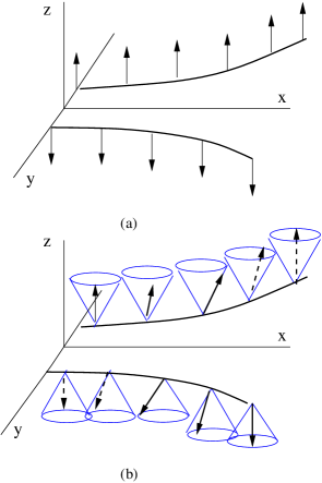
FIG. 1.: Comparison of the usual Stern-Gerlach beam splitting and the topological Stern-Gerlach splitting. When the Zeeman fields are applied along the $z$-direction as shown in Fig.(a), in the conventional Stern-Gerlach splitting ${\bf S}_{z}$ is a good quantum number and no spin rotation occurs; the Zeeman field gradient drives spin-up and spin-down particles apart along the y-direction. However TSGS is always accompanied by spin rotation as shown in Fig.(b). Spins are represented by short arrows in this Figure and other figures.

FIG. 2.: Plus and minus Fermi seas for the toy Hamiltonian in Eq.101, the Rashba Hamiltonian and Dresselhaus Hamiltonian. Fig.(a),(b) are for the toy Hamiltonian. In the plus Fermi sea each spin points at the direction of its momentum (shown in Fig. (a)); in the minus Fermi sea shown in Fig.(b), the spin of an electron points at the opposite direction of its momentum. In Fig. (c) and (d), we show the corresponding Fermi seas for the 2D Rashba Hamiltonian. In $k_{x}-k_{y}$ plane, electron spins in the plus fermi seas form a meron with a half skyrmion charge when a Zeeman field is applied along the $z$-axis. At large ${\bf k}$ limit in the plus Fermi seas, spins point at ${\bf e}\times{\bf\Omega}({\bf k})$ direction while in the minus Fermi seas spins point at $-{\bf e}\times{\bf\Omega}({\bf k})$; they both represent vortices with one unit positive vorticity. Here ${\bf\Omega}({\bf k})$ is a unit vector along ${\bf k}$. At the center of fermi seas, spins are along the $\pm z$ directions (not shown here). In Fig.(e) and (f), we show spin rotation in fermi seas of the Dresselhaus model; electron spins in the plus fermi seas form a meron with a half negative skyrmion charge. At large momentum, electron spins in both fermi seas form vortices with one unit negative vorticity.

FIG. 3.: Topological field $T^{K}$ as a function of $\rho_{\bf k}$ in the 2D Rashba model (schematic). $\lambda_{s}$ which defines the size of meron is chosen to be smaller than the fermi momentum $k_{F}$

FIG. 4.: Responses of Fermi seas and individual electrons to external pumping fields applied along the $x$-direction. Fig.(a) is for polarized electrons in the presence of orbital magnetic fields directing along the $z$-direction; spin-up and spin-down Fermi seas experience identical displacement ${\bf d}$ along the longitudinal direction $x$ and transverse direction $y$ which are shown in two upper left insets of Fermi seas. Fig. (b) is for electrons with spin rotation in the $X$-space; in this case spin-up and spin-down Fermi seas have opposite displacement ${\bf d}$ along the transverse direction $y$ as shown in two insets for two Fermi seas. In Fig.(c) we illustrate differences in electrons’ responses in the plus and minus Fermi seas. We want to emphasize that Fermi seas don’t have collective displacement along a transverse direction $y$ or ${\bf d}_{y}=0$. In insets we show the external-field-induced drift or group velocity of individual electrons ${\bf v}_{y}$ in different regions of fermi seas. The transverse drift of an electron in the upper part of a Fermi sea with momentum ${\bf k}$ is in an opposite direction of the drift of the electron with momentum $-{\bf k}$ in the lower part, which results in self-twists of Fermi seas. In upper(lower) insets, we show the drift of electrons in the north (south) poles of plus and minus fermi seas respectively; the big arrows across Fermi seas indicate the direction of two distinct twists of plus and minus Fermi seas. In Fig.(d), we illustrate responses of the plus and minus fermi seas in the 2D Rashba model; in this case, again two fermi seas have zero displacement in the transverse y-directions (${\bf d}_{y}=0$). However, the spin-plus and spin-minus electrons in two fermi seas acquire a field-induced dispersive group velocities in the opposite $y$-direction as shown in two insets in Fig.(d); the field-induced transveral group velocity decreases rapidly as the momentum increases. See section VII for detailed discussions.

REFERENCES

• [1] R.B.Laughlin, Phys.Rev.B 23, 5632(1981).
• [2] D. J. Thouless, Phys.Rev.B 27, 6083(1983).
• [3] Q. Niu and D. Thouless, J. Phys. A 17, 2453(1984); Q. Niu, D.J. Thouless, and Y.S.Wu, Phys.Rev.B 31, 3372(1985).
• [4] M. Berry, Pro. R. Soc. Lond. A392, 45(1984).
• [5] B. Simon, Phys. Rev. Lett. 51, 2167(1983).
• [6] D. J. Thouless, M. Kohmoto, P. Nightingale, and M. Den Nijs, Phys. Rev. Lett. 49,405(1982).
• [7] J.W. Ye, Y. B. Kim, A.J. Millis, B.I.Shraiman, P. Majumdar, and Z. Tesanovic, Phys. Rev. Lett. 83, 3737(1999); Y. B. Kim, P. Majumdar, A.J.Millis, and B.I.Shraiman, cond-mat/9803350.
• [8] P. Matl, N. P. Ong, Y. F. Yan, Y. Q. Li, D. Studebaker,T. Baum, and G. Doubinina, Phys. Rev. B57,10248(1998).
• [9] G. Sundaram and Q. Niu, Phys. Rev. B 59, R12755(1999).
• [10] T.Jungwirth, Q. Niu and A. H. MacDonald, Phys. Rev. Lett. 88, 207208(2002).
• [11] R. Karplus and J. M . Luttinger, Phys. Rev. 95, 1154 (1954).
• [12] J. Sinova, D. Culcer, Q. Niu, N. A. Sinitsyn, T. Jungwirth, and A. H. MacDonald, cond-mat/0307663; D. Culcer, J. Sinova, N. Sinitsyn, T. Jungwirth, A. H. MacDonald, and Q. Niu, cond-mat/0309475; N. Sinitsyn, E. M. Hankiewicz, W. Teizer, and J. Sinova, cond-mat/0310315.
• [13] M. Onoda and N. Nagaosa, J. Phys. Soc. Jpn.71,19(2002); G. Tatara and H. Kawamura, J. Phys. Soc. Jpn. 71, 2613(2002).
• [14] S.Murakami, N. Nagaosa, and S. C. Zhang, Science 301,1348(2003).
• [15] S.Murakami, N. Nagaosa, and S. C. Zhang, cond-mat/0310005.
• [16] B. A. Bernevig, J. P. Hu, E. Mukamel, and S. C. Zhang, Cond-mat/0311024.
• [17] F.Zhou, B. Spivak, and B. Altshuler, Phys. Rev. Lett. 82, 608(1999).
• [18] F.Zhou, cond-mat/0202321; see also F. Zhou, Phys. Rev. B 65, 220514(2002).
• [19] J. M. Luttinger, Phys. Rev. Rev. 102, 1030(1956).
• [20] G. Dresselhaus, Phys. Rev. 100,580(1955).
• [21] R. I. Rashba, Soviet Physics Solid State 2, 1109(1960).
• [22] E.I. Rashba and V. I. Sheka, Sov. Phys. Solid State 3, 1257(1961).
• [23] Y. A. Bychkov and E. I. Rashba, Sov. Phys. JETP Lett. 39,78 (1984).
• [24] E. I. Rashba, cond-mat/03090441.
• [25] The notion of meron was first introduced in D. J. Gross, Nucl. Phys. B 132, 439(1978). I want to thank Ian Affleck for bringing this reference to my attention.
• [26] The mass generation by merons in spin chains was discussed in I. Affleck, Phys. Rev. Lett.56, 408(1986). See also related discussions on spin gap in F. D. Haldane, Phys. Rev. Lett. 50, 1153 (1983).
• [27] B. Spivak, F. Zhou, and M. T. Beal Monod, Phys. Rev. B51, 13226(1995).
• [28] This is a stringent sufficient condition. However if the main contribution to currents is from electrons with momentum $k_{F}$ away from the ${\bf k}=0$ point, the condition can be relaxed and is always satisfied.
• [29] When the contributions to currents are mainly from the Fermi surface as in the toy model discussed in section VI.A, the adiabaticity condition can be easily satisfied because of the finite splitting between two spin bands due to spin-orbit coupling. However, in the 2D models studied here contributions might actually come from states in the vicinity of ${\bf k}=0$; to establish the adiabaticity condition it is essential to introduce a finite Zeeman field so to split the degeneracy at ${\bf k}=0$ as shown in Eq.152. Then the Born approximation is still applicable when the impurity potentials are weak compared with the finite Zeeman field splitting.
• [30] P. Brouwer, Phys. Rev. B58, 10135(1998).
• [31] F.Zhou, Int. Jour. Mod. Phys.B, 117(2001).
• [32] M. Switkes, C.Marcus, K. Campman, and A. Gossard, Science 283, 1907(1999).
• [33] T. A. Shutenko, I. Aleiner, and B. I. Altshuler, Phys. Rev.B 61, 10366(2000).
• [34] L. S. Levitov, Cond-mat/0103617.
• [35] P. Sharma, and C. Chamon, Phys. Rev. Lett. 87,096401(2001).
• [36] R. Mucciolo, C. Chamon, and C. Marcus, Phys. Rev. Lett. 89, 146802(2002).
• [37] J. Wu, B. Wang, and J. Wang, Phys. Rev.B66, 205327 (2002).
• [38] W. Zheng, J.L. Wu, B. G. Wang, J. Wang, Q. F. Sun, and H. Guo, Phys. Rev. B68, 113306(2003).
• [39] S. K. Watson. R. M. Potok, C. Marcus, and V. Umansky, cond-mat/0302492.
• [40] P. Sharma and P. Brouwer, Phys. Rev. Lett.91, 166801(2003).
• [41] J. Schliemann and D. Loss, cond-mat/0310108.
Refer to caption