Spin models with random anisotropy and reflection symmetry

Abstract

We study the critical behavior of a general class of cubic-symmetric spin systems in which disorder preserves the reflection symmetry $s_{a}\to-s_{a}$, $s_{b}\to s_{b}$ for $b\not=a$. This includes spin models in the presence of random cubic-symmetric anisotropy with probability distribution vanishing outside the lattice axes. Using nonperturbative arguments we show the existence of a stable fixed point corresponding to the random-exchange Ising universality class. The field-theoretical renormalization-group flow is investigated in the framework of a fixed-dimension expansion in powers of appropriate quartic couplings, computing the corresponding $\beta$-functions to five loops. This analysis shows that the random Ising fixed point is the only stable fixed point that is accessible from the relevant parameter region. Therefore, if the system undergoes a continuous transition, it belongs to the random-exchange Ising universality class. The approach to the asymptotic critical behavior is controlled by scaling corrections with exponent $\Delta=-\alpha_{r}$, where $\alpha_{r}\simeq-0.05$ is the specific-heat exponent of the random-exchange Ising model.

I Introduction and summary

The critical behavior of magnetic systems in the presence of quenched disorder has been the subject of extensive theoretical and experimental study. An important class of systems is formed by amorphous alloys of rare earths with aspherical electron distribution and transition metals, for instance TbFe₂ and YFe₂. These systems are modeled [1, 2] by the Heisenberg model with random uniaxial single-site anisotropy, or, in short, by the random-anisotropy model (RAM)

$${\cal H}_{\rm RAM}=-J\sum_{\langle xy\rangle}\vec{s}_{x}\cdot\vec{s}_{y}-D_{0}\sum_{x}(\vec{u}_{x}\cdot\vec{s}_{x})^{2},$$ (1)

where $\vec{s}_{x}$ is an $M$-component spin variable, $\vec{u}_{x}$ is a unit vector describing the local (spatially uncorrelated) random anisotropy, and $D_{0}$ the anisotropy strength. In amorphous alloys the distribution of $\vec{u}_{x}$ is usually taken to be isotropic, since in the absence of crystalline order there is no preferred direction. On the other hand, in polycrystalline materials, for instance in the Laves-phase intermetallic (Dy_xY_1-x)Al₂ compounds studied in Refs. [3, 4], the distribution of $\vec{u}_{x}$ is expected to have only the lattice symmetry.

The critical behavior, and in particular the nature of the low-temperature phase, of a generic system with random anisotropy depends on the probability distribution of the random vector $\vec{u}_{x}$. In the isotropic case, i.e. when the probability distribution is uniformly weighted over the $(M-1)$-dimensional sphere, the Imry-Ma argument [5, 6] forbids the appearance of a low-temperature phase with nonvanishing magnetization for $d<4$. This still allows the presence of a finite-temperature transition with a low-temperature phase in which correlation functions decay algebraically, as it happens in the two-dimensional XY model. Such a behavior has been predicted for the RAM with isotropic distribution in Ref. [7] and it has been recently supported by a $4-\epsilon$ study [8, 9] using the functional renormalization group (RG) [10]. On the other hand, standard field-theoretical perturbative approaches do not find any evidence for a critical behavior with long-range correlations [11, 12, 13, 14]. While experiments have not yet found evidence of low-temperature quasi long-range order, numerical simulations seem to confirm the picture of Refs. [7, 8, 9], but are still contradictory as far as universality and behavior in the strong-anisotropy regime are concerned [15, 16]. For these reasons, the critical behavior of the RAM can still be considered as an open problem.

The above arguments do not apply to spin models with the discrete anisotropic distribution introduced in Ref. [11], in which the vector $\vec{u}_{x}$ points only along one of the $M$ lattice axes, i.e. it has the probability distribution

$$P_{c}(\vec{u})=\frac{1}{2M}\sum_{a=1}^{M}[\delta^{(M)}(\vec{u}-\hat{x}_{a})+\delta^{(M)}(\vec{u}+\hat{x}_{a})],$$ (2)

where $\hat{x}_{a}$ is a unit vector which points in the positive $a$ direction. This model, which we shall call random cubic anisotropic model (RCAM), should have a standard order-disorder transition: The random discrete cubic anisotropy should stabilize a low-temperature phase with long-range ferromagnetic order. On the basis of two-loop calculations in field-theoretical frameworks, it has been argued [17, 18] that the transition belongs to the universality class of the random-exchange Ising model (REIM) for any number $M$ of components.

In this paper we study the critical properties of the three-dimensional RCAM. We consider the field-theoretical approach based on the Landau-Ginzburg-Wilson $\varphi^{4}$ Hamiltonian [11]

$${\cal H}_{\rm LGW}=\int d^{d}x\left\{\sum_{i,a}\frac{1}{2}\left[(\partial_{\mu}\phi_{ai})^{2}+r\phi_{ai}^{2}\right]+\frac{1}{4!}\sum_{ijab}(u_{0}+v_{0}\delta_{ij}+w_{0}\delta_{ab}+y_{0}\delta_{ij}\delta_{ab})\phi_{ai}^{2}\phi_{bj}^{2}\right\},$$ (3)

where $a,b=1,\ldots M$ and $i,j=1,\ldots N$. In the limit $N\rightarrow 0$ the Hamiltonian (3) is expected to describe the critical behavior of the RCAM for $M$-component spins. Using nonperturbative arguments, we show that the field theory with Hamiltonian (3) has two stable fixed points (FP’s). One of them belongs to the REIM universality class while the other corresponds to the O($N$) model in the limit $N\rightarrow 0$, the so-called self-avoiding-walk universality class. Then, we investigate the RG flow for the model with Hamiltonian (3) in the framework of a fixed-dimension expansion in powers of appropriate zero-momentum quartic couplings. We compute the corresponding Callan-Symanzik $\beta$-functions to five loops. Their analysis shows that the only accessible stable FP from the region of parameters relevant for the RCAM is the REIM FP. This implies that the critical behavior of the RCAM (when the parameters allow a continuous transition) belongs to the REIM universality class, whose critical exponents are [19] $\nu_{r}=0.683(3)$, $\alpha_{r}=-0.049(9)$, $\eta_{r}=0.035(2)$, etc. The approach to the REIM scaling behavior is characterized by very slowly decaying scaling corrections proportional to $t^{\Delta}$ with $\Delta=-\alpha_{r}\approx 0.05$, which is much smaller than the scaling-correction exponent of the REIM, which is [20, 21] $\Delta_{r}\approx 0.25$. Our results fully confirm and put on a firmer ground the conclusions of Refs. [17, 18] based on two-loop perturbative calculations.

It is important to note that our results are specific of distributions that vanish everywhere outside the lattice axes, such as the one given in Eq. (2). Indeed, generic cubic-symmetric distributions $P(\vec{u})$, and in particular the isotropic one, give rise to an additional quartic term that should be added to the effective Hamiltonian (3), i.e.

$$z_{0}\;\sum_{ijab}\phi_{ai}\phi_{bi}\phi_{aj}\phi_{bj}\;.$$ (4)

The REIM FP is unstable with respect to this perturbation. We shall evaluate the corresponding crossover exponent, finding $\phi_{z}=0.79(4)$. Therefore, even small differences from the discrete distribution $P_{c}(\vec{u})$ cause a crossover to a different critical behavior. Nonetheless, when $P_{c}(\vec{u})$ turns out to be a good effective approximation—this might be the case in some crystalline cubic-symmetric random-anisotropy systems—REIM critical behavior may be observed in a preasymptotic region.

The general Landau-Ginzburg-Wilson Hamiltonian (3) can also be recovered by considering systems with cubic anisotropy such that disorder preserves the symmetry $s_{x,a}\to-s_{x,a}$, $s_{x,b}\to s_{x,b}$, $b\not=a$. A general Hamiltonian with this property is given by

$${\cal H}=-J\sum_{\langle xy\rangle}\vec{s}_{x}\cdot\vec{s}_{y}-K\sum_{x}\sum_{a}{s}_{x,a}^{4}-D_{0}\sum_{x}\sum_{a}{q}_{x,a}{s}_{x,a}^{2},$$ (5)

where $s_{x}^{\,2}=1$ and $\vec{q}_{x}$ is a random vector with a probability distribution that is invariant under the interchange $q_{a}\leftrightarrow q_{b}$. The exact reflection symmetry at fixed disorder—this symmetry is not present in generic models of type (1)—is the key property that allows the RCAM and the more general class of models (5) to have a standard order-disorder transition with a low-temperature magnetized phase.

The paper is organized as follows. In Sec. II we apply the replica method to the $\varphi^{4}$ theory corresponding to models (1) and (5), determining the corresponding $\phi^{4}$ Hamiltonians that are the basis of the field-theoretical approach. In Sec. III we discuss some general properties of the theory (3). In particular, we discuss the crossover behavior when randomness is weak, and we prove that the REIM FP is stable by evaluating its stability eigenvalues. In Sec. IV we investigate the RG flow by computing and analyzing the five-loop fixed-dimension expansion of the $\beta$-functions associated with the zero-momentum quartic couplings. In App. A we report a six-loop calculation of the RG dimensions of the bilinear operators in cubic-symmetric models that are used in the discussion of the stability of the FP’s. App. B reports the proof of some identities used in the paper.

II Effective $\mathbf{\Phi}^{4}$ Hamiltonians

The mapping of the RAM Hamiltonian (1) to an effective translationally-invariant $\phi^{4}$ Hamiltonian was originally discussed in Ref. [11]. In order to replace fixed-length spins with uncostrained variables, one performs a Hubbard-Stratonovich transformation. Then, for the purpose of studying the critical behavior one considers the continuum limit of the resulting Hamiltonian and truncates its potential to fourth order. This leads to an effective continuum $\varphi^{4}$ Hamiltonian for an $M$-component real field $\varphi_{a}$

$${\cal H}_{\varphi^{4}}=\int d^{d}x\left[\frac{1}{2}(\partial_{\mu}\vec{\varphi})^{2}+\frac{1}{2}r\vec{\varphi}^{\,2}-D(\vec{u}\cdot\vec{\varphi})^{2}+\frac{1}{4!}v_{0}(\vec{\varphi}^{\,2})^{2}\right],$$ (6)

where $\vec{u}_{x}$ is an external spatially uncorrelated vector field with parity-symmetric distribution $P(\vec{u})$ and $D$ is proportional to $D_{0}$. We relax here the condition $\vec{u}^{\,2}_{x}=1$ and require only that $\langle\vec{u}^{\,2}_{x}\rangle=1$, thereby fixing the normalization of $D$. Using the standard replica trick it is possible to replace the quenched average with an annealed one. The system is replaced by $N$ noninteracting copies with annealed disorder. Then, by integrating over disorder, one obtains the following effective Hamiltonian

$$H_{\rm repl}=\int d^{d}x\left[\sum_{i,a}\frac{1}{2}(\partial_{\mu}\phi_{ai})^{2}+\frac{1}{2}r\sum_{ia}\phi_{ai}^{2}+\frac{1}{4!}v_{0}\sum_{ijab}\delta_{ij}\phi_{ai}^{2}\phi_{bj}^{2}+R(\phi)\right]\,,$$ (7)

where $a,b=1,\ldots M$, $i,j=1,\ldots N$, and

$$R(\phi)=-{\rm ln}\int d^{N}u\,P(\vec{u})\,{\rm exp}\left(D\sum_{iab}u_{a}u_{b}\phi_{ai}\phi_{bi}\right).$$ (8)

In the limit $N\rightarrow 0$ the Hamiltonian (7) is equivalent to the Hamiltonian (6) with quenched disorder. The expansion in powers of the field $\phi$ can be expressed in terms of the moments of the distribution $P(\vec{u})$,

$$M_{a_{1}a_{2}...a_{k}}\equiv\int d^{N}u\,P(\vec{u})\,u_{a_{1}}u_{a_{2}}...u_{a_{k}}\;.$$ (9)

One obtains

$$H_{\rm repl}=\int d^{d}x\left[\frac{1}{2}\sum_{ia}(\partial_{\mu}\phi_{a,i})^{2}+\frac{1}{2}r\sum_{ia}\phi_{a,i}^{2}+\frac{1}{4!}v_{0}\sum_{iab}\phi_{ai}^{2}\phi_{bi}^{2}\right.$$ (10)

$$\left.-D\sum_{iab}M_{ab}\phi_{ai}\phi_{bi}+\frac{1}{2}D^{2}(\sum_{iab}M_{ab}\phi_{ai}\phi_{bi})^{2}-\frac{1}{2}D^{2}\sum_{ijabcd}M_{abcd}\phi_{ai}\phi_{bi}\phi_{cj}\phi_{dj}+O(\phi^{6})\right]\;.$$ (11)

Let us consider the case in which all field components become critical at $T_{c}$. This is achieved if the distribution $P(\vec{u})$ is such that

$$M_{ab}={1\over M}\delta_{ab}.$$ (12)

This condition is satisfied if $P(u)$ is cubic symmetric. Under this further assumption, the fourth moment $M_{abcd}$ can be written as

$$M_{abcd}=A\left(\delta_{ab}\delta_{cd}+\delta_{ac}\delta_{bd}+\delta_{ad}\delta_{bc}\right)+B\delta_{abcd}\;,$$ (13)

where $A$ and $B$ are parameters depending on the distribution that satisfy the Cauchy inequalities $A(M+2)+B\geq 1/M$ and $3A+B\geq 1/M^{2}$. It follows that

$$H_{\rm repl}=\int d^{d}x\left[\vphantom{{D^{2}\over 2M^{2}}}\frac{1}{2}\sum_{ia}(\partial_{\mu}\phi_{ai})^{2}+\frac{1}{2}(r-D/M)\sum_{ia}\phi_{ai}^{2}+\frac{1}{4!}v_{0}\sum_{iab}\phi_{ai}^{2}\phi_{bi}^{2}+\right.$$ (14)

$$\left.+{D^{2}\over 2M^{2}}(1-M^{2}A)(\sum_{ia}\phi_{ai}^{2})^{2}-AD^{2}\sum_{ijab}\phi_{ai}\phi_{bi}\phi_{aj}\phi_{bj}-{BD^{2}\over 2}\sum_{ija}\phi_{ai}^{2}\phi_{aj}^{2}+O(\phi^{6})\right].$$ (15)

In conclusion, for generic cubic-symmetric distributions $P(\vec{u})$ the Hamiltonian that should describe the critical behavior of the corresponding RAM is

$${\cal H}= \int d^{d}x\left\{\frac{1}{2}\sum_{ia}(\partial_{\mu}\phi_{ai})^{2}+\frac{1}{2}r\sum_{ia}\phi_{ai}^{2}+\right.$$ (17)

$$\left.+\frac{1}{4!}\sum_{ijab}\Bigl{[}(u_{0}+v_{0}\delta_{ij}+w_{0}\delta_{ab}+y_{0}\delta_{ij}\delta_{ab})\phi_{ai}^{2}\phi_{bj}^{2}+z_{0}\phi_{ai}\phi_{bi}\phi_{aj}\phi_{bj}\right\},$$

where the term proportional to $y_{0}$ has been added because it is generated by RG iterations whenever $w_{0}\not=0$. It should be noticed that such a term arises naturally if one considers that, if the system is only cubic symmetric, quartic single-ion terms must be included. In this case it is natural to consider

$${\cal H}=-J\sum_{\langle xy\rangle}\vec{s}_{x}\cdot\vec{s}_{y}-D_{0}\sum_{x}(\vec{u}_{x}\cdot\vec{s}_{x})^{2}+K\sum_{x}\sum_{a}s_{x,a}^{4},$$ (18)

and the corresponding $\varphi^{4}$ Hamiltonian

$${\cal H}=\int d^{d}x\left[\frac{1}{2}(\partial_{\mu}\vec{\varphi})^{2}+\frac{1}{2}r\vec{\varphi}^{\,2}-D(\vec{u}\cdot\vec{\varphi})^{2}+\frac{1}{4!}v_{0}(\vec{\varphi}^{\,2})^{2}+\frac{1}{4!}y_{0}\sum_{a}\varphi_{a}^{4}\right].$$ (19)

The Hamiltonian (17) was originally introduced in Ref. [12] to describe magnetic systems with single-ion anisotropy and nonmagnetic impurities.

There are two interesting particular cases. First, one may consider an $O(M)$-invariant pure system coupled to an isotropic distribution $P(u)$. In this case $K=0$ in Eq. (18)—therefore, $y_{0}=0$—and $B=0$ in Eq. (13), so that $w_{0}=0$. These conditions are preserved under renormalization by the presence of the $O(M)$ invariance. Note that this is not the case if $K\not=0$, i.e. if $y_{0}\not=0$. Distributions such that $B=0$ (these distributions are not necessarily isotropic) give apparently $w_{0}=0$; however, such a condition is not preserved under renormalization if $z_{0}\not=0$.

A second interesting case corresponds to distributions $P(u)$ such that $A=0$ in Eq. (13). It is easy to show that distributions $P(u)$ with this property are simple generalizations of the distribution (2). Explicitly, they have the form

$$P(u)={1\over M}\sum_{a}f(u_{a})\prod_{b\not=a}\delta(u_{b}),$$ (20)

where $f(x)$ is a normalized probability distribution with unit variance. If $A=0$, Eq. (15) implies $z_{0}=0$. Such a condition is stable under renormalization. Indeed, the transformation $\phi_{ai}\to-\phi_{ai}$ for fixed $a$ and $i$ is a symmetry of the Hamiltonian with $z_{0}=0$, but not of the term proportional to $z_{0}$. This symmetry is due to the fact that, for distributions of type (20), we can write $(\vec{s}\cdot\vec{u})^{2}=\sum_{a}u^{2}_{a}s_{a}^{2}$, which is symmetric under the transformations $s_{a}\to-s_{a}$ at fixed $u$. In other words, the theory with $z_{0}=0$ describes models in which the reflection symmetry of the spins is also preserved at fixed disorder.

In the case of discrete cubic-symmetric distributions of type (20), we have

$$u_{0}={12D^{2}\over M^{2}},\qquad w_{0}=-{12BD^{2}}\;.$$ (21)

Apparently, these conditions imply

$$u_{0}>0,\qquad w_{0}<0,\qquad Mu_{0}+w_{0}\leq 0,$$ (22)

where the last condition follows from the bound $B\geq 1/M$. The equality $Mu_{0}+w_{0}=0$ is obtained by using distribution (2). Relations (21) and (22) should be considered as indicative, since the mapping between the $\varphi^{4}$ Hamiltonian (19) and the general Hamiltonian (17) gives also rise to higher-order terms.

It is also interesting to consider the effective continuum Hamiltonian corresponding to Eq. (5). In this case we obtain

$${\cal H}_{\varphi^{4}}=\int d^{d}x\left[\frac{1}{2}(\partial_{\mu}\vec{\varphi})^{2}+\frac{1}{2}r\vec{\varphi}^{\,2}-D\sum_{a}{q}_{a}\varphi^{2}_{a}+\frac{1}{4!}v_{0}(\vec{\varphi}^{\,2})^{2}+\frac{1}{4!}y_{0}\sum_{a}\varphi_{a}^{4}\right].$$ (23)

If $P(q)$ is invariant under the interchanges $q_{a}\leftrightarrow q_{b}$, we can write for the first moments $M_{a}=a$ and $M_{ab}=b+c\delta_{ab}$. A simple calculation gives again the general Hamiltonian (17) with $z_{0}=0$ and

$$u_{0}={D^{2}\over 2}(a^{2}-b),\qquad w_{0}=-{cD^{2}\over 2}.$$ (24)

Since $b+c\geq a^{2}$, we obtain

$$u_{0}+w_{0}\leq 0.$$ (25)

Equality is obtained for $P(q)=\prod_{a}\delta(q_{a}-1)$ (in this case however $w_{0}=0$). Finally, note that if $c=0$ then we have $w_{0}=0$. Such a condition is stable under renormalization, and thus this class of models is expected to have a different critical behavior. It corresponds to the one of the randomly dilute cubic models discussed in Ref. [22]. Distributions with this property are however quite peculiar. They have the general form

$$P(q)=f(q_{1})\prod_{a=2}^{M}\delta(q_{1}-q_{a}).$$ (26)

The stability region of the quartic potential in the $\varphi^{4}$ Hamiltonian (3) is given by the conditions

$$Nu_{0}+v_{0}+Nw_{0}+y_{0}>0,$$ (27)

$$NMu_{0}+Mv_{0}+Nw_{0}+y_{0}>0,$$ (28)

$$u_{0}+v_{0}+w_{0}+y_{0}>0,$$ (29)

$$Mu_{0}+Mv_{0}+w_{0}+y_{0}>0.$$ (30)

However, as discussed in Ref. [12], in the zero-replica limit $N\rightarrow 0$, the only relevant stability conditions are those obtained by using replica-symmetric configurations. Therefore, for the RCAM one should only consider Eqs. (27) and (28) with $N=0$, i.e.

$$v_{0}+y_{0}>0 \qquad\hbox{\rm if }v_{0}>0,$$ (31)

$$Mv_{0}+y_{0}>0 \qquad\hbox{\rm if }v_{0}<0.$$ (32)

Equivalently, the relevant stability conditions can be obtained by considering the Hamiltonians (19) and/or (23).

III General renormalization-group properties

A Fixed points of the theory

The properties of the RG flow are essentially determined by its FP’s. Most of them can be identified by considering the theories obtained when some of the quartic parameters vanish. For example, we can easily recognize:

(a) the O($M\times N$) theory for $v_{0}=w_{0}=y_{0}=0$;

(b) $N$ decoupled O($M$) theories for $u_{0}=w_{0}=y_{0}=0$;

(c) $M$ decoupled O($N$) theories for $u_{0}=v_{0}=y_{0}=0$;

(d) $M\times N$ decoupled Ising theories for $u_{0}=v_{0}=w_{0}=0$;

(e) the $MN$ model (see, e.g., Refs. [23, 24]) for $w_{0}=y_{0}=0$;

(f) the $NM$ model for $v_{0}=y_{0}=0$;

(h) $N$ decoupled $M$-component cubic models for $u_{0}=w_{0}=0$;

(i) $M$ decoupled $N$-component cubic models for $u_{0}=v_{0}=0$;

(j) $M\times N$-component cubic model for $v_{0}=w_{0}=0$;

(k) the randomly dilute $M$-component cubic model (see Ref. [22]) for $w_{0}=0$ and $N=0$;

(l) the tetragonal model [23, 25] for $M=2$ and $w_{0}=0$.

The FP’s of these theories are also FP’s of the enlarged model (3). Of course, there may also be FP’s that are not related to the above particular cases. Their presence can be investigated by low-order $\epsilon$ expansion calculations. First-order $\epsilon$-expansion calculations [11] show the presence of 14 FP’s for $M\neq 2$ and of 13 FP’s for $M=2$. As in the REIM case, at two-loop order other $O(\sqrt{\epsilon})$ FP’s appear [12]: 4 FP’s for $M\neq 2$ and 6 FP’s for $M=2$ [17]. The two-loop $\epsilon$-expansion results are summarized in Refs. [17, 18]. In Table I we report the leading $\epsilon$-expansion terms for the location of the FP’s (in the minimal-subtraction renormalization scheme) and the corresponding stability eigenvalues. The only stable FP’s are the O(0) and the REIM FP’s, which are already present in models (a) and (i), respectively. These results have also been supported by two-loop fixed-dimension calculations [17]. In order to understand the relevance of the various FP’s for the RCAM, we need to check which one is accessible from the region of the quartic parameters relevant for the three-dimensional RCAM. This issue will be investigated in Sec. IV computing and analyzing five-loop series in the framework of the fixed-dimension expansion.

TABLE I.: Fixed points of the Hamiltonian (3) near four dimensions. We report the leading nontrivial contribution of the expansion in powers of $\epsilon$, taken from Refs. [11, 17]. Here, $K_{d}=(4\pi)^{d}\Gamma(d/2)/2$, $\alpha_{\pm}=(M-4\pm\sqrt{M^{2}+48})/8$, $\beta_{\pm}=-(M+12\pm\sqrt{M^{2}+48})/6$, $A_{\pm\pm}=6\alpha_{\pm}+3\beta_{\pm}+M+6$. The general expressions for the stability eigenvalues of FP’s XI-XIV are rather cumbersome. We only report their numerical value for $M=3$.

		$v^{*}/K_{d}$	$u^{*}/K_{d}$	$w^{*}/K_{d}$	$y^{*}/K_{d}$	Stability eigenvalues
I	Gaussian	0	0	0	0	$\omega_{u}=\omega_{v}=\omega_{w}=\omega_{y}=-\epsilon$
II	O(M)	$\frac{6}{M+8}\epsilon$	0	0	0	$\omega_{v}=\epsilon,\omega_{u}=-\frac{4-M}{M+8}\epsilon,\omega_{w}=-\frac{4+M}{M+8}\epsilon,\omega_{y}=\frac{4-M}{M+8}\epsilon$
III	O(0)	0	$\frac{3}{4}\epsilon$	0	0	$\omega_{u}=\epsilon,\omega_{v}=\omega_{w}=\omega_{y}=\epsilon/2$
IV	O(0)	0	0	$\frac{3}{4}\epsilon$	0	$\omega_{u}=\omega_{v}=-\epsilon/2,\omega_{w}=\epsilon,\omega_{y}=\epsilon/2$
V	Ising	0	0	0	$\frac{2}{3}\epsilon$	$\omega_{u}=\omega_{v}=\omega_{w}=-\epsilon/3,\omega_{y}=\epsilon$
VI		$\frac{3}{2(M-1)}\epsilon$	$\frac{3(M-4)}{8(M-1)}\epsilon$	0	0	$\omega_{1}=\epsilon,\omega_{2}=\omega_{y}=\frac{4-M}{4(M-1)}\epsilon,\omega_{w}=-\frac{4+M}{4(M-1)}\epsilon$
VII		0	$\frac{3}{2}\epsilon$	$-\frac{3}{2}\epsilon$	0	$\omega_{1}=\omega_{v}=\epsilon,\omega_{3}=\omega_{y}=-\epsilon$
VIII	Cubic	$\frac{2}{M}\epsilon$	0	0	$\frac{2(M-4)}{3M}\epsilon$	$\omega_{u}=\omega_{2}=-\frac{4-M}{3M}\epsilon,\omega_{w}=-\frac{4+M}{3M}\epsilon,\omega_{4}=\epsilon$
IX	$M\neq 2$	$\frac{1}{M-2}\epsilon$	$\frac{M-4}{4(M-2)}\epsilon$	0	$\frac{M-4}{3(M-2)}\epsilon$	$\omega_{1}=\epsilon,\omega_{2}=\frac{4-M}{6(M-2)}\epsilon,\omega_{w}=\frac{-(4+M)}{6(M-2)},\omega_{4}=\frac{-(4-M)}{6(M-2)}\epsilon$
X		0	$\frac{1}{2}\epsilon$	$-\frac{1}{2}\epsilon$	$\frac{2}{3}\epsilon$	$\omega_{1}=\epsilon,\omega_{v}=\omega_{3}=\epsilon/3,\omega_{4}=-\epsilon/3$
XI		$\frac{3}{A_{++}}\epsilon$	$\frac{3\alpha_{+}}{A_{++}}\epsilon$	$\frac{3(M+4)}{4A_{++}}\epsilon$	$\frac{3\beta_{+}}{A_{++}}\epsilon$	$\omega_{1}=\epsilon,\omega_{2}=1.33\epsilon,\omega_{3}=\omega_{4}=-1.43\epsilon$ (for $M=3$)
XII		$\frac{3}{A_{+-}}\epsilon$	$\frac{3\alpha_{+}}{A_{+-}}\epsilon$	$\frac{3(M+4)}{4A_{+-}}\epsilon$	$\frac{3\beta_{-}}{A_{+-}}\epsilon$	$\omega_{1}=\epsilon,\omega_{2}=-\omega_{3}=0.371\epsilon,\omega_{4}=-0.344\epsilon$ (for $M=3$)
XIII		$\frac{3}{A_{-+}}\epsilon$	$\frac{3\alpha_{-}}{A_{-+}}\epsilon$	$\frac{3(M+4)}{4A_{-+}}\epsilon$	$\frac{3\beta_{+}}{A_{-+}}\epsilon$	$\omega_{1}=\epsilon,\omega_{2}=-\omega_{3}=0.435,\omega_{4}=-0.403\epsilon$ (for $M=3$)
XIV		$\frac{3}{A_{--}}\epsilon$	$\frac{3\alpha_{-}}{A_{--}}\epsilon$	$\frac{3(M+4)}{4A_{--}}\epsilon$	$\frac{3\beta_{-}}{A_{--}}\epsilon$	$\omega_{1}=\epsilon,\omega_{2}=\omega_{3}=-3.32\epsilon,\omega_{4}=-3.08\epsilon$ (for $M=3$)
XV	REIM	0	0	$\mp\sqrt{\frac{54}{53}}\sqrt{\epsilon}$	$\pm\frac{4}{3}\sqrt{\frac{54}{53}}\sqrt{\epsilon}$	$\omega_{u}=\omega_{v}=\omega_{1}=\pm\sqrt{\frac{24}{53}}\sqrt{\epsilon},\omega_{2}=2\epsilon$
XVI	REIM	0	$\mp\sqrt{\frac{54}{53}}\sqrt{\epsilon}$	0	$\pm\frac{4}{3}\sqrt{\frac{54}{53}}\sqrt{\epsilon}$	$\omega_{w}=\omega_{v}=-\omega_{1}=\mp\sqrt{\frac{24}{53}}\sqrt{\epsilon},\omega_{2}=2\epsilon$
XVII	$M=2$	$\mp 2\sqrt{\frac{54}{53}}\sqrt{\epsilon}$	$\pm\sqrt{\frac{54}{53}}\sqrt{\epsilon}$	0	$\pm\frac{4}{3}\sqrt{\frac{54}{53}}\sqrt{\epsilon}$	$\omega_{w}=\omega_{3}=-\omega_{1}=\mp\sqrt{\frac{24}{53}}\sqrt{\epsilon},\omega_{2}=2\epsilon$

B Crossover behavior close to the pure spin model

The O($M$)-symmetric FP located in the $v$-axis describes the critical properties of the pure spin system in the absence of cubic anisotropy. It is interesting to compute the crossover exponent in the presence of random anisotropy. Setting $t_{p}\equiv(T-T_{p})/T_{p}$, where $T_{p}\equiv T_{c}(D_{0}=0)$ is the critical temperature in the absence of anisotropy, in the limit $t_{p}\to 0$ and $D_{0}\to 0$ the singular part of the free energy can be written as

$${\cal F}=|u_{t}|^{2-\alpha}f(D_{0}^{2}|u_{t}|^{-\phi_{D}}),$$ (33)

where $u_{t}\approx t_{p}+a_{1}D_{0}^{2}+a_{2}t_{p}^{2}+\dots$ is the scaling field associated with temperature, $\alpha$ is the specific-heat exponent in the O($M$) theory, $\phi_{D}$ is the crossover exponent, and $f(x)$ is a scaling function. As a consequence of Eq. (33), for sufficiently small $D_{0}$ the critical-temperature shift is given by

$$\Delta T_{c}(D_{0})\equiv T_{c}(D_{0})-T_{c}(0)\approx aD_{0}^{2/\phi_{D}}+bD_{0}^{2}+cD_{0}^{4}+\ldots$$ (34)

The crossover exponent $\phi_{D}$ is related to the largest positive RG dimension of the perturbations at the O($M$) FP that are present in the Hamiltonian (3), i.e. of the terms proportional to $u_{0}$, $w_{0}$, and $y_{0}$. For $u_{0}=w_{0}=y_{0}=0$, the Hamiltonian (3) describes $N$ decoupled O($M$)-symmetric systems. The RG dimension of the terms proportional to $u_{0}$ and $w_{0}$ can be determined by writing [11]

$$\sum_{abij}(u_{0}+w_{0}\delta_{ab})\phi^{2}_{ai}\phi^{2}_{bj}=M(Mu_{0}+w_{0})\sum_{ij}{\cal E}_{i}{\cal E}_{j}+w_{0}\sum_{ija}{\cal T}_{aai}{\cal T}_{aaj},$$ (35)

where

$${\cal E}_{i} \equiv \frac{1}{M}\sum_{a}\phi_{ai}^{2},$$ (36)

$${\cal T}_{abi} \equiv \phi_{ai}\phi_{bi}-\delta_{ab}{\cal E}_{i}.$$ (37)

The bilinears ${\cal E}_{i}$ and ${\cal T}_{abi}$ are respectively the energies and the quadratic spin-2 operators of the $N$ decoupled models. If $y_{E}=1/\nu$ and $y_{T}$ are the corresponding RG dimensions, the two terms given above have RG dimensions $y_{u}=2y_{E}-3=\alpha/\nu$ and $y_{w}=2y_{T}-3$. The perturbation proportional to $y_{0}$ does not couple the different replicas and therefore its RG dimension $y_{y}$ is simply the RG dimension of the cubic perturbation, which is related to the RG dimension of the spin-4 perturbation of the $O(M)$ FP [26, 27]. Therefore, the $O(M)$ FP is perturbed by three terms of RG dimensions $y_{u}$, $y_{w}$, and $y_{y}$, which can be determined using known results for the RG dimensions of generic operators in an O($M$) theory, see, e.g., Refs. [28, 25] for reviews of results. Since $\alpha$ is negative for $M\geq 2$, we have $y_{u}<0$ and therefore the corresponding term is always irrelevant. The exponent $y_{T}$ has been obtained by using field-theoretical [26] and Monte Carlo methods [29]: field-theoretical analyses give $y_{T}=1.766(6)$ for $M=2$ and $y_{T}=1.790(3)$ for $M=3$, while Monte Carlo simulations give $y_{T}=1.756(2)$ for $M=2$ and $y_{T}=1.787(2)$ for $M=3$. Correspondingly, we find $y_{w}=0.532(12)$ and $y_{w}=0.511(6)$ for $M=2$, and $y_{w}=0.580(6)$ and $y_{w}=0.573(3)$ for $M=3$. Therefore, the perturbation proportional to $w_{0}$ is always relevant. Finally, using the results of Refs.[26, 27] for the spin-4 perturbations at the O($M$) FP, we have $y_{y}=-0.103(8)$ for $M=2$ and $y_{y}=0.013(6)$ for $M=3$. This implies that the $y$-term is irrelevant for $M=2$, but relevant for $M=3$. In conclusion, for both $M=2$ and $M=3$, the most relevant quartic perturbation is given by the $w$-term, which determines the crossover from the pure critical behavior in the limit of small anisotropy strength. Therefore, $\phi_{D}=y_{w}\nu=0.357(3)$ for $M=2$ and $\phi_{D}=y_{w}\nu=0.412(3)$ for $M=3$. In the crossover limit in which $D_{0}^{2}|u_{t}|^{-\phi_{D}}$ is held fixed, the operators with RG dimensions $y_{u}$ and $y_{y}$ give rise to scaling corrections. In particular, there are corrections proportional to $t^{\Delta_{y}}$, with $\Delta_{y}\equiv y_{y}\nu-\phi_{D}$, $\Delta_{y}=0.426(6)$ for $M=2$ and $\Delta_{y}=0.403(5)$ for $M=3$, which are more important than the usual $O(M)$-invariant corrections, which vanish as $t^{\Delta}$, with [25] $\Delta\approx 0.54$ for $M=2$ and $\Delta\approx 0.56$ for $M=3$.

It is worth mentioning that the scaling behavior (33) with the same crossover exponent $\phi_{D}$ also holds for a RAM with generic distribution $P(\vec{u})$, and in particular for the isotropic case. Indeed, the additional term proportional to $z_{0}$ appearing in the Hamiltonian (17) has the same RG dimension of the $w$-term at the O($M$) FP. This can be inferred by rewriting

$$\sum_{abij}\phi_{ai}\phi_{bi}\phi_{aj}\phi_{bj}=\sum_{abij}{\cal T}_{abi}{\cal T}_{abj}+M\sum_{ij}{\cal E}_{i}{\cal E}_{j},$$ (38)

where ${\cal T}_{abi}$ and ${\cal E}_{i}$ are defined in Eq. (37). The first term is the most relevant one and therefore, we obtain $y_{z}=2y_{T}-3$ and also $y_{z}=y_{w}$.

Let us note that the relatively small value of $\phi_{D}$ makes the measurement of $\phi_{D}$ from the critical-temperature shift for small random anisotropy rather difficult. Indeed, in Eq. (34) the term $D_{0}^{2/\phi_{D}}$ is suppressed with respect to the first two analytic terms proportional to $D_{0}^{2}$ and $D_{0}^{4}$, since $2/\phi_{D}\approx 4.9$ (resp. $2/\phi_{D}\approx 5.6$) for $M=3$ (resp. $M=2$). This explains the results of Ref. [4] that measured $T_{c}$ in crystalline Laves-phase (Dy_xY_1-x)Al₂ for different values of $x$. Since [30] $D_{0}\to 0$ as $x\to 1$, they were able to measure $\Delta T_{c}(D_{0})$ for $D_{0}\to 0$. The experimental results were fitted assuming $\Delta T_{c}(D_{0})\sim D_{0}^{2/\psi}$, obtaining $\psi=0.80(8)$. This result is in substantial agreement with the theoretical prediction $\Delta T_{c}(D_{0})\sim D_{0}^{2}$, but does not provide information on the crossover exponent $\phi_{D}$.

For $M\geq 3$, pure systems with Hamiltonian (18) do not have a critical behavior in the $O(M)$ universality class, see, e.g., Refs. [23, 27, 22]. If the system has [111] as easy direction, its critical behavior belongs to a different universality class with reduced cubic symmetry, while systems with [100] easy axis are expected to show a first-order transition. In the latter type of systems, randomness may soften the first-order transition. This issue shall be discussed in Sec. IV C. On the other hand, we now show that in cubic systems with [111] easy axis randomness is a relevant perturbation and therefore, for small randomness, these systems show a crossover behavior with positive exponent $\phi_{D}$, cf. Eq. (33). For $u_{0}=w_{0}=0$ the Hamiltonian (3) reduces to the one for $N$ decoupled systems with cubic symmetry. The RG dimensions of the terms proportional to $u_{0}$ and $w_{0}$ at the cubic FP provide the crossover exponent $\phi_{D}$. In order to determine them, we use again Eq. (35). The RG dimension of ${\cal E}_{i}$ is $y_{E}=1/\nu$, where $\nu$ is the correlation-length exponent, while that of ${\cal U}_{ai}\equiv{\cal T}_{aai}$, $y_{U}$, is computed in App. A by resumming its six-loop perturbative expansion. Thus, the RG dimensions of the two terms appearing in the right-hand side of Eq. (35), we denote them by $y_{u}$ and $y_{w}$, are given by $y_{u}=2y_{E}-3={\alpha/\nu}$ and $y_{w}=2y_{U}-3$, respectively. Since $\alpha<0$ at the cubic FP for any $M\geq 3$, the first term is irrelevant. On the other hand, the estimates of $y_{U}$ reported in App. A show that $y_{w}>0$ for any $M\geq 3$. For example $y_{w}=0.549(14)$ for $M=3$, and therefore $\phi_{D}=0.387(14)$.

Note that in a generic cubic-symmetric RAM, one should also consider perturbations proportional to $z_{0}$. We use again Eq. (38). However, in the presence of cubic symmetry ${\cal T}_{abi}$, cf. Eq (37), is not an irreducible tensor. One must consider separately ${\cal U}_{ai}\equiv{\cal T}_{aai}$ and ${\cal T}_{abi}$ with $a\not=b$, that have different RG dimensions $y_{U}$ and $y_{T}$. Therefore, the term proportional to $z_{0}$ is the sum of three terms of RG dimensions $2y_{E}-3=\alpha/\nu$, $2y_{U}-3$, and $2y_{T}-3$. The last one is the largest, so that $y_{z}=2y_{T}-3$. Using the results of App. A for $M=3$, we find $y_{z}=0.600(4)$. The exponent $y_{z}$ is larger than $y_{w}$. Therefore, a generic cubic-symmetric RAM shows a different crossover behavior with crossover exponent $\phi_{D}=y_{z}\nu=0.427(3)$.

C Stable fixed points

The critical behavior in the presence of random anisotropy should be described by the stable FP of the theory (3) which is accessible from the RCAM. The two-loop $\epsilon$-expansion calculations of Ref. [17] summarized in Sec. III A find two stable FP’s. One of them is located in the $u$-axis, and it is associated with the O(0) or self-avoiding-walk universality class. This FP is also stable in three dimensions. Indeed, the terms proportional to $v_{0}$, $w_{0}$, and $y_{0}$ are interactions transforming as the spin-4 representation of the O($M\times N$) group. Therefore, they have the same RG dimension which is given by $y_{v,w,y}=-0.37(5)$, obtained in Ref. [26] from the analysis of six-loop fixed-dimension and five-loop $\epsilon$ series. It was argued in Ref. [17], on the basis of two-loop calculations, that the O(0) FP is not accessible from the parameter region relevant for the RCAM. This will be confirmed by the five-loop analysis of the RG flow presented in Sec. IV.

For $u_{0}=v_{0}=0$ the Hamiltonian (3) corresponds to a cubic-symmetric model and, for $N\to 0$, it is the sum of $M$ independent models that are the field-theoretical analog of the REIM. We will now show that the REIM FP is stable in the theory (3). It is sufficient to show that the terms proportional to $u_{0}$ and $v_{0}$ are irrelevant. For this purpose, we rewrite

$$\sum_{ijab}(u_{0}+v_{0}\delta_{ij})\phi^{2}_{ai}\phi^{2}_{bj}=N(Nu_{0}+v_{0})\sum_{a}{\cal E}_{a}^{2}+v_{0}\sum_{ai}{\cal U}_{ai}^{2},$$ (39)

where ${\cal E}_{a}=\frac{1}{N}\sum_{i}\phi_{ai}^{2}$ and ${\cal U}_{ai}=\phi_{ai}^{2}-{\cal E}_{a}$. For $N\to 0$, ${\cal E}_{i}$ and ${\cal U}_{ai}$ have the same RG dimension (see App. A for the proof), $y_{E}=y_{U}=1/\nu_{r}$, where $\nu_{r}$ is the correlation-length critical exponent of the REIM universality class. Therefore, the RG dimension of the perturbation is given by $y_{uv}=2y_{E}-3=\alpha_{r}/\nu_{r}$, where $\alpha_{r}$ is the REIM specific-heat exponent. Since $\alpha_{r}$ is negative, see the estimates reported in Refs. [25, 31, 19], the REIM FP is stable. Using the recent Monte Carlo results reported in Ref. [19], we finally arrive at the estimate $y_{uv}\approx-0.07$. As we shall see in Sec. IV, the REIM FP turns out to be accessible to the RCAM, and no other stable FP exists in the region relevant for the RCAM. Therefore, the REIM universality class describes the critical properties of the RCAM in the case it undergoes a continuous transition. Estimates of several universal quantities for the REIM universality class can be found in Refs. [25, 31, 19, 32]. Note, however, that the critical exponent controlling the leading scaling corrections differs from the one for the REIM, which is [20, 21] $\Delta_{r}\approx 0.25$. In the RCAM the leading scaling correction is due to the Hamiltonian terms proportional to $u_{0}$ and $v_{0}$. They cause slowly decaying corrections of order $t^{\Delta}$ with

$$\Delta=-\alpha_{r}=0.049(9).$$ (40)

If $P(q)=\prod_{a}P_{a}(q_{a})$, i.e. the probability distributions of the variables $q_{a}$ are independent, the stability of the REIM FP can also be proved by starting directly from Eq. (23). Indeed, such a Hamiltonian corresponds to $M$ random-exchange $\varphi^{4}$ models coupled by the term proportional to $v_{0}$. Such a term has the form $\sum_{ab}{\cal E}_{a}{\cal E}_{b}$, where ${\cal E}_{a}={1\over N}\varphi_{a}^{2}$ is the energy of the REIM. Therefore, this perturbation has RG dimension $2/\nu_{r}-3=\alpha_{r}/\nu_{r}$, which is negative. Thus, the coupling among the models is irrelevant, and thus it does not change the universality class of the system. If $P(q)$ does not factorize, the $M$ $\varphi^{4}$ models are also coupled by disorder. The above-reported analysis shows that also this coupling is irrelevant, its RG dimension being $\alpha_{r}/\nu_{r}<0$.

As discussed in Sec. II, in the case of a generic random cubic-symmetric distribution $P(\vec{u})$, the Hamiltonian (17) also contains the term proportional to $z_{0}$. It is important to note that the REIM FP is unstable with respect to this perturbation, since its RG dimension $y_{z}$ is positive at the REIM FP. The dimension of this perturbation, $y_{z}$, can be computed by rewriting the term proportional to $z_{0}$ as

$$\sum_{abij}\phi_{ai}\phi_{bi}\phi_{aj}\phi_{bj}=\sum_{ab}\sum_{i\not=j}{\cal T}_{aij}{\cal T}_{bij}+\sum_{ab}\sum_{i}{\cal U}_{ai}{\cal U}_{bi}+N\sum_{ab}{\cal E}_{a}{\cal E}_{b},$$ (41)

where ${\cal T}_{aij}\equiv\phi_{ai}\phi_{aj}$ with $i\not=j$. Therefore, this perturbation is the sum of three terms that have RG dimensions $2y_{T}-3$, $2y_{U}-3$, and $2y_{E}-3$. Using the results reported in App. A, one finds that the most relevant term is the first one, so that

$$y_{z}=2y_{T}-3.$$ (42)

Using the estimate $y_{T}=2.08(3)$ reported in App. A, one obtains

$$y_{z}=1.16(6),\quad\phi_{z}\equiv y_{z}\nu=0.79(4),$$ (43)

where $\phi_{z}$ is the corresponding crossover exponent.

D Critical behavior for infinitely strong random anisotropy

In this Section, we wish to investigate the general model (5) in the limit of infinite disorder, showing that, under some mild hypotheses for the probability distribution $P(q)$, one has REIM critical behavior for $M=2$ and $M=3$ and no transition for $M\geq 4$. This analysis further confirms the results of Sec. III C.

We first consider the case $D_{0}\to+\infty$. We suppose that the distribution $P(q)$ is such that there is only one direction $k$ such that $q_{k}=\max_{b}q_{b}$ (or at least that this condition is verified with probability one). This is the case if the distribution is continuous and is also true for the distribution $P(q)$ derived from (2) (note that $q_{a}=u^{2}_{a}$). Because of the assumption on $P(q)$, for $D_{0}\to+\infty$ the spin $\vec{s}$ is constrained to lie along the $k$ direction, i.e. $s_{k}=\pm 1$, $s_{a}=0$ for $a\not=k$. Thus, in this limit we can rewrite the Hamiltonian in the following way. At each site we define $M$ Ising variables $\sigma_{x,a}$ and $M$ disorder variables $\rho_{x,a}$. The Ising variables assume values $\pm 1$, while the disorder variables assume values 0 and 1 with probabilities induced by the distribution of $\vec{q}$:

$$\rho_{x,a}=1 \;\;\hbox{if }q_{x,a}>q_{x,b}\;\;\hbox{for every}\;\;b\not=a\;,$$ (44)

$$\rho_{x,a}=0$$ otherwise. (45)

Then, the average value of a quantity ${\cal O}(s_{x,a})$ is given by

$$\overline{\langle{\cal O}\rangle}=\left[\langle{\cal O}(\rho_{x,a}\sigma_{x,a})\rangle_{\sigma}\right]_{\rho},$$ (46)

where $\left[\cdot\right]_{\rho}$ indicates the average over the disorder variables $\rho_{x,a}$ and $\langle\cdot\rangle_{\sigma}$ indicates the sample average with Hamiltonian

$${\cal H}=-J\sum_{a}\sum_{\langle xy\rangle}\sigma_{x,a}\sigma_{y,a}\rho_{x,a}\rho_{y,a}\;.$$ (47)

If ${\cal O}$ depends only on a single component of the spins, say it depends only on $s_{x,1}$, we can integrate out $\sigma_{x,a}$ and $\rho_{x,a}$ for $a\geq 2$. Thus, the Hamiltonian becomes a REIM Hamiltonian with disorder $\rho_{x,1}$. Now, we use the symmetry of $P(q)$ to conclude that the probability that $\rho_{a}$ is 1 must be independent of $a$. Since $\sum_{a}\rho_{a}$ is always equal to 1, we obtain that that $\rho_{x,1}=1$ with probability $1/M$ and $\rho_{x,1}=0$ with probability $1-1/M$. Therefore, we obtain that correlation functions of $s_{1}$ are exactly equal to the correlation functions of the site-diluted Ising model with vacancy density $1-1/M$. Note that this result is not true for correlation functions that involve different components of the spins. Indeed, the Hamiltonian (47) corresponds to $M$ REIM, but they are coupled by the disorder variables. Thus, these correlation functions are not simply obtained by multiplying REIM correlation functions. These considerations allow us to predict the behavior of the model (5) for $D_{0}\to+\infty$. Since the REIM has a continuous transition for spin density $p>p_{c}$, $p_{c}=0.3116081(13)$ on a cubic lattice [33], we predict that the model has a continuous transition for $M=2$ and $M=3$ and no transition at all for $M\geq 4$.

Let us now consider the opposite case $D_{0}\to-\infty$. If the distribution $P(q)$ is such that there is only one direction $k$ such that $q_{k}=\min_{b}q_{b}$, the previous argument applies with no changes. Note that distribution (2) does not satisfy this condition for $M\geq 3$. Indeed, in the limit $D_{0}\to-\infty$ the spins are constrained to be orthogonal to $\vec{q}$, and therefore cannot be considered as Ising variables. In this particular case, the behavior at the transition, if it exists, is not predicted by this argument.

IV Renormalization-group flow in the quartic-coupling space

A The fixed-dimension five-loop expansion

In this section we study the RG flow of the theory (3), determining the stable FP’s and their attraction domain. For this purpose, we determine the five-loop perturbative expansion of the $\beta$ functions in terms of appropriately defined zero-momentum quartic couplings at fixed dimension. In the present case we define $u$, $v$, $w$, and $y$ by writing

$$\Gamma^{(4)}_{aibjckdl}(0)=mZ_{\phi}^{-2}{16\pi\over 3}\left(u\,R_{MN}A_{aibjckdl}+v\,R_{M}B_{aibjckdl}+w\,R_{N}C_{aibjckdl}+y\,D_{aibjckdl}\right),$$ (48)

where $R_{K}=9/(8+K)$, $A$, $B$, $C$, and $D$ are appropriate tensors defined so that at tree level, $u_{0}=mu\,R_{MN}$, $v_{0}=mv\,R_{M}$, $w_{0}=mw\,R_{N}$, and $y_{0}=my$. The mass $m$ and the renormalization constant $Z_{\phi}$ are defined by

$$\Gamma^{(2)}_{aibj}(p)=\delta_{ab}\delta_{ij}Z_{\phi}^{-1}\left[m^{2}+p^{2}+O(p^{4})\right].$$ (49)

Here $\Gamma^{(4)}$ and $\Gamma^{(2)}$ are the four- and two-point one-particle irreducible correlation functions.

We computed the $\beta$-functions to five loops, which required the calculation of 161 Feynman diagrams. We employed a symbolic manipulation program, which generated the diagrams and computed the symmetry and group factors of each of them. We used the numerical results compiled in Ref. [34] for the integrals associated with each diagram. We do not report the series for generic values of $N$ and $M$, but only for the the physically interesting cases $N=0$ and $M=3,2$. The series for generic $N$ and $M$ are available on request. The coefficients of the five-loop series of the $\beta$-functions $\beta_{u}$, $\beta_{v}$, $\beta_{w}$, and $\beta_{y}$ are reported in Tables II-V for $M=3$ and Tables VI-IX for $M=2$. We performed the following checks:

• The series are symmetric under the transformation $v\leftrightarrow w$ and $M\leftrightarrow N$;

• For $w=y=0$ and for $v=y=0$ (with $N\leftrightarrow M$), we recover the series for the $MN$ model reported to six loops in Ref. [24];

• For $v=w=0$ we obtain the series for the ($M\times N$)-component cubic model, reported to six loops in Ref. [27];

• We obtain the series for the randomly dilute cubic model for $w=0$ and $N=0$ and those of the tetragonal model for $w=0$ and $M=2$. These series are reported to six loops in Refs. [22, 25].

• For $N=0$ the series satisfy the identities

  $$\beta_{u}(u,0,w,y)+\beta_{w}(u,0,w,y)=\beta_{{\rm REIM},u}(u+w,y),$$ (50)

  $$\beta_{y}(u,0,w,y)=\beta_{{\rm REIM},y}(u+w,y),$$ (51)

  where $\beta_{{\rm REIM},u}(u,y)$ and $\beta_{{\rm REIM},y}(u,y)$ are the $\beta$-functions of the REIM model obtained by setting $v=w=0$ and $M=1$. The corresponding six-loop series are reported in Ref. [27]. These identities are proved in App. B.

• At two loops the series agree with the expansions reported in Ref. [17].

Perturbative series are divergent and thus a careful analysis is needed in order to obtain quantitative predictions. In the case of systems without randomness, they are conjectured to be Borel summable and this allows one to use the Padé-Borel method or methods based on a conformal mapping [35]. In random systems, the perturbative approach faces additional difficulties: the perturbative series are expected not to be Borel summable [36, 37]. Nonetheless, in the REIM case quite reasonable estimates of the critical exponents have been obtained by using the fixed-dimension expansion in $d=3$ (see, e.g., Refs. [25, 31]). Similarly, the usual resummation methods applied to the RCAM expansions give quite stable results, at least when the quartic couplings are not too large, giving us confidence on the correctness of the conclusions.

B The RG trajectories

The knowledge of the $\beta$ functions allows us to study the RG flow in the space of the quartic renormalized couplings $u$, $v$, $w$, and $y$. For this purpose we follow closely Ref. [21]. The RG trajectories are lines starting from the Gaussian FP (located at $u=v=w=y=0$) along which the quartic Hamiltonian parameters $u_{0}$, $v_{0}$, $w_{0}$, and $y_{0}$ are kept fixed. The RG curves in the coupling space depend on three independent ratios of the quartic couplings. The RG trajectories can be determined by solving the differential equations

$$-\lambda{dg_{i}\over d\lambda}=\beta_{g_{i}},$$ (52)

where $g_{i}=u,v,w,y$, and $\lambda\in(0,\infty)$, with the initial conditions

$$g_{i}(0)=0,\qquad\left.{dg_{i}\over d\lambda}\right|_{\lambda=0}=s_{i},$$ (53)

where $s_{1}=s_{u}\equiv u_{0}/|v_{0}|$, $s_{3}=s_{w}\equiv w_{0}/|v_{0}|$, $s_{4}=s_{y}\equiv y_{0}/|v_{0}|$, and $s_{2}=+1$ if $v_{0}>0$, $s_{2}=-1$ if $v_{0}<0$. The functions $g_{i}(\lambda,s_{i})$ provide the RG trajectories in the renormalized-coupling space. The attraction domain of a FP $g_{i}^{*}$ is given by the values of $u_{0}$, $v_{0}$, $w_{0}$, and $y_{0}$ corresponding to trajectories ending at $g_{i}^{*}$, i.e. trajectories for which $g_{i}(\lambda=\infty,s_{i})=g_{i}^{*}$. We recall that the O($M$) FP is located in the $v$-axis at $v^{*}\approx 1.40,1.39$ for $M=2,3$ respectively [38, 39]; the O(0) FP lies in the $u$-axis at $u^{*}\approx 1.39$ (Refs. [38, 39]); the REIM FP lies in the $w$-$y$ plane at $w^{*}\approx-0.7$ and $y^{*}\approx 2.3$ (we report here the field-theoretical estimates of Ref. [24]; Monte Carlo estimates are given in Ref. [19]).

C Results

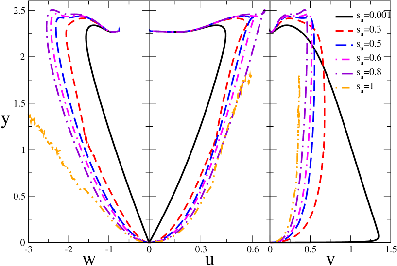
FIG. 1.: Projections of the RG flow for the three-component case, $M=3$, in the $y$-$w$, $y$-$v$ and $y$-$u$ planes, as a function of $s_{u}\equiv u_{0}/v_{0}$, for $u_{0}>0$, $v_{0}>0$, and $w_{0}<0$. Here $y_{0}=0$ and $3u_{0}+w_{0}=0$. The REIM FP corresponds to $u^{*}=v^{*}=0$, $w^{*}\approx-0.7$, and $y^{*}\approx 2.3$ (Ref. [24]).

In this Section we report our analyses of the five-loop perturbative series. We have resummed the $\beta$-functions by using the Padé-Borel method. The major numerical problem we faced was the fact that most of the approximants were defective in some region of the coupling space, forbidding a complete study of the RG flow. This is not unexpected since the perturbative series are not Borel summable. Approximant [3/1] for $\beta_{u}$, [4/1] for $\beta_{v}$, and [3/2] for $\beta_{w}$ with $b=1$ [40] were not defective in all the region of the RG flow we considered (in some cases the Padé approximant to the Borel transform had a pole on the positive real axis but far from the origin, in a region that gives a negligible contribution to the resummed function). On the other hand, all approximants for $\beta_{y}$ were defective somewhere in the region we wished to investigate. For $\beta_{y}$ we used approximant [3/2] with $b=1$, that had the least extended defective region. All results we present here were obtained by using these approximants. It must be stressed that other choices gave results that were similar in the regions in which they were well-defined.

First, we checked the general results reported in Sec. III. We considered the O($M$), cubic, O(0), and REIM FP’s and for each of them we determined the stability eigenvalues. The results are in full agreement with the conclusions of Sec. III, confirming that the O(0) and the REIM FP’s are stable. Then, we looked for additional FP’s beside those identified by the $\epsilon$-expansion analysis of Sec. III A. For this purpose we considered the RG flow starting from arbitrary values of $u,v,w,y$. We only observed runaways trajectories or a flow towards either the REIM or the O($0$) FP’s, confirming that the REIM and the O($0$) are the only stable FP’s. In particular, trajectories corresponding to Hamiltonian parameters $w_{0}<0$, $u_{0}>0$, $u_{0}+w_{0}<0$, and that satisfy the stability bound (32) never flow towards the O($0$) FP, which is therefore not accessible from this region. They either flow towards the REIM FP or apparently run away towards infinity.

For the purpose of illustration, we first consider the case $y_{0}=0$, $w_{0}/u_{0}=-M$, and $v_{0}>0$, which apparently corresponds to the model (6) with distribution (2), cf. Eq. (21) (note that $B=1/M$ in this case). In Fig. 1 we show the RG trajectories for $M=3$ for several values of $s_{u}>0$. The approximant of $\beta_{y}$ is defective for $0.05\lesssim s_{u}\lesssim 0.3$ and $y$ close to 1. This explains the sudden change of direction of the trajectory with $s_{u}=0.3$ in Fig. 1 when $y$ is close to 1. For $M=3$ (resp. $M=2$) the RG trajectories appear to approach the REIM FP for $0<s_{u}\lesssim 0.9$ (resp. $0<s_{u}\lesssim 1.4$). For larger values of $s_{u}$ the flow runs close to regions in which some approximant is defective. Apparently, trajectories flow towards infinity, but this could be an artifact of the resummation. In any case, if true, this would imply that the corresponding systems do not undergo a continuous transition. As a consequence, since $s_{u}$ is directly related to the anisotropy strength $D$, the continuous transition would be expected to disappear for sufficiently large values of $D$. These conclusions do not immediately apply to fixed-length spin systems, i.e. to the Hamiltonian (1) since in this case [41] $v_{0}=+\infty$. Thus, it is not clear which is the correct value of $s_{u}$ even for $u_{0}=\infty$. The critical behavior of this system for strong disorder has been discussed in Sec. III D.

The qualitative picture does not change if we do not require $w_{0}/u_{0}=-M$ and $s_{y}=0$. For instance, we can consider the case $w_{0}/u_{0}=-M$, $v_{0}>0$, and arbitrary $s_{y}$. We are able to resum reliably the perturbative series for $s_{y}>-0.7$ and there we observe that some trajectories flow towards the REIM FP, while others run away to infinity. The attraction domain of the REIM FP enlarges with increasing $s_{y}$: it is approximarely bounded by $s_{u}\lesssim 0.9+0.6s_{y}$ for $M=3$ ($s_{u}\lesssim 1.4+1.4s_{y}$ for $M=2$) in the region $-0.6\lesssim s_{y}\lesssim 0.3$ ($-0.7\lesssim s_{y}\lesssim 1$). For larger value of $s_{y}$, the attraction domain becomes even larger and extends beyond the lines reported above. For $s_{y}\lesssim-0.6$ some approximants become defective and we cannot determine reliably the RG flow. As in the case $s_{y}=0$, there is some evidence that trajectories flow towards infinity for $s_{y}\lesssim-1$, while for $-1\lesssim s_{y}\lesssim-0.6$ they may still flow to the REIM FP.

Then, we have investigated the behavior for $v_{0}<0$, although this region does not appear to be of physical interest. As in the pure case, all trajectories apparently run away to infinity.

Finally, let us discuss whether O($0$) critical behavior can be observed by appropriately tuning the model parameters. We have investigated this question in detail. We find that the O($0$) FP can be reached only if $u_{0}+w_{0}>0$, irrespective of the other parameters as long as $u_{0}>0$ and $w_{0}<0$. This result can be proved straightforwardly in the limiting case $v_{0}=0$. Indeed, since $\beta_{v}=0$ for $v=0$, if we start with $v_{0}=0$ the flow will be confined in the hyperplane $v=0$. But for $v=0$ we can use identities (51) that show that the flow for the couplings $u+w$ and $y$ is identical to the flow observed in the random-exchange $\varphi^{4}$ theory. Therefore, for $u_{0}+w_{0}=0$ we observe pure Ising behavior, while for $u_{0}+w_{0}<0$ (resp. $u_{0}+w_{0}>0$) RG trajectories flow towards the REIM (resp. O($0$)) FP. Therefore, if $w_{0}/u_{0}<-1$, as implied by Eq. (25), only REIM critical behavior can be observed. For $v_{0}>0$, similar conclusions are obtained numerically: The attraction domain of the O($0$) FP is included in the region $w_{0}/u_{0}>-c$, where the constant $c$ is positive and smaller than 1, depends on $s_{w}$, and tends to 1 as $s_{w}\to-\infty$, i.e. $v_{0}\to 0$.

In conclusion, our analysis gives a full picture of the critical behavior for cubic magnets that have $v_{0}>0$—we have $v_{0}=+\infty$ for fixed-length spins [41]. For $M=2$ the pure system has a critical XY transition for $s_{y}>-2/3$, an Ising transition for $s_{y}=-2/3$, and a first-order transition for $-1<s_{y}<-2/3$ [values of the parameters such that $s_{y}\leq-1$ are not allowed since they do not satisfy the stability bound (32)]. Note that first-order transitions cannot be observed in the pure model (18) with fixed-length spins. Indeed, for the strongest possible negative anisotropy, $K=-\infty$, the Hamiltonian can be written as two decoupled Ising models [42], and thus the system with $K=-\infty$ exactly corresponds to $s_{y}=-2/3$. As a consequence, finite values of $K$ have $s_{y}>-2/3$, and therefore the model is expected to have always an XY transition. Randomness changes the critical behavior. For small randomness and small anisotropy, we always predict REIM critical behavior, while for large disorder (unless we consider fixed-length spins, cf. Sec. III D) we do not expect a continuous transition. Note that the behavior of systems with $-1<s_{y}<-2/3$ remains unclear since in this region we are not able to resum reliably the perturbative expansions. In particular, we cannot clarify if softening occurs. A Monte Carlo simulation  [43] found that model (18) with $K=-\infty$ has a continuous transition for small disorder, in agreement with our results.

For $M=3$ we expect a continuous transition for $s_{y}\geq 0$ and a first-order one for $s_{y}<0$. If we add randomness to systems with $s_{y}>0$, the continuous transition survives but now belongs to the REIM universality class; for large disorder the transition may disappear. For $s_{y}<0$ one may observe softening, i.e. the first-order transition may be changed into a continuous one by small disorder. Note that softening always occurs for infinite disorder, $D_{0}=+\infty$, in the model (5), independently of the sign of $y_{0}$, under mild assumptions on the distribution $P(q)$, see Sec. III D.

A Renormalization-group dimensions of bilinear operators in the cubic-symmetric $\mathbf{\Phi^{4}}$ theory

In this appendix we compute the RG dimensions of bilinear operators in the cubic-symmetric theory

$${\cal H}_{c}=\int d^{d}x\left\{{1\over 2}(\partial_{\mu}\varphi(x))^{2}+{1\over 2}r\varphi(x)^{2}+{1\over 4!}u_{0}\left[\varphi(x)^{2}\right]^{2}+{1\over 4!}v_{0}\sum_{i=1}^{N}\varphi_{i}(x)^{4}\right\},$$ (A1)

where $\varphi$ is an $N$-component field. The bilinear operators can be written in terms of tensors belonging to different irreducible representations of the cubic group:

$$E=\frac{1}{N}\sum_{k}\varphi_{k}^{2},$$ (A2)

$$U_{i}=\varphi_{i}^{2}-\frac{1}{N}\sum_{k}\varphi_{k}^{2},$$ (A3)

$$T_{ij}=\varphi_{i}\varphi_{j},\quad i\neq j.$$ (A4)

The RG dimension of the energy operator $E$ is $y_{E}=1/\nu$, where $\nu$ is the correlation-length exponent. The RG dimensions of the operators $U_{i}$ and $T_{ij}$, respectively $y_{U}$ and $y_{T}$, in the cubic-symmetric theory (A1) will be computed below. Note that in O($N$)-symmetric theories the tensors $U_{i}$ and $T_{ij}$ belong to the same irreducible representation and therefore $y_{T}=y_{U}$. In cubic systems this is no longer the case.

In order to compute $y_{U}$ and $y_{T}$, we consider the perturbative approach in terms of the zero-momentum quartic couplings $u$ and $v$ at fixed dimension. We refer the reader to Ref. [27] for notations and definitions; there one can also find the six-loop perturbative expansion of the $\beta$-functions and of the RG functions associated with the standard exponents. In order to compute the RG dimensions of $U_{i}$ and $T_{ij}$, we consider the related RG functions $Z_{U}$ and $Z_{T}$, defined in terms of the zero-momentum one-particle irreducible two-point functions $\Gamma_{U}^{(2)}(0)$ and $\Gamma_{T}^{(2)}(0)$ with an insertion of the operator $U_{i}$ and $T_{ij}$, respectively, i.e.

$$\Gamma_{U}^{(2)}(0)_{i,kl}=Z_{U}^{-1}\;B_{i,kl},\qquad\Gamma_{T}^{(2)}(0)_{ij,kl}=Z_{T}^{-1}\;A_{ij,kl},$$ (A5)

where $B$ and $A$ are appropriate constant tensors such that $Z_{U}=Z_{T}=1$ at tree level. Then, we compute the RG functions $\eta_{U}$ and $\eta_{T}$ defined by

$$\eta_{U,T}(u,v)=\left.{\partial\ln Z_{U,T}\over\partial\ln m}\right|_{u_{0},v_{0}}=\beta_{u}{\partial\ln Z_{U,T}\over\partial u}+\beta_{v}{\partial\ln Z_{U,T}\over\partial v},$$ (A6)

where $\beta_{u}$ and $\beta_{v}$ are the $\beta$-functions.

We computed the functions $\Gamma^{(2)}_{U,T}(0)$ to six loops. The resulting six-loop series of $\eta_{U,T}(u,v)$ are

$$\eta_{U}(u,v)=-\frac{2u}{8+N}-\frac{1}{3}v+u^{2}\frac{12+2N}{3(8+N)^{2}}+\frac{4}{3(N+8)}uv+\frac{2}{27}v^{2}+\sum_{ij}e^{U}_{ij}u^{i}v^{j},$$ (A7)

$$\eta_{T}(u,v)=-\frac{2u}{8+N}+u^{2}\frac{12+2N}{3(8+N)^{2}}+\frac{4}{9(N+8)}uv+u\sum_{ij}e^{T}_{ij}u^{i}v^{j},$$ (A8)

where $u$ and $v$ are normalized so that

$$mu={8+M\over 48\pi}Z_{u}u_{0},\qquad mv={3\over 16\pi}Z_{v}v_{0},\qquad Z_{u,v}=1+O(u,v),$$ (A9)

and the coefficients $e^{U}_{ij}$ an $e^{T}_{ij}$ are reported in Tables X and XI respectively. Note that $u$ and $v$ correspond to $\bar{u}$ and $\bar{v}$ in Ref. [27]. The RG dimensions $y_{U}$ and $y_{T}$ are obtained by $y_{U,T}=2+\eta_{U,T}-\eta$, where $\eta_{U,T}$ is the value obtained by resumming the corresponding series, evaluating it at $u=u^{*}$, $v=v^{*}$, where ($u^{*}$,$v^{*}$) is the stable FP.

In the case of the REIM, i.e., in the limit $N\rightarrow 0$, one has $y_{U}=y_{E}=1/\nu$. Indeed, $\langle\varphi_{i}^{2}\varphi_{k}\varphi_{l}\rangle^{1PI}$ and $\langle\sum_{i}\varphi_{i}^{2}\varphi_{k}\varphi_{l}\rangle^{1PI}$ are both finite and nonvanishing for $N\to 0$. Therefore, we have for $N\to 0$

$$\langle NU_{i}\varphi_{k}\varphi_{l}\rangle^{1PI}=-\langle\sum_{j}\varphi_{j}^{2}\varphi_{k}\varphi_{l}\rangle^{1PI}+O(N)=-\langle NE\varphi_{k}\varphi_{l}\rangle^{1PI}+O(N).$$ (A10)

Using the Monte Carlo estimate $\nu=0.683(3)$ (Ref. [19]), we obtain $y_{U}=1.464(6)$. The series for $\eta_{T}$ was already reported in Ref. [44]. Its analysis provided the estimate $y_{T}=2.08(3)$.

For $N=2$ the stable FP of the cubic theory is the O(2) FP, so $y_{U}=y_{T}=1.766(3)$ [26]. For $N\geq 3$ the O($N$) FP is unstable and the RG trajectories flow toward another FP characterized by a discrete cubic symmetry. The analysis of the series, using the same procedure reported in Ref. [27], gives the estimates

$$y_{U}(N=3)=1.774(7),\qquad y_{T}(N=3)=1.800(2),$$ (A11)

$$y_{U}(N=4)=1.696(8),\qquad y_{T}(N=4)=1.874(3).$$ (A12)

B Some renormalization-group identities

In this Appendix we prove relations (51). Morever, we show that, in the limit $N\to 0$, the RG functions do not depend on $M$ for $v=0$.

Let us consider the Hamiltonian for $v_{0}=0$ and rewrite

$$\exp\left[-{1\over 4!}\sum_{ij,ab}(u_{0}+w_{0}\delta_{ab}+y_{0}\delta_{ab}\delta_{ij})\phi^{2}_{ai}\phi^{2}_{bj}\right]\sim\int d\lambda d\rho_{a}d\sigma_{ai}$$ (B1)

$$\qquad\exp\left[{1\over 2}(\lambda^{2}+\sum_{a}\rho_{a}^{2}+\sum_{ai}\sigma_{ai}^{2})+{1\over 2\sqrt{3}}\sum_{ai}(\sqrt{u_{0}}\lambda+\sqrt{w_{0}}\rho_{a}+\sqrt{y_{0}}\sigma_{ai})\phi_{ai}^{2}\right],$$ (B2)

where $a$ (resp. $i$) runs from 1 to $M$ (resp. $N$) and $\lambda$, $\rho_{a}$, and $\sigma_{ai}$ are auxiliary fields. Then, let us consider the $n$-point irreducible correlation function. We will show that it has the form

$$\langle\phi_{a_{1}i_{1}}\ldots\phi_{a_{n}i_{n}}\rangle=\sum_{\alpha}c_{\alpha}Q_{\alpha}^{{a_{1}i_{1}}\ldots{a_{n}i_{n}}},$$ (B3)

where $Q_{\alpha}$ are group tensors (products of Kronecker deltas), the scalar factors $c_{\alpha}$ do not depend on $M$, and the sum runs over all possible independent group tensors. In terms of the auxiliary fields, Feynman diagrams contain loops of $\phi$-fields and $n/2$ open lines of $\phi$-fields connected by the auxiliary-field lines. The group factor associated with each diagram is computed as follows. One assigns indices $ai$ to $\phi$ and $\sigma$ propagators and indices $a$ to $\rho$ propagators, considers the product of the factors $V$ (reported below) associated with each vertex, and sums over all assigned indices. In order to prove the $M$-independence we will show that, because of the Kronecker $\delta$’s appearing in the diagrams, none of these sums is effectively performed in the limit $N\to 0$, so that no factor of $M$ can appear. The factors $V$ are given by:

$$V(\lambda,\phi_{ai},\phi_{bj})={\sqrt{u_{0}}\over\sqrt{3}}\delta_{ab}\delta_{ij},$$ (B4)

$$V(\rho_{c},\phi_{ai},\phi_{bj})={\sqrt{w_{0}}\over\sqrt{3}}\delta_{abc}\delta_{ij},$$ (B5)

$$V(\sigma_{ck},\phi_{ai},\phi_{bj})={\sqrt{y_{0}}\over\sqrt{3}}\delta_{abc}\delta_{ijk},$$ (B6)

where $abc$ (resp. $ijk$) run from 1 to $M$ (resp. $N$). First, note that all $\phi$ loops must contain at least a $\sigma\phi\phi$ vertex, otherwise by summing over the indices of the $\phi$ fields appearing in the loop one obtains a factor of $N$. As a consequence, all loops give rise to a very simple effective vertex for the auxiliary fields:

$$\langle\lambda\ldots\lambda\rho_{a_{1}}\ldots\rho_{a_{n}}\sigma_{b_{1}i_{1}}\ldots\sigma_{b_{m}i_{m}}\rangle\sim\delta_{a_{1}\ldots a_{n}b_{1}\ldots b_{m}}\delta_{i_{1}\ldots i_{m}},$$ (B7)

where we have only written the dependence on the group indices. Then, given a diagram, let us consider the reduced diagram in which all $\phi$ loops are replaced by the corresponding effective vertices. The $\sigma_{ai}$ propagators form several connected paths. It is easy to convince oneself that each of these paths must end at an open $\phi$ line, otherwise, by summing over the indices $i$ associated with the $\sigma$ lines, one obtains factors of $N$. As a consequence, all effective vertices are connected by $\sigma$ propagators to the open $\phi$ lines. Therefore, by summing over the indices associated with the $\phi$ and $\sigma$ propagators one obtains expressions in which all remaining indices (those related to $\rho$ propagators) are equal to external ones and are not summed over. We have thus proved that correlation functions expressed in terms of the bare parameters do not depend on $M$. Since $R_{MN}$ is $M$ independent for $N\to 0$, this result extends trivially to the RG functions expressed in terms of the renormalized couplings.

To prove identities (51) we now exploit the $M$ independence. For $M=1$ the theory corresponds to the REIM model with couplings $u_{0}+w_{0}$ and $y_{0}$. Since $R_{MN}=R_{N}$ for $N\to 0$, $(u+v)/m$ is a function of $u_{0}+w_{0}$. The result follows immediately.

TABLE II.: The five-loop series of $\beta_{u}=m\partial u/\partial m$ for $M=3$. Setting $\beta_{u}\equiv\sum_{l=0}\beta_{u,l}$, where $l$ is the number of loops, we report $\beta_{u,l}$ up to $l=5$.

$l$	$\beta_{u,l}$
0	$-u$
1	$u^{2}+\frac{10}{11}u\,v+\frac{1}{2}u\,w+\frac{2}{11}v\,w+\frac{2}{3}u\,y$
2	$-\frac{95}{216}u^{3}-\frac{250}{297}u^{2}\,v-\frac{460}{3267}u\,v^{2}-\frac{25}{54}u^{2}\,w-\frac{41}{99}u\,v\,w-\frac{8}{363}v^{2}\,w-\frac{23}{216}u\,w^{2}-\frac{1}{33}v\,w^{2}-\frac{50}{81}u^{2}\,y-\frac{184}{891}u\,v\,y-\frac{23}{81}u\,w\,y-\frac{92}{729}u\,y^{2}$
3	$0.389923\,u^{4}+1.16913\,u^{3}\,v+0.621933\,u^{2}\,v^{2}+0.10714\,u\,v^{3}+0.64302\,u^{3}\,w+1.1669\,u^{2}\,v\,w+0.41177\,u\,v^{2}\,w+0.02168\,v^{3}\,w$
	$+0.35637\,u^{2}\,w^{2}+0.394263\,u\,v\,w^{2}+0.048431\,v^{2}\,w^{2}+0.0730773\,u\,w^{3}+0.0254122\,v\,w^{3}+0.857364\,u^{3}\,y+0.912169\,u^{2}\,v\,y$
	$+0.235717\,u\,v^{2}\,y+0.95032\,u^{2}\,w\,y+0.597082\,u\,v\,w\,y+0.023813\,v^{2}\,w\,y+0.292309\,u\,w^{2}\,y+0.0327432\,v\,w^{2}\,y+0.46739\,u^{2}\,y^{2}$
	$+0.230387\,u\,v\,y^{2}+0.299507\,u\,w\,y^{2}+0.00418781\,v\,w\,y^{2}+0.090449\,u\,y^{3}$
4	$-0.447316\,u^{5}-1.83254\,u^{4}\,v-1.7466\,u^{3}\,v^{2}-0.575817\,u^{2}\,v^{3}-0.076344\,u\,v^{4}-1.0079\,u^{4}\,w-2.83639\,u^{3}\,v\,w-1.9044\,u^{2}\,v^{2}\,w$
	$-0.380099\,u\,v^{3}\,w-0.0145582\,v^{4}\,w-0.885278\,u^{3}\,w^{2}-1.74084\,u^{2}\,v\,w^{2}-0.695073\,u\,v^{2}\,w^{2}-0.038822\,v^{3}\,w^{2}-0.37419\,u^{2}\,w^{3}$
	$-0.451159\,u\,v\,w^{3}-0.0547698\,v^{2}\,w^{3}-0.06557\,u\,w^{4}-0.0232153\,v\,w^{4}-1.34386\,u^{4}\,y-2.56167\,u^{3}\,v\,y-1.2668\,u^{2}\,v^{2}\,y$
	$-0.223943\,u\,v^{3}\,y-2.36074\,u^{3}\,w\,y-3.0627\,u^{2}\,v\,w\,y-0.87616\,u\,v^{2}\,w\,y-0.023185\,v^{3}\,w\,y-1.49676\,u^{2}\,w^{2}\,y-1.14351\,u\,v\,w^{2}\,y$
	$-0.0520405\,v^{2}\,w^{2}\,y-0.349706\,u\,w^{3}\,y-0.0459449\,v\,w^{3}\,y-1.2213\,u^{3}\,y^{2}-1.23262\,u^{2}\,v\,y^{2}-0.32717\,u\,v^{2}\,y^{2}-1.5635\,u^{2}\,w\,y^{2}$
	$-0.888055\,u\,v\,w\,y^{2}-0.0135895\,v^{2}\,w\,y^{2}-0.550107\,u\,w^{2}\,y^{2}-0.0186856\,v\,w^{2}\,y^{2}-0.476234\,u^{2}\,y^{3}-0.252712\,u\,v\,y^{3}$
	$-0.335525\,u\,w\,y^{3}-0.00289791\,v\,w\,y^{3}-0.0754467\,u\,y^{4}$
5	$0.633855\,u^{6}+3.32208\,u^{5}\,v+4.6464\,u^{4}\,v^{2}+2.53461\,u^{3}\,v^{3}+0.702909\,u^{2}\,v^{4}+0.0816358\,u\,v^{5}+1.82714\,u^{5}\,w+7.04207\,u^{4}\,v\,w$
	$+7.40684\,u^{3}\,v^{2}\,w+2.97466\,u^{2}\,v^{3}\,w+0.499013\,u\,v^{4}\,w+0.0162882\,v^{5}\,w+2.22077\,u^{4}\,w^{2}+6.4639\,u^{3}\,v\,w^{2}+4.81333\,u^{2}\,v^{2}\,w^{2}$
	$+1.15478\,u\,v^{3}\,w^{2}+0.0555485\,v^{4}\,w^{2}+1.45911\,u^{3}\,w^{3}+3.06664\,u^{2}\,v\,w^{3}+1.35727\,u\,v^{2}\,w^{3}+0.0935349\,v^{3}\,w^{3}+0.522432\,u^{2}\,w^{4}$
	$+0.661835\,u\,v\,w^{4}+0.0871471\,v^{2}\,w^{4}+0.0804704\,u\,w^{5}+0.0286439\,v\,w^{5}+2.43619\,u^{5}\,y+6.81471\,u^{4}\,v\,y+5.57615\,u^{3}\,v^{2}\,y$
	$+2.06187\,u^{2}\,v^{3}\,y+0.29933\,u\,v^{4}\,y+5.92205\,u^{4}\,w\,y+12.266\,u^{3}\,v\,w\,y+7.27261\,u^{2}\,v^{2}\,w\,y+1.54143\,u\,v^{3}\,w\,y+0.037268\,v^{4}\,w\,y$
	$+5.83645\,u^{3}\,w^{2}\,y+8.62368\,u^{2}\,v\,w^{2}\,y+2.93576\,u\,v^{2}\,w^{2}\,y+0.111143\,v^{3}\,w^{2}\,y+2.7863\,u^{2}\,w^{3}\,y+2.37933\,u\,v\,w^{3}\,y$
	$+0.148969\,v^{2}\,w^{3}\,y+0.53647\,u\,w^{4}\,y+0.0809503\,v\,w^{4}\,y+3.14287\,u^{4}\,y^{2}+5.2433\,u^{3}\,v\,y^{2}+2.89085\,u^{2}\,v^{2}\,y^{2}+0.557283\,u\,v^{3}\,y^{2}$
	$+6.20834\,u^{3}\,w\,y^{2}+7.3735\,u^{2}\,v\,w\,y^{2}+2.24663\,u\,v^{2}\,w\,y^{2}+0.034735\,v^{3}\,w\,y^{2}+4.45664\,u^{2}\,w^{2}\,y^{2}+2.95624\,u\,v\,w^{2}\,y^{2}$
	$+0.0805995\,v^{2}\,w^{2}\,y^{2}+1.14677\,u\,w^{3}\,y^{2}+0.0642921\,v\,w^{3}\,y^{2}+1.93839\,u^{3}\,y^{3}+2.12342\,u^{2}\,v\,y^{3}+0.61093\,u\,v^{2}\,y^{3}$
	$+2.79532\,u^{2}\,w\,y^{3}+1.66738\,u\,v\,w\,y^{3}+0.0148483\,v^{2}\,w\,y^{3}+1.08348\,u\,w^{2}\,y^{3}+0.020416\,v\,w^{2}\,y^{3}+0.630396\,u^{2}\,y^{4}$
	$+0.362335\,u\,v\,y^{4}+0.489119\,u\,w\,y^{4}+0.0022041\,v\,w\,y^{4}+0.0874933\,u\,y^{5}$

TABLE III.: The five-loop series of $\beta_{v}=m\partial v/\partial m$ for $M=3$. Setting $\beta_{v}\equiv\sum_{l=0}\beta_{v,l}$, where $l$ is the number of loops, we report $\beta_{v,l}$ up to $l=5$.

$l$	$\beta_{v,l}$
0	$-v$
1	$\frac{3\,u\,v}{2}+v^{2}+\frac{v\,w}{2}+\frac{2\,v\,y}{3}$
2	$-\frac{185\,u^{2}\,v}{216}-\frac{412\,u\,v^{2}}{297}-\frac{1252\,v^{3}}{3267}-\frac{77\,u\,v\,w}{108}-\frac{47\,v^{2}\,w}{99}-\frac{23\,v\,w^{2}}{216}-\frac{77\,u\,v\,y}{81}-\frac{400\,v^{2}\,y}{891}-\frac{23\,v\,w\,y}{81}-\frac{92\,v\,y^{2}}{729}$
3	$0.916668\,u^{3}\,v+2.35093\,u^{2}\,v^{2}+1.40888\,u\,v^{3}+0.28295\,v^{4}+1.2163\,u^{2}\,v\,w+1.79079\,u\,v^{2}\,w+0.542156\,v^{3}\,w+0.49351\,u\,v\,w^{2}$
	$+0.367154\,v^{2}\,w^{2}+0.0730773\,v\,w^{3}+1.62177\,u^{2}\,v\,y+1.7731\,u\,v^{2}\,y+0.508415\,v^{3}\,y+1.31602\,u\,v\,w\,y+0.746208\,v^{2}\,w\,y$
	$+0.292309\,v\,w^{2}\,y+0.63527\,u\,v\,y^{2}+0.346201\,v^{2}\,y^{2}+0.299507\,v\,w\,y^{2}+0.090449\,v\,y^{3}$
4	$-1.22868\,u^{4}\,v-4.3522\,u^{3}\,v^{2}-4.33525\,u^{2}\,v^{3}-1.75357\,u\,v^{4}-0.270333\,v^{5}-2.26103\,u^{3}\,v\,w-5.40209\,u^{2}\,v^{2}\,w-3.5142\,u\,v^{3}\,w$
	$-0.712012\,v^{4}\,w-1.53326\,u^{2}\,v\,w^{2}-2.40612\,u\,v^{2}\,w^{2}-0.798138\,v^{3}\,w^{2}-0.486101\,u\,v\,w^{3}-0.401462\,v^{2}\,w^{3}-0.06557\,v\,w^{4}$
	$-3.0147\,u^{3}\,v\,y-5.65057\,u^{2}\,v^{2}\,y-3.27089\,u\,v^{3}\,y-0.650693\,v^{4}\,y-4.0887\,u^{2}\,v\,w\,y-5.03042\,u\,v^{2}\,w\,y-1.47787\,v^{3}\,w\,y$
	$-1.9444\,u\,v\,w^{2}\,y-1.26296\,v^{2}\,w^{2}\,y-0.349706\,v\,w^{3}\,y-2.1004\,u^{2}\,v\,y^{2}-2.31802\,u\,v^{2}\,y^{2}-0.671001\,v^{3}\,y^{2}-2.02679\,u\,v\,w\,y^{2}$
	$-1.16492\,v^{2}\,w\,y^{2}-0.550107\,v\,w^{2}\,y^{2}-0.616942\,u\,v\,y^{3}-0.350699\,v^{2}\,y^{3}-0.335525\,v\,w\,y^{3}-0.0754467\,v\,y^{4}$
5	$1.97599\,u^{5}\,v+9.00629\,u^{4}\,v^{2}+12.7239\,u^{3}\,v^{3}+7.96583\,u^{2}\,v^{4}+2.46634\,u\,v^{5}+0.312556\,v^{6}+4.69417\,u^{4}\,v\,w+15.6644\,u^{3}\,v^{2}\,w$
	$+16.0384\,u^{2}\,v^{3}\,w+6.69086\,u\,v^{4}\,w+1.04399\,v^{5}\,w+4.50574\,u^{3}\,v\,w^{2}+11.0238\,u^{2}\,v^{2}\,w^{2}+7.53313\,u\,v^{3}\,w^{2}+1.60193\,v^{4}\,w^{2}$
	$+2.28761\,u^{2}\,v\,w^{3}+3.82594\,u\,v^{2}\,w^{3}+1.35045\,v^{3}\,w^{3}+0.642513\,u\,v\,w^{4}+0.562428\,v^{2}\,w^{4}+0.0804704\,v\,w^{5}+6.25889\,u^{4}\,v\,y$
	$+16.8745\,u^{3}\,v^{2}\,y+15.2053\,u^{2}\,v^{3}\,y+6.1052\,u\,v^{4}\,y+0.947895\,v^{5}\,y+12.0153\,u^{3}\,v\,w\,y+23.5313\,u^{2}\,v^{2}\,w\,y+14.2714\,u\,v^{3}\,w\,y$
	$+2.9145\,v^{4}\,w\,y+9.15043\,u^{2}\,v\,w^{2}\,y+12.2315\,u\,v^{2}\,w^{2}\,y+3.8419\,v^{3}\,w^{2}\,y+3.42673\,u\,v\,w^{3}\,y+2.40324\,v^{2}\,w^{3}\,y+0.53647\,v\,w^{4}\,y$
	$+6.36312\,u^{3}\,v\,y^{2}+11.045\,u^{2}\,v^{2}\,y^{2}+6.4832\,u\,v^{3}\,y^{2}+1.31809\,v^{4}\,y^{2}+9.71176\,u^{2}\,v\,w\,y^{2}+11.5283\,u\,v^{2}\,w\,y^{2}+3.48488\,v^{3}\,w\,y^{2}$
	$+5.47297\,u\,v\,w^{2}\,y^{2}+3.4119\,v^{2}\,w^{2}\,y^{2}+1.14677\,v\,w^{3}\,y^{2}+3.01986\,u^{2}\,v\,y^{3}+3.47764\,u\,v^{2}\,y^{3}+1.04671\,v^{3}\,y^{3}+3.42367\,u\,v\,w\,y^{3}$
	$+2.05758\,v^{2}\,w\,y^{3}+1.08348\,v\,w^{2}\,y^{3}+0.771673\,u\,v\,y^{4}+0.461776\,v^{2}\,y^{4}+0.489119\,v\,w\,y^{4}+0.0874933\,v\,y^{5}$

TABLE IV.: The five-loop series of $\beta_{w}=m\partial w/\partial m$ for $M=3$. Setting $\beta_{w}\equiv\sum_{l=0}\beta_{w,l}$, where $l$ is the number of loops, we report $\beta_{w,l}$ up to $l=5$.

$l$	$\beta_{w,l}$
0	$-w$
1	$\frac{3\,u\,w}{2}+\frac{4\,v\,w}{11}+w^{2}+\frac{2\,w\,y}{3}$
2	$-\frac{185\,u^{2}\,w}{216}-\frac{223\,u\,v\,w}{297}-\frac{244\,v^{2}\,w}{3267}-\frac{131\,u\,w^{2}}{108}-\frac{47\,v\,w^{2}}{99}-\frac{95\,w^{3}}{216}-\frac{77\,u\,w\,y}{81}-\frac{184\,v\,w\,y}{891}-\frac{50\,w^{2}\,y}{81}-\frac{92\,w\,y^{2}}{729}$
3	$0.916668\,u^{3}\,w+1.37496\,u^{2}\,v\,w+0.362132\,u\,v^{2}\,w+0.042103\,v^{3}\,w+1.98317\,u^{2}\,w^{2}+1.74277\,u\,v\,w^{2}+0.271146\,v^{2}\,w^{2}$
	$+1.48661\,u\,w^{3}+0.676067\,v\,w^{3}+0.389923\,w^{4}+1.62177\,u^{2}\,w\,y+0.939981\,u\,v\,w\,y+0.164277\,v^{2}\,w\,y+2.27978\,u\,w^{2}\,y$
	$+0.732074\,v\,w^{2}\,y+0.857364\,w^{3}\,y+0.63527\,u\,w\,y^{2}+0.217823\,v\,w\,y^{2}+0.467389\,w^{2}\,y^{2}+0.090449\,w\,y^{3}$
4	$-1.22868\,u^{4}\,w-2.66348\,u^{3}\,v\,w-1.4268\,u^{2}\,v^{2}\,w-0.347251\,u\,v^{3}\,w-0.0326696\,v^{4}\,w-3.58788\,u^{3}\,w^{2}-5.25808\,u^{2}\,v\,w^{2}$
	$-1.93572\,u\,v^{2}\,w^{2}-0.244281\,v^{3}\,w^{2}-4.09897\,u^{2}\,w^{3}-3.9245\,u\,v\,w^{3}-0.759482\,v^{2}\,w^{3}-2.17101\,u\,w^{4}-1.07631\,v\,w^{4}$
	$-0.447316\,w^{5}-3.0147\,u^{3}\,w\,y-3.33336\,u^{2}\,v\,w\,y-1.18975\,u\,v^{2}\,w\,y-0.154387\,v^{3}\,w\,y-6.5664\,u^{2}\,w^{2}\,y-4.83085\,u\,v\,w^{2}\,y$
	$-0.899584\,v^{2}\,w^{2}\,y-5.02574\,u\,w^{3}\,y-1.95255\,v\,w^{3}\,y-1.34386\,w^{4}\,y$
	$-2.1004\,u^{2}\,w\,y^{2}-1.46007\,u\,v\,w\,y^{2}-0.286402\,v^{2}\,w\,y^{2}-3.1138\,u\,w^{2}\,y^{2}-1.15025\,v\,w^{2}\,y^{2}-1.2213\,w^{3}\,y^{2}-0.616942\,u\,w\,y^{3}$
	$-0.244019\,v\,w\,y^{3}-0.476234\,w^{2}\,y^{3}-0.0754467\,w\,y^{4}$
5	$1.97599\,u^{5}\,w+5.70624\,u^{4}\,v\,w+4.72927\,u^{3}\,v^{2}\,w+1.77266\,u^{2}\,v^{3}\,w+0.357776\,u\,v^{4}\,w+0.0327712\,v^{5}\,w+7.28706\,u^{4}\,w^{2}$
	$+15.3337\,u^{3}\,v\,w^{2}+9.42002\,u^{2}\,v^{2}\,w^{2}+2.47241\,u\,v^{3}\,w^{2}+0.26882\,v^{4}\,w^{2}+11.2179\,u^{3}\,w^{3}+17.1513\,u^{2}\,v\,w^{3}+7.14394\,u\,v^{2}\,w^{3}$
	$+0.985494\,v^{3}\,w^{3}+8.985399\,u^{2}\,w^{4}+9.21597\,u\,v\,w^{4}+1.99704\,v^{2}\,w^{4}+3.72266\,u\,w^{5}+1.9646\,v\,w^{5}+0.633855\,w^{6}$
	$+6.25889\,u^{4}\,w\,y+10.5195\,u^{3}\,v\,w\,y+5.91865\,u^{2}\,v^{2}\,w\,y+1.6148\,u\,v^{3}\,w\,y+0.18753\,v^{4}\,w\,y+18.525\,u^{3}\,w^{2}\,y+22.759\,u^{2}\,v\,w^{2}\,y$
	$+8.91572\,u\,v^{2}\,w^{2}\,y+1.29356\,v^{3}\,w^{2}\,y+21.5756\,u^{2}\,w^{3}\,y+18.0042\,u\,v\,w^{3}\,y+3.7067\,v^{2}\,w^{3}\,y+11.6445\,u\,w^{4}\,y+5.06192\,v\,w^{4}\,y$
	$+2.43619\,w^{5}\,y+6.36312\,u^{3}\,w\,y^{2}+7.15909\,u^{2}\,v\,w\,y^{2}+2.9287\,u\,v^{2}\,w\,y^{2}+0.453078\,v^{3}\,w\,y^{2}+14.4006\,u^{2}\,w^{2}\,y^{2}$
	$+11.226\,u\,v\,w^{2}\,y^{2}+2.42873\,v^{2}\,w^{2}\,y^{2}+11.4247\,u\,w^{3}\,y^{2}+4.69358\,v\,w^{3}\,y^{2}+3.14287\,w^{4}\,y^{2}+3.01986\,u^{2}\,w\,y^{3}$
	$+0.566387\,v^{2}\,w\,y^{3}+4.73169\,u\,w^{2}\,y^{3}+2.0427\,v\,w^{2}\,y^{3}+1.93839\,w^{3}\,y^{3}+0.771673\,u\,w\,y^{4}+0.355723\,v\,w\,y^{4}+0.630396\,w^{2}\,y^{4}$
	$+2.45617\,u\,v\,w\,y^{3}+0.0874933\,w\,y^{5}$

TABLE V.: The five-loop series of $\beta_{y}=m\partial y/\partial m$ for $M=3$. Setting $\beta_{y}\equiv\sum_{l=0}\beta_{y,l}$, where $l$ is the number of loops, we report $\beta_{y,l}$ up to $l=5$.

$l$	$\beta_{y,l}$
0	$-y$
1	$\frac{9\,v\,w}{11}+\frac{3\,u\,y}{2}+\frac{12\,v\,y}{11}+\frac{3\,w\,y}{2}+y^{2}$
2	$-\frac{9\,u\,v\,w}{11}-\frac{63\,v^{2}\,w}{121}-\frac{27\,v\,w^{2}}{44}-\frac{185\,u^{2}\,y}{216}-\frac{439\,u\,v\,y}{297}-\frac{1756\,v^{2}\,y}{3267}-\frac{185\,u\,w\,y}{108}-\frac{185\,v\,w\,y}{99}$
	$-\frac{185\,w^{2}\,y}{216}-\frac{104\,u\,y^{2}}{81}-\frac{832\,v\,y^{2}}{891}-\frac{104\,w\,y^{2}}{81}-\frac{308\,y^{3}}{729}$
3	$1.25483\,u^{2}\,v\,w+1.62749\,u\,v^{2}\,w+0.44594\,v^{3}\,w+1.84622\,u\,v\,w^{2}+1.1317\,v^{2}\,w^{2}+0.690211\,v\,w^{3}+0.916668\,u^{3}\,y$
	$+2.49036\,u^{2}\,v\,y+1.80879\,u\,v^{2}\,y+0.438494\,v^{3}\,y+2.75\,u^{2}\,w\,y+5.96358\,u\,v\,w\,y+2.36751\,v^{2}\,w\,y+2.75\,u\,w^{2}\,y+3.2512\,v\,w^{2}\,y$
	$+0.91667\,w^{3}\,y+2.133\,u^{2}\,y^{2}+3.1195\,u\,v\,y^{2}+1.13436\,v^{2}\,y^{2}+4.26599\,u\,w\,y^{2}+3.38291\,v\,w\,y^{2}+2.133\,w^{2}\,y^{2}+1.47806\,u\,y^{3}$
	$+1.07495\,v\,y^{3}+1.47806\,w\,y^{3}+0.35107\,y^{4}$
4	$-2.17122\,u^{3}\,v\,w-4.35781\,u^{2}\,v^{2}\,w-2.48256\,u\,v^{3}\,w-0.48565\,v^{4}\,w-4.77724\,u^{2}\,v\,w^{2}-6.00211\,u\,v^{2}\,w^{2}-1.72925\,v^{3}\,w^{2}$
	$-3.62343\,u\,v\,w^{3}-2.2762\,v^{2}\,w^{3}-0.951639\,v\,w^{4}-1.22868\,u^{4}\,y-4.59345\,u^{3}\,v\,y-5.3004\,u^{2}\,v^{2}\,y-2.55397\,u\,v^{3}\,y$
	$-0.464358\,v^{4}\,y-4.91474\,u^{3}\,w\,y-16.2997\,u^{2}\,v\,w\,y-13.3566\,u\,v^{2}\,w\,y-3.38345\,v^{3}\,w\,y-7.37211\,u^{2}\,w^{2}\,y-17.4996\,u\,v\,w^{2}\,y$
	$-7.45225\,v^{2}\,w^{2}\,y-4.91474\,u\,w^{3}\,y-6.09451\,v\,w^{3}\,y-1.22868\,w^{4}\,y-3.89927\,u^{3}\,y^{2}-9.02889\,u^{2}\,v\,y^{2}-6.52141\,u\,v^{2}\,y^{2}$
	$-1.58095\,v^{3}\,y^{2}-11.6978\,u^{2}\,w\,y^{2}-19.0578\,u\,v\,w\,y^{2}-7.19018\,v^{2}\,w\,y^{2}-11.6978\,u\,w^{2}\,y^{2}-9.94972\,v\,w^{2}\,y^{2}-3.89927\,w^{3}\,y^{2}$
	$-4.23696\,u^{2}\,y^{3}-6.1212\,u\,v\,y^{3}-2.22589\,v^{2}\,y^{3}-8.47392\,u\,w\,y^{3}-6.37921\,v\,w\,y^{3}-4.23696\,w^{2}\,y^{3}$
	$-2.03309\,u\,y^{4}-1.47861\,v\,y^{4}-2.03309\,w\,y^{4}-0.376527\,y^{5}$
5	$4.2429179\,u^{4}\,v\,w+11.7357\,u^{3}\,v^{2}\,w+10.5256\,u^{2}\,v^{3}\,w+4.10472\,u\,v^{4}\,w+0.618728\,v^{5}\,w+12.4807\,u^{3}\,v\,w^{2}+24.3706\,u^{2}\,v^{2}\,w^{2}$
	$+14.3671\,u\,v^{3}\,w^{2}+2.82095\,v^{4}\,w^{2}+14.2955\,u^{2}\,v\,w^{3}+18.2581\,u\,v^{2}\,w^{3}+5.42606\,v^{3}\,w^{3}+7.5579084\,u\,v\,w^{4}+4.86798\,v^{2}\,w^{4}$
	$+1.55088\,v\,w^{5}+1.97599\,u^{5}\,y+9.47772\,u^{4}\,v\,y+15.161\,u^{3}\,v^{2}\,y+11.1288\,u^{2}\,v^{3}\,y+4.00642\,u\,v^{4}\,y+0.582751\,v^{5}\,y$
	$+9.87996\,u^{4}\,w\,y+44.5209\,u^{3}\,v\,w\,y+56.6807\,u^{2}\,v^{2}\,w\,y+28.7278\,u\,v^{3}\,w\,y+5.3291\,v^{4}\,w\,y+19.760\,u^{3}\,w^{2}\,y+71.398\,u^{2}\,v\,w^{2}\,y$
	$+61.8264\,u\,v^{2}\,w^{2}\,y+16.0162\,v^{3}\,w^{2}\,y+19.760\,u^{2}\,w^{3}\,y+49.2653\,u\,v\,w^{3}\,y+21.8335\,v^{2}\,w^{3}\,y+9.87996\,u\,w^{4}\,y+12.6315\,v\,w^{4}\,y$
	$+1.97599\,w^{5}\,y+7.98749\,u^{4}\,y^{2}+25.6071\,u^{3}\,v\,y^{2}+28.2134\,u^{2}\,v^{2}\,y^{2}+13.5424\,u\,v^{3}\,y^{2}+2.46225\,v^{4}\,y^{2}+31.9499\,u^{3}\,w\,y^{2}$
	$+80.4247\,u^{2}\,v\,w\,y^{2}+60.7793\,u\,v^{2}\,w\,y^{2}+14.9778\,v^{3}\,w\,y^{2}+47.9249\,u^{2}\,w^{2}\,y^{2}+82.7197\,u\,v\,w^{2}\,y^{2}+32.0629\,v^{2}\,w^{2}\,y^{2}$
	$+31.9499\,u\,w^{3}\,y^{2}+28.2945\,v\,w^{3}\,y^{2}+7.98749\,w^{4}\,y^{2}+11.9097\,u^{3}\,y^{3}+26.2915\,u^{2}\,v\,y^{3}+18.9292\,u\,v^{2}\,y^{3}+4.58889\,v^{3}\,y^{3}$
	$+35.729\,u^{2}\,w\,y^{3}+53.9545\,u\,v\,w\,y^{3}+19.9234\,v^{2}\,w\,y^{3}+35.729\,u\,w^{2}\,y^{3}+27.6713\,v\,w^{2}\,y^{3}+11.9097\,w^{3}\,y^{3}+8.72598\,u^{2}\,y^{4}$
	$+12.5648\,u\,v\,y^{4}+4.56903\,v^{2}\,y^{4}+17.452\,u\,w\,y^{4}+12.881\,v\,w\,y^{4}+8.72598\,w^{2}\,y^{4}+3.24652\,u\,y^{5}+2.3611\,v\,y^{5}+3.24652\,w\,y^{5}$
	$+0.495548\,y^{6}$

TABLE VI.: The five-loop series of $\beta_{u}=m\partial u/\partial m$ for $M=2$. Setting $\beta_{u}\equiv\sum_{l=0}\beta_{u,l}$, where $l$ is the number of loops, we report $\beta_{u,l}$ up to $l=5$.

$l$	$\beta_{u,l}$
0	$-u$
1	$u^{2}+\frac{4}{5}uv+\frac{1}{2}uw+\frac{1}{5}vw+\frac{2}{3}uy$
2	$-\frac{95\,u^{3}}{216}-\frac{20\,u^{2}\,v}{27}-\frac{92\,u\,v^{2}}{675}-\frac{25\,u^{2}\,w}{54}-\frac{41\,u\,v\,w}{90}-\frac{2\,v^{2}\,w}{75}-\frac{23\,u\,w^{2}}{216}-\frac{v\,w^{2}}{30}-\frac{50\,u^{2}\,y}{81}-\frac{92\,u\,v\,y}{405}-\frac{23\,u\,w\,y}{81}-\frac{92\,u\,y^{2}}{729}$
3	$0.389923\,u^{4}+1.02884\,u^{3}\,v+0.553406\,u^{2}\,v^{2}+0.101002\,u\,v^{3}+0.643023\,u^{3}\,w+1.22281\,u^{2}\,v\,w+0.444702\,u\,v^{2}\,w+$
	$0.025201\,v^{3}\,w+0.35637\,u^{2}\,w^{2}+0.429803\,u\,v\,w^{2}+0.0577681\,v^{2}\,w^{2}+0.0730773\,u\,w^{3}+0.0279534\,v\,w^{3}+0.857364\,u^{3}\,y$
	$+0.922343\,u^{2}\,v\,y+0.252504\,u\,v^{2}\,y+0.95032\,u^{2}\,w\,y+0.646426\,u\,v\,w\,y+0.028814\,v^{2}\,w\,y+0.292309\,u\,w^{2}\,y+0.03602\,v\,w^{2}\,y$
	$+0.467389\,u^{2}\,y^{2}+0.248819\,u\,v\,y^{2}+0.299507\,u\,w\,y^{2}+0.00460659\,v\,w\,y^{2}+0.090449\,u\,y^{3}$
4	$-0.447316\,u^{5}-1.61263\,u^{4}\,v-1.50485\,u^{3}\,v^{2}-0.539552\,u^{2}\,v^{3}-0.0779026\,u\,v^{4}-1.0079\,u^{4}\,w-2.88772\,u^{3}\,v\,w$
	$-2.0261\,u^{2}\,v^{2}\,w-0.444498\,u\,v^{3}\,w-0.0187035\,v^{4}\,w-0.885278\,u^{3}\,w^{2}-1.88177\,u^{2}\,v\,w^{2}-0.82283\,u\,v^{2}\,w^{2}-0.051806\,v^{3}\,w^{2}$
	$-0.374191\,u^{2}\,w^{3}-0.493586\,u\,v\,w^{3}-0.0658781\,v^{2}\,w^{3}-0.06557\,u\,w^{4}-0.0255368\,v\,w^{4}-1.34386\,u^{4}\,y-2.50809\,u^{3}\,v\,y$
	$-1.34888\,u^{2}\,v^{2}\,y-0.259675\,u\,v^{3}\,y-2.36074\,u^{3}\,w\,y-3.28057\,u^{2}\,v\,w\,y-1.0336\,u\,v^{2}\,w\,y-0.031355\,v^{3}\,w\,y-1.49676\,u^{2}\,w^{2}\,y$
	$-1.2471\,u\,v\,w^{2}\,y-0.06253\,v^{2}\,w^{2}\,y-0.349706\,u\,w^{3}\,y-0.0505394\,v\,w^{3}\,y-1.2213\,u^{3}\,y^{2}-1.32086\,u^{2}\,v\,y^{2}-0.381274\,u\,v^{2}\,y^{2}$
	$-1.5635\,u^{2}\,w\,y^{2}-0.966102\,u\,v\,w\,y^{2}-0.0164433\,v^{2}\,w\,y^{2}-0.550107\,u\,w^{2}\,y^{2}-0.0205542\,v\,w^{2}\,y^{2}-0.476234\,u^{2}\,y^{3}$
	$-0.274796\,u\,v\,y^{3}-0.335525\,u\,w\,y^{3}-0.0031877\,v\,w\,y^{3}-0.0754467\,u\,y^{4}$
5	$0.633855\,u^{6}+2.92343\,u^{5}\,v+3.946\,u^{4}\,v^{2}+2.28569\,u^{3}\,v^{3}+0.683062\,u^{2}\,v^{4}+0.0863513\,u\,v^{5}+1.82714\,u^{5}\,w+7.05664\,u^{4}\,v\,w$
	$+7.67985\,u^{3}\,v^{2}\,w+3.31184\,u^{2}\,v^{3}\,w+0.600884\,u\,v^{4}\,w+0.021403\,v^{5}\,w+2.22077\,u^{4}\,w^{2}+6.8986\,u^{3}\,v\,w^{2}+5.54476\,u^{2}\,v^{2}\,w^{2}$
	$+1.44276\,u\,v^{3}\,w^{2}+0.0762973\,v^{4}\,w^{2}+1.45911\,u^{3}\,w^{3}+3.34723\,u^{2}\,v\,w^{3}+1.6199\,u\,v^{2}\,w^{3}+0.122458\,v^{3}\,w^{3}+0.522432\,u^{2}\,w^{4}$
	$+0.725783\,u\,v\,w^{4}+0.104985\,v^{2}\,w^{4}+0.0804704\,u\,w^{5}+0.0315083\,v\,w^{5}+2.43619\,u^{5}\,y+6.57667\,u^{4}\,v\,y+5.71423\,u^{3}\,v^{2}\,y$
	$+2.27687\,u^{2}\,v^{3}\,y+0.359797\,u\,v^{4}\,y+5.92205\,u^{4}\,w\,y+12.9278\,u^{3}\,v\,w\,y+8.30663\,u^{2}\,v^{2}\,w\,y+1.91539\,u\,v^{3}\,w\,y$
	$+0.0515184\,v^{4}\,w\,y+5.83645\,u^{3}\,w^{2}\,y+9.38178\,u^{2}\,v\,w^{2}\,y+3.48908\,u\,v^{2}\,w^{2}\,y+0.146069\,v^{3}\,w^{2}\,y+2.78631\,u^{2}\,w^{3}\,y$
	$+2.60534\,u\,v\,w^{3}\,y+0.17948\,v^{2}\,w^{3}\,y+0.53647\,u\,w^{4}\,y+0.089045\,v\,w^{4}\,y+3.14287\,u^{4}\,y^{2}+5.50064\,u^{3}\,v\,y^{2}+3.27895\,u^{2}\,v^{2}\,y^{2}$
	$+0.689359\,u\,v^{3}\,y^{2}+6.20834\,u^{3}\,w\,y^{2}+8.00363\,u^{2}\,v\,w\,y^{2}+2.6647\,u\,v^{2}\,w\,y^{2}+0.0459087\,v^{3}\,w\,y^{2}+4.45664\,u^{2}\,w^{2}\,y^{2}$
	$+3.23343\,u\,v\,w^{2}\,y^{2}+0.0973883\,v^{2}\,w^{2}\,y^{2}+1.14677\,u\,w^{3}\,y^{2}+0.0707213\,v\,w^{3}\,y^{2}+1.93839\,u^{3}\,y^{3}+2.30259\,u^{2}\,v\,y^{3}$
	$+0.723961\,u\,v^{2}\,y^{3}+2.79532\,u^{2}\,w\,y^{3}+1.82321\,u\,v\,w\,y^{3}+0.0179664\,v^{2}\,w\,y^{3}+1.08348\,u\,w^{2}\,y^{3}+0.022458\,v\,w^{2}\,y^{3}$
	$+0.630396\,u^{2}\,y^{4}+0.396144\,u\,v\,y^{4}+0.489119\,u\,w\,y^{4}+0.00242451\,v\,w\,y^{4}+0.0874933\,u\,y^{5}$

TABLE VII.: The five-loop series of $\beta_{v}=m\partial v/\partial m$ for $M=2$. Setting $\beta_{v}\equiv\sum_{l=0}\beta_{v,l}$, where $l$ is the number of loops, we report $\beta_{v,l}$ up to $l=5$.

$l$	$\beta_{v,l}$
0	$-v$
1	$v^{2}+\frac{3}{2}uv+\frac{1}{2}vw+\frac{2}{3}vy$
2	$-\frac{185\,u^{2}\,v}{216}-\frac{181\,u\,v^{2}}{135}-\frac{272\,v^{3}}{675}-\frac{77\,u\,v\,w}{108}-\frac{47\,v^{2}\,w}{90}-\frac{23\,v\,w^{2}}{216}-\frac{77\,u\,v\,y}{81}-\frac{40\,v^{2}\,y}{81}-\frac{23\,v\,w\,y}{81}-\frac{92\,v\,y^{2}}{729}$
3	$0.916668\,u^{3}\,v+2.25286\,u^{2}\,v^{2}+1.44833\,u\,v^{3}+0.314917\,v^{4}+1.21633\,u^{2}\,v\,w+1.9382\,u\,v^{2}\,w+0.635652\,v^{3}\,w+0.49351\,u\,v\,w^{2}$
	$+0.401926\,v^{2}\,w^{2}+0.0730773\,v\,w^{3}+1.62177\,u^{2}\,v\,y+1.90822\,u\,v^{2}\,y+0.593025\,v^{3}\,y+1.31602\,u\,v\,w\,y+0.815647\,v^{2}\,w\,y$
	$+0.292309\,v\,w^{2}\,y+0.63527\,u\,v\,y^{2}+0.378517\,v^{2}\,y^{2}+0.299507\,v\,w\,y^{2}+0.090449\,v\,y^{3}$
4	$-1.22868\,u^{4}\,v-4.14839\,u^{3}\,v^{2}-4.30604\,u^{2}\,v^{3}-1.88967\,u\,v^{4}-0.317928\,v^{5}-2.26103\,u^{3}\,v\,w-5.70167\,u^{2}\,v^{2}\,w-4.000\,u\,v^{3}\,w$
	$-0.885211\,v^{4}\,w-1.53326\,u^{2}\,v\,w^{2}-2.62769\,u\,v^{2}\,w^{2}-0.952554\,v^{3}\,w^{2}-0.486101\,u\,v\,w^{3}-0.440264\,v^{2}\,w^{3}-0.06557\,v\,w^{4}$
	$-3.0147\,u^{3}\,v\,y-5.8948\,u^{2}\,v^{2}\,y-3.71358\,u\,v^{3}\,y-0.807636\,v^{4}\,y-4.0887\,u^{2}\,v\,w\,y-5.48266\,u\,v^{2}\,w\,y-1.7649\,v^{3}\,w\,y$
	$-1.9444\,u\,v\,w^{2}\,y-1.38387\,v^{2}\,w^{2}\,y-0.349706\,v\,w^{3}\,y-2.1004\,u^{2}\,v\,y^{2}-2.53023\,u\,v^{2}\,y^{2}-0.801818\,v^{3}\,y^{2}-2.02679\,u\,v\,w\,y^{2}$
	$-1.27603\,v^{2}\,w\,y^{2}-0.550107\,v\,w^{2}\,y^{2}-0.616942\,u\,v\,y^{3}-0.384175\,v^{2}\,y^{3}-0.335525\,v\,w\,y^{3}-0.0754467\,v\,y^{4}$
5	$1.97599\,u^{5}\,v+8.54783\,u^{4}\,v^{2}+12.3856\,u^{3}\,v^{3}+8.36256\,u^{2}\,v^{4}+2.82533\,u\,v^{5}+0.391102\,v^{6}+4.69417\,u^{4}\,v\,w+16.2955\,u^{3}\,v^{2}\,w$
	$+17.8673\,u^{2}\,v^{3}\,w+8.13124\,u\,v^{4}\,w+1.38643\,v^{5}\,w+4.50574\,u^{3}\,v\,w^{2}+11.9507\,u^{2}\,v^{2}\,w^{2}+8.92856\,u\,v^{3}\,w^{2}+2.07519\,v^{4}\,w^{2}$
	$+2.28761\,u^{2}\,v\,w^{3}+4.19835\,u\,v^{2}\,w^{3}+1.62409\,v^{3}\,w^{3}+0.642513\,u\,v\,w^{4}+0.617553\,v^{2}\,w^{4}+0.0804704\,v\,w^{5}+6.25889\,u^{4}\,v\,y$
	$+17.3148\,u^{3}\,v^{2}\,y+16.873\,u^{2}\,v^{3}\,y+7.4013\,u\,v^{4}\,y+1.25617\,v^{5}\,y+12.0153\,u^{3}\,v\,w\,y+25.4165\,u^{2}\,v^{2}\,w\,y+16.8835\,u\,v^{3}\,w\,y$
	$+3.77286\,v^{4}\,w\,y+9.15043\,u^{2}\,v\,w^{2}\,y+13.414\,u\,v^{2}\,w^{2}\,y+4.61743\,v^{3}\,w^{2}\,y+3.42673\,u\,v\,w^{3}\,y+2.6376\,v^{2}\,w^{3}\,y+0.53647\,v\,w^{4}\,y$
	$+6.36312\,u^{3}\,v\,y^{2}+11.940\,u^{2}\,v^{2}\,y^{2}+7.66554\,u\,v^{3}\,y^{2}+1.70545\,v^{4}\,y^{2}+9.71176\,u^{2}\,v\,w\,y^{2}+12.639\,u\,v^{2}\,w\,y^{2}+4.18792\,v^{3}\,w\,y^{2}$
	$+5.47297\,u\,v\,w^{2}\,y^{2}+3.74384\,v^{2}\,w^{2}\,y^{2}+1.14677\,v\,w^{3}\,y^{2}+3.01986\,u^{2}\,v\,y^{3}+3.81205\,u\,v^{2}\,y^{3}+1.2579\,v^{3}\,y^{3}+3.42367\,u\,v\,w\,y^{3}$
	$+2.25788\,v^{2}\,w\,y^{3}+1.08348\,v\,w^{2}\,y^{3}+0.771673\,u\,v\,y^{4}+0.506741\,v^{2}\,y^{4}+0.489119\,v\,w\,y^{4}+0.0874933\,v\,y^{5}$

TABLE VIII.: The five-loop series of $\beta_{w}=m\partial w/\partial m$ for $M=2$. Setting $\beta_{w}\equiv\sum_{l=0}\beta_{w,l}$, where $l$ is the number of loops, we report $\beta_{w,l}$ up to $l=5$.

$l$	$\beta_{w,l}$
0	$-w$
1	$\frac{3\,u\,w}{2}+\frac{2\,v\,w}{5}+w^{2}+\frac{2\,w\,y}{3}$
2	$-\frac{185\,u^{2}\,w}{216}-\frac{20\,u\,v\,w}{27}-\frac{56\,v^{2}\,w}{675}-\frac{131\,u\,w^{2}}{108}-\frac{47\,v\,w^{2}}{90}-\frac{95\,w^{3}}{216}-\frac{77\,u\,w\,y}{81}-\frac{92\,v\,w\,y}{405}-\frac{50\,w^{2}\,y}{81}-\frac{92\,w\,y^{2}}{729}$
3	$0.916668\,u^{3}\,w+1.33266\,u^{2}\,v\,w+0.406785\,u\,v^{2}\,w+0.0505995\,v^{3}\,w+1.98317\,u^{2}\,w^{2}+1.90301\,u\,v\,w^{2}+0.324868\,v^{2}\,w^{2}$
	$+1.48661\,u\,w^{3}+0.743674\,v\,w^{3}+0.389923\,w^{4}+1.62177\,u^{2}\,w\,y+1.04026\,u\,v\,w\,y+0.194876\,v^{2}\,w\,y+2.27978\,u\,w^{2}\,y$
	$+0.805282\,v\,w^{2}\,y+0.857364\,w^{3}\,y+0.63527\,u\,w\,y^{2}+0.239606\,v\,w\,y^{2}+0.467389\,w^{2}\,y^{2}+0.090449\,w\,y^{3}$
4	$-1.22868\,u^{4}\,w-2.55616\,u^{3}\,v\,w-1.47403\,u^{2}\,v^{2}\,w-0.384865\,u\,v^{3}\,w-0.0404956\,v^{4}\,w-3.58788\,u^{3}\,w^{2}-5.59606\,u^{2}\,v\,w^{2}$
	$-2.25333\,u\,v^{2}\,w^{2}-0.310265\,v^{3}\,w^{2}-4.09897\,u^{2}\,w^{3}-4.33198\,u\,v\,w^{3}-0.921371\,v^{2}\,w^{3}-2.17101\,u\,w^{4}-1.18394\,v\,w^{4}-$
	$0.447316\,w^{5}-3.0147\,u^{3}\,w\,y-3.53479\,u^{2}\,v\,w\,y-1.37253\,u\,v^{2}\,w\,y-0.196966\,v^{3}\,w\,y-6.5664\,u^{2}\,w^{2}\,y-5.33631\,u\,v\,w^{2}\,y$
	$-1.09183\,v^{2}\,w^{2}\,y-5.02574\,u\,w^{3}\,y-2.1478\,v\,w^{3}\,y-1.34386\,w^{4}\,y-2.1004\,u^{2}\,w\,y^{2}-1.6112\,u\,v\,w\,y^{2}-0.348387\,v^{2}\,w\,y^{2}$
	$-3.1138\,u\,w^{2}\,y^{2}-1.26528\,v\,w^{2}\,y^{2}-1.2213\,w^{3}\,y^{2}-0.616942\,u\,w\,y^{3}-0.26842\,v\,w\,y^{3}-0.476234\,w^{2}\,y^{3}-0.0754467\,w\,y^{4}$
5	$1.97599\,u^{5}\,w+5.43635\,u^{4}\,v\,w+4.70998\,u^{3}\,v^{2}\,w+1.94106\,u^{2}\,v^{3}\,w+0.434203\,u\,v^{4}\,w+0.0435452\,v^{5}\,w+7.28706\,u^{4}\,w^{2}$
	$+16.0529\,u^{3}\,v\,w^{2}+10.7128\,u^{2}\,v^{2}\,w^{2}+3.09443\,u\,v^{3}\,w^{2}+0.3684\,v^{4}\,w^{2}+11.2180\,u^{3}\,w^{3}+18.7355\,u^{2}\,v\,w^{3}+8.61411\,u\,v^{2}\,w^{3}$
	$+1.30212\,v^{3}\,w^{3}+8.9854\,u^{2}\,w^{4}+10.1884\,u\,v\,w^{4}+2.4288\,v^{2}\,w^{4}+3.72266\,u\,w^{5}+2.16106\,v\,w^{5}+0.63385\,w^{6}+6.25889\,u^{4}\,w\,y$
	$+10.9184\,u^{3}\,v\,w\,y+6.74643\,u^{2}\,v^{2}\,w\,y+2.0261\,u\,v^{3}\,w\,y+0.25676\,v^{4}\,w\,y+18.5254\,u^{3}\,w^{2}\,y+24.8502\,u^{2}\,v\,w^{2}\,y$
	$+10.7457\,u\,v^{2}\,w^{2}\,y+1.7078\,v^{3}\,w^{2}\,y+21.5756\,u^{2}\,w^{3}\,y+19.9199\,u\,v\,w^{3}\,y+4.50834\,v^{2}\,w^{3}\,y+11.6445\,u\,w^{4}\,y+5.56811\,v\,w^{4}\,y$
	$+2.4362\,w^{5}\,y+6.3631\,u^{3}\,w\,y^{2}+7.8398\,u^{2}\,v\,w\,y^{2}+3.53015\,u\,v^{2}\,w\,y^{2}+0.59754\,v^{3}\,w\ ,y^{2}+14.401\,u^{2}\,w^{2}\,y^{2}+12.417\,u\,v\,w^{2}\,y^{2}$
	$+2.95262\,v^{2}\,w^{2}\,y^{2}+11.4247\,u\,w^{3}\,y^{2}+5.16294\,v\,w^{3}\,y^{2}+3.14287\,w^{4}\,y^{2}+3.01986\,u^{2}\,w\,y^{3}+2.71417\,u\,v\,w\,y^{3}+0.68803\,v^{2}\,w\,y^{3}$
	$+4.73169\,u\,w^{2}\,y^{3}+2.24697\,v\,w^{2}\,y^{3}+1.93839\,w^{3}\,y^{3}+0.771673\,u\,w\,y^{4}+0.391295\,v\,w\,y^{4}+0.630396\,w^{2}\,y^{4}+0.0874933\,w\,y^{5}$

TABLE IX.: The five-loop series of $\beta_{y}=m\partial y/\partial m$ for $M=2$. Setting $\beta_{u}\equiv\sum_{l=0}\beta_{y,l}$, where $l$ is the number of loops, we report $\beta_{y,l}$ up to $l=5$.

$l$	$\beta_{y,l}$
0	$-y$
1	$\frac{9\,v\,w}{10}+\frac{3\,u\,y}{2}+\frac{6\,v\,y}{5}+\frac{3\,w\,y}{2}+y^{2}$
2	$-\frac{9\,u\,v\,w}{10}-\frac{3\,v^{2}\,w}{5}-\frac{27\,v\,w^{2}}{40}-\frac{185\,u^{2}\,y}{216}-\frac{208\,u\,v\,y}{135}-\frac{416\,v^{2}\,y}{675}-\frac{185\,u\,w\,y}{108}-\frac{37\,v\,w\,y}{18}$
	$-\frac{185\,w^{2}\,y}{216}-\frac{104\,u\,y^{2}}{81}-\frac{416\,v\,y^{2}}{405}-\frac{104\,w\,y^{2}}{81}-\frac{308\,y^{3}}{729}$
3	$1.38031\,u^{2}\,v\,w+1.8544\,u\,v^{2}\,w+0.559618\,v^{3}\,w+2.03085\,u\,v\,w^{2}+1.36855\,v^{2}\,w^{2}+0.759232\,v\,w^{3}+0.916668\,u^{3}\,y$
	$+2.5596\,u^{2}\,v\,y+2.05514\,u\,v^{2}\,y+0.548037\,v^{3}\,y+2.75\,u^{2}\,w\,y+6.52715\,u\,v\,w\,y+2.86347\,v^{2}\,w\,y+2.75\,u\,w^{2}\,y+3.57632\,v\,w^{2}\,y$
	$+0.916668\,w^{3}\,y+2.133\,u^{2}\,y^{2}+3.42523\,u\,v\,y^{2}+1.37009\,v^{2}\,y^{2}+4.26599\,u\,w\,y^{2}+3.7212\,v\,w\,y^{2}$
	$+2.133\,w^{2}\,y^{2}+1.47806\,u\,y^{3}+1.18245\,v\,y^{3}+1.47806\,w\,y^{3}+0.35107\,y^{4}$
4	$-2.38834\,u^{3}\,v\,w-4.91662\,u^{2}\,v^{2}\,w-3.05722\,u\,v^{3}\,w-0.652482\,v^{4}\,w-5.25496\,u^{2}\,v\,w^{2}-7.19501\,u\,v^{2}\,w^{2}-2.2724\,v^{3}\,w^{2}$
	$-3.98577\,u\,v\,w^{3}-2.75879\,v^{2}\,w^{3}-1.0468\,v\,w^{4}-1.22868\,u^{4}\,y-4.67913\,u^{3}\,v\,y-5.84436\,u^{2}\,v^{2}\,y-3.1024\,u\,v^{3}\,y$
	$-4.91474\,u^{3}\,w\,y-17.653\,u^{2}\,v\,w\,y-15.9343\,u\,v^{2}\,w\,y-4.43201\,v^{3}\,w\,y-7.37211\,u^{2}\,w^{2}\,y-19.2778\,u\,v\,w^{2}\,y-9.03619\,v^{2}\,w^{2}\,y$
	$-4.91474\,u\,w^{3}\,y-6.70396\,v\,w^{3}\,y-1.22868\,w^{4}\,y-3.89927\,u^{3}\,y^{2}-9.7406\,u^{2}\,v\,y^{2}-7.756\,u\,v^{2}\,y^{2}-2.06827\,v^{3}\,y^{2}$
	$-11.6978\,u^{2}\,w\,y^{2}-21.0095\,u\,v\,w\,y^{2}-8.71866\,v^{2}\,w\,y^{2}-11.6978\,u\,w^{2}\,y^{2}-10.9447\,v\,w^{2}\,y^{2}-3.89927\,w^{3}\,y^{2}-4.23696\,u^{2}\,y^{3}$
	$-6.74859\,u\,v\,y^{3}-2.69944\,v^{2}\,y^{3}-8.47392\,u\,w\,y^{3}-7.01714\,v\,w\,y^{3}-4.23696\,w^{2}\,y^{3}-2.03309\,u\,y^{4}-1.62647\,v\,y^{4}$
	$-2.03309\,w\,y^{4}-0.376527\,y^{5}-0.62048\,v^{4}\,y$
5	$4.6672\,u^{4}\,v\,w+13.1278\,u^{3}\,v^{2}\,w+12.6693\,u^{2}\,v^{3}\,w+5.41225\,u\,v^{4}\,w+0.895128\,v^{5}\,w+13.7288\,u^{3}\,v\,w^{2}+28.8549\,u^{2}\,v^{2}\,w^{2}$
	$+18.6536\,u\,v^{3}\,w^{2}+4.02044\,v^{4}\,w^{2}+15.7251\,u^{2}\,v\,w^{3}+22.1012\,u\,v^{2}\,w^{3}+7.22562\,v^{3}\,w^{3}+8.3137\,u\,v\,w^{4}+5.90266\,v^{2}\,w^{4}$
	$+1.70597\,v\,w^{5}+1.97599\,u^{5}\,y+9.58498\,u^{4}\,v\,y+16.3791\,u^{3}\,v^{2}\,y+13.2026\,u^{2}\,v^{3}\,y+5.24509\,u\,v^{4}\,y+0.839214\,v^{5}\,y$
	$+9.87996\,u^{4}\,w\,y+47.8346\,u^{3}\,v\,w\,y+66.4888\,u^{2}\,v^{2}\,w\,y+37.149\,u\,v^{3}\,w\,y+7.5788\,v^{4}\,w\,y+19.7599\,u^{3}\,w^{2}\,y+78.284\,u^{2}\,v\,w^{2}\,y$
	$+74.7963\,u\,v^{2}\,w^{2}\,y+21.317\,v^{3}\,w^{2}\,y+19.7599\,u^{2}\,w^{3}\,y+54.3088\,u\,v\,w^{3}\,y+26.4953\,v^{2}\,w^{3}\,y+9.87996\,u\,w^{4}\,y+13.8947\,v\,w^{4}\,y$
	$+1.97599\,w^{5}\,y+7.98749\,u^{4}\,y^{2}+27.2985\,u^{3}\,v\,y^{2}+33.0066\,u^{2}\,v^{2}\,y^{2}+17.4836\,u\,v^{3}\,y^{2}+3.49673\,v^{4}\,y^{2}+31.9499\,u^{3}\,w\,y^{2}$
	$+88.0974\,u^{2}\,v\,w\,y^{2}+73.5089\,u\,v^{2}\,w\,y^{2}+19.9292\,v^{3}\,w\,y^{2}+47.9249\,u^{2}\,w^{2}\,y^{2}+91.2671\,u\,v\,w^{2}\,y^{2}+38.9216\,v^{2}\,w^{2}\,y^{2}$
	$+31.9499\,u\,w^{3}\,y^{2}+31.124\,v\,w^{3}\,y^{2}+7.98749\,w^{4}\,y^{2}+11.9097\,u^{3}\,y^{3}+28.8082\,u^{2}\,v\,y^{3}+22.8905\,u\,v^{2}\,y^{3}+6.10414\,v^{3}\,y^{3}$
	$+35.729\,u^{2}\,w\,y^{3}+59.5478\,u\,v\,w\,y^{3}+24.1885\,v^{2}\,w\,y^{3}+35.729\,u\,w^{2}\,y^{3}+30.4384\,v\,w^{2}\,y^{3}+11.9097\,w^{3}\,y^{3}+8.72598\,u^{2}\,y^{4}$
	$+13.8681\,u\,v\,y^{4}+5.54723\,v^{2}\,y^{4}+17.452\,u\,w\,y^{4}+14.1691\,v\,w\,y^{4}+8.72598\,w^{2}\,y^{4}+3.24652\,u\,y^{5}+2.59721\,v\,y^{5}+3.24652\,w\,y^{5}$
	$+0.495548\,y^{6}$

TABLE X.: The coefficients $e^{U}_{ij}$, cf. Eq. (A7).

$i,j$	$(N+8)^{i}e^{U}_{ij}$
3,0	$-18.3128-3.43328\,N+0.216746\,N^{2}$
2,1	$-9.15642-0.17027\,N$
1,2	$-1.17334$
0,3	$-0.0443103$
4,0	$140.799+37.5734\,N+1.03627\,N^{2}+0.0943426\,N^{3}$
3,1	$93.8662+5.52597\,N-0.0781363\,N^{2}$
2,2	$18.4511-0.0667897\,N$
1,3	$1.40677$
0,4	$0.0395196$
5,0	$-1340.07-416.717\,N-17.6226\,N^{2}+0.911281\,N^{3}+0.0508337\,N^{4}$
4,1	$-1116.73-98.6844\,N+1.52723\,N^{2}-0.0301952\,N^{3}$
3,2	$-298.289-2.54766\,N-0.0492195\,N^{2}$
2,3	$-35.2065+0.140508\,N$
1,4	$-1.98589$
0,5	$-0.0444004$
6,0	$15651.3+5665.65\,N+433.687\,N^{2}+1.06755\,N^{3}+0.679106\,N^{4}+0.031393\,N^{5}$
5,1	$15651.3+1935.63\,N+8.74297\,N^{2}+0.581411\,N^{3}-0.00927903\,N^{4}$
4,2	$5294.38+134.776\,N-1.13059\,N^{2}-0.038664\,N^{3}$
3,3	$848.418-2.51108\,N+0.0323227\,N^{2}$
2,4	$72.4799-0.318348\,N$
1,5	$3.24291$
0,6	$0.0603632$

TABLE XI.: The coefficients $e^{T}_{ij}$, cf. Eq. (A8).

$i,j$	$(N+8)^{i}e^{T}_{ij}$
2,0	$-18.3128-3.43328\,N+0.216746\,N^{2}$
1,1	$-3.09273+0.216746\,N$
0,2	$-0.0337239$
3,0	$140.799+37.5734\,N+1.03627\,N^{2}+0.0943426\,N^{3}$
2,1	$39.0459+1.53797\,N+0.12579\,N^{2}$
1,2	$2.66843+0.0769829\,N$
0,3	$0.0716893$
4,0	$-1340.07-416.717\,N-17.6226\,N^{2}+0.911281\,N^{3}+0.0508337\,N^{4}$
3,1	$-497.159-32.4255\,N+1.57919\,N^{2}+0.0847229\,N^{3}$
2,2	$-53.6464+0.443225\,N+0.062623\,N^{2}$
1,3	$-2.39176+0.0256721\,N$
0,4	$-0.0421612$
5,0	$15651.3+5665.65\,N+433.687\,N^{2}+1.06755\,N^{3}+0.679106\,N^{4}+0.031393\,N^{5}$
4,1	$7460.04+849.888\,N+0.972279\,N^{2}+1.37677\,N^{3}+0.062786\,N^{4}$
3,2	$1175.99+25.2714\,N+1.12305\,N^{2}+0.0567755\,N^{3}$
2,3	$88.2226+0.60426\,N+0.0297911\,N^{2}$
1,4	$3.53359+0.0136874\,N$
0,5	$0.0607723$

REFERENCES

• [1] R. Harris, M. Plischke, and M.J. Zuckermann, Phys. Rev. Lett. 31, 160 (1973).
• [2] R.W. Cochrane, R. Harris, and M.J. Zuckermann, Phys. Rept. 48, 1 (1978).
• [3] P.M. Gehring, M.B. Salamon, A. del Moral, and J.I. Arnaudas, Phys. Rev. B 41, 9134 (1990).
• [4] A. del Moral, J.I. Arnaudas, P.M. Gehring, M.B. Salamon, C. Ritter, E. Joven, and J. Cullen, Phys. Rev. B 47, 7892 (1993).
• [5] Y. Imry and S.-k. Ma, Phys. Rev. Lett. 35, 1399 (1975).
• [6] R. A. Pelcovits, E. Pytte, and J. Rudnick, Phys. Rev. Lett. 40, 476 (1978); (E) 48, 1297 (1982); S.-k. Ma and J. Rudnick, Phys. Rev. Lett. 40, 589 (1978).
• [7] A. Aharony and E. Pytte, Phys. Rev. Lett. 45, 1583 (1980); Phys. Rev. B 27, 5872 (1983).
• [8] D.E. Feldman, Pis’ma v Zh. Eksp. Teor. Fiz. 70, 130 (1999) [JEPT Lett. 70, 135 (1999)]; Phys. Rev. B 61, 382 (2000).
• [9] D.E. Feldman, Int. J. Mod. Phys. B 15, 2945 (2001).
• [10] D.S. Fisher, Phys. Rev. B 31, 7233 (1985).
• [11] A. Aharony, Phys. Rev. B 12, 1038 (1975).
• [12] D. Mukamel and G. Grinstein, Phys. Rev. B 25, 381 (1982).
• [13] M. Dudka, R. Folk, and Yu. Holovatch, Cond. Matt. Phys. 4, 77 (2001).
• [14] We have extended the perturbative series for the isotropic RAM to five loops in the fixed-dimension massive zero-momentum scheme. The analysis does not find evidence of stable fixed points.
• [15] R. Fisch, Phys. Rev. B 58, 5684 (1998).
• [16] M. Itakura, Phys. Rev. B 68, 100405(R) (2003).
• [17] M. Dudka, R. Folk, and Yu. Holovatch, Cond. Matt. Phys. 4, 459 (2001); in Fluctuating Paths and Fields, edited by W. Janke, A. Pelster, H.-J. Schmidt, and M. Bachmann (World Scientific, Singapore, 2001) p. 457 [cond-mat/0106334]
• [18] Yu. Holovatch, V. Blavats’ka, M. Dudka, C. von Ferber, R. Folk, and T. Yavors’kii, Int. J. Mod. Phys. B 16, 4027 (2003).
• [19] P. Calabrese, V. Martín-Mayor, A. Pelissetto, and E. Vicari, Phys. Rev. E 68, 036136 (2003) [cond-mat/0306272].
• [20] H.G. Ballesteros, L.A. Fernández, V. Martín-Mayor, A. Muñoz Sudupe, G. Parisi, and J.J. Ruiz-Lorenzo, Phys. Rev. B 58, 2740 (1998).
• [21] P. Calabrese, P. Parruccini, A. Pelissetto, and E. Vicari, cond-mat/0307699.
• [22] P. Calabrese, A. Pelissetto, and E. Vicari, Phys. Rev. B 67, 024418 (2003).
• [23] A. Aharony, in Phase Transitions and Critical Phenomena, edited by C. Domb and M. S. Green (Academic Press, New York, 1976), Vol. 6, p. 357.
• [24] A. Pelissetto and E. Vicari, Phys. Rev. B 62, 6393 (2000).
• [25] A. Pelissetto and E. Vicari, Phys. Rept. 368, 549 (2002).
• [26] P. Calabrese, A. Pelissetto, and E. Vicari, Phys. Rev. B 67, 054505 (2003); Phys. Rev. E 65, 046115 (2002).
• [27] J.M. Carmona, A. Pelissetto, and E. Vicari, Phys. Rev. B 61, 15136 (2000).
• [28] P. Calabrese, A. Pelissetto, and E. Vicari, cond-mat/0306273.
• [29] H.G. Ballesteros, L.A. Fernández, V. Martín-Mayor, and A. Muñoz Sudupe, Phys. Lett. B 387, 125 (1996).
• [30] DyAl2 is a ferromagnet with strong crystalline anisotropy, [100] being the easy axis for magnetization. Thus, we expect this system to show a first-order transition, see Ref. [25]. Experiments [3], however, apparently observe a Heisenberg second-order transition. This means that the first-order transition is very weak and that, in the range of temperatures investigated experimentally, DyAl2 can be effectively considered as a Heisenberg system. It makes therefore sense to compare the experimental results for (DyxY1-x)Al2 with the theoretical predictions for the crossover close to a Heisenberg transition.
• [31] R. Folk, Yu. Holovatch, and T. Yavors’kii, Usp. Fiz. Nauk 173, 175 (2003) [Phys. Usp. 46, 175 (2003)].
• [32] P. Calabrese, M. De Prato, A. Pelissetto, and E. Vicari, Phys. Rev. B 68, 134418 (2003).
• [33] H.G. Ballesteros, L.A. Fernández, V. Martín-Mayor, A. Muñoz Sudupe, G. Parisi, and J.J. Ruiz-Lorenzo, J. Phys. A 32, 1 (1999).
• [34] B.G. Nickel, D.I. Meiron, and G.A. Baker, Jr., “Compilation of 2-pt and 4-pt graphs for continuum spin models,” Guelph University Report, 1977, unpublished.
• [35] J. Le Guillou and J. Zinn-Justin, Phys. Rev. B 21, 3976 (1980).
• [36] A.J. Bray, T. McCarthy, M.A. Moore, J.D. Reger, and A.P. Young, Phys. Rev. B 36, 2212 (1987); A.J. McKane, Phys. Rev. B 49, 12003 (1994).
• [37] In a recent work [G. Álvarez, V. Martín-Mayor, and J.J. Ruiz-Lorenzo, J. Phys. A 33, 841 (2000)] a resummation method has been proposed that avoids, at least in the zero-dimensional REIM field theory, the problems noted in Ref. [36]. However, this method probably does not solve the problem in more than zero dimensions. Numerically, it apparenly performs as the standard Padé-Borel or the direct conformal method (see Ref. [24] and the discussion in Refs. [21, 19]).
• [38] R. Guida and J. Zinn-Justin, J. Phys. A 31, 8103 (1998).
• [39] A. Pelissetto and E. Vicari, Nucl. Phys. B 575, 579 (2000); B 519, 626 (1998).
• [40] Given an expansion $\sum c_{n}g^{n}$, we define the Borel-Leroy transform $B(t)=c_{n}t^{n}/\Gamma(n+b+1)$, and a Padé approximant $P(t)$ to $B(t)$. Then, a resummed expression is obtained by considering $\int_{0}^{\infty}dt\,t^{b}e^{-t}P(t)$. The parameter $b$ may be chosen at will.
• [41] Indeed, for $D=0$, the potential appearing in the Hamiltonian (23) can be written as $V(\varphi)={1\over 4!}v_{0}(\vec{\varphi}^{2}+6r/v_{0})^{2}+{1\over 4!}y_{0}\sum_{a}\varphi_{a}^{4}$. Fixed-length spins are recovered by taking the limit $v_{0}\to+\infty$, $r\to-\infty$ keeping $r/v_{0}=-1/6$.
• [42] For $K\to-\infty$ the variables $\vec{s}$ are constrained to assume values $(\pm 1,0)$ and $(0,\pm 1)$. Thus, we can define $s_{1}={1\over 2}(\sigma+\tau)$ and $s_{2}={1\over 2}(\sigma-\tau)$, where $\sigma$ and $\tau$ are unconstrained Ising variables. The Hamiltonian becomes that of two uncoupled Ising models, since $\vec{s}_{x}\cdot\vec{s}_{y}={1\over 2}(\sigma_{x}\sigma_{y}+\tau_{x}\tau_{y})$.
• [43] R. Fisch, Phys. Rev. B 48, 15764 (1993).
• [44] P. Calabrese, A. Pelissetto, and E. Vicari, Phys. Rev. B 68, 092409 (2003).