Extreme Fluctuations in Small-Worlds with Relaxational Dynamics

Abstract

We study the distribution and scaling of the extreme height fluctuations for Edwards-Wilkinson-type relaxation on small-world substrates. When random links are added to a one-dimensional lattice, the average size of the fluctuations becomes finite (synchronized state) and the extreme height diverges only logarithmically in the large system-size limit. This latter property ensures synchronization in a practical sense in small-world coupled multi-component autonomous systems. The statistics of the extreme heights is governed by the Fisher-Tippett-Gumbel distribution.

Synchronization is a fundamental problem in natural and artificial coupled multi-component systems Strogatz_review . Since the introduction of small-world (SW) networks WATTS98 it has been well established that such networks can facilitate autonomous synchronization Strogatz_review . Examples include noisy coupled phase oscillators phase_sw and scalable parallel simulators for asynchronous dynamics KORNISS03a . In essence, the SW coupling introduces an effective relaxation to the mean of the respective local field variables (or local “load”), and induces (strict or anomalous) mean-field-like behavior HASTINGS03 ; KOZMA03 . In addition to the average load in the network, knowing the typical size and the distribution of the extreme fluctuations FT ; GUMBEL ; GALAMBOS is of great importance from a system-design viewpoint, since failures and delays are triggered by extreme events occurring on an individual node.

In this Letter, we focus on the steady-state properties of the extreme fluctuations in SW-coupled interacting systems with relaxational dynamics. In contrast, consider, for example, kinetically growing possibly non-equilibrium surfaces with only short-range interactions (e.g., nearest neighbors on a lattice). Here a suitably chosen local field variable is the local height fluctuation measured from the mean BARABASI . It was shown SHAPIR that in the steady state, where the surface is rough, the extreme height fluctuations diverge in the same power-law fashion with the system size as the average height fluctuations (the width). Similar observation was made KORNISS_ACM in the context of the scalability of parallel discrete-event simulations (PDES) FUJI ; KORNISS00 ; LUBA , where the progress of the simulation is governed by the Kardar-Parisi-Zhang (KPZ) equation KPZ : here the “relative height” or local field variable is the deviation of the progress of the individual processor from the average rate of progress of the simulation KORNISS00 . The systems in the above examples are “critical” in that the lateral correlation length of the corresponding rough surfaces scales with the system size BARABASI . For systems at criticality with unbounded local variables, the extreme values of the local fluctuations emerge through the dominating collective long-wavelength modes, and the extremal and the average fluctuations follow the same power-law divergence with the system size SHAPIR ; KORNISS_ACM . Relationship between extremal statistics and universal fluctuations in correlated systems have been studied intensively SHAPIR ; BRAMWELL_NATURE ; BRAMWELL_PRL ; GOLD ; ADGR ; CHAPMAN ; BOUCHAUD . Here we discuss to what extent SW couplings (extending the original dynamics through the random links) lead to the suppression of the extreme fluctuations. We illustrate our findings on an actual synchronization problem for scalable PDES schemes KORNISS03a .

First, we briefly summarize the basic properties of the extremal values of $N$ independent stochastic variables FT ; GUMBEL ; GALAMBOS ; AB ; BOUCHAUD . Here we consider the case when the individual complementer cumulative distribution $P_{>}(x)$ (the probability that the individual stochastic variable is greater than $x$) decays faster than any power law, i.e., exhibits an exponential-like tail in the asymptotic large-$x$ limit. (Note that in this case the corresponding probability density function displays the same exponential-like asymptotic tail behavior.) We will assume $P_{>}(x)\simeq e^{-cx^{\delta}}$ for large $x$ values, where $c$ is a constant. Then the cumulative distribution $P_{<}^{\max}(x)$ for the largest of the $N$ events (the probability that the maximum value is less than $x$) can be approximated as BOUCHAUD ; AB

$$P_{<}^{\max}(x)=[P_{<}(x)]^{N}=[1-P_{>}(x)]^{N}\simeq e^{-NP_{>}(x)}\;,$$ (1)

where one typically assumes that the dominant contribution to the statistics of the extremes comes from the tail of the individual distribution $P_{>}(x)$. With the exponential-like tail in the individual distribution, this yields

$$P_{<}^{\max}(x)\simeq e^{-e^{-cx^{\delta}+\ln(N)}}.$$ (2)

The extreme-value limit theorem states that there exists a sequence of scaled variables $\tilde{x}=(x-a_{N})/b_{N}$, such that in the limit of $N$$\to$$\infty$, the extreme-value probability distribution for $\tilde{x}$ asymptotically approaches the Fisher-Tippett-Gumbel (FTG) distribution FT ; GUMBEL :

$$\tilde{P}_{<}^{\max}(\tilde{x})\simeq e^{-e^{-\tilde{x}}}\;,$$ (3)

with mean $\langle\tilde{x}\rangle$$=$$\gamma$ ($\gamma$$=$$0.577\ldots$ being the Euler constant) and variance $\sigma_{\tilde{x}}^{2}$$=$$\langle\tilde{x}^{2}\rangle$$-$$\langle\tilde{x}\rangle^{2}$$=$$\pi^{2}/6$. From Eq. (2), one can deduce that to leading order the scaling coefficients must be $a_{N}$$=$$[\ln(N)/c]^{1/\delta}$ and $b_{N}$$=$$(\delta c)^{-1}[\ln(N)/c]^{(1/\delta)-1}$ AB ; note1 . The average value of the largest of the $N$ original variables then scales as

$$\langle x_{\max}\rangle=a_{N}+b_{N}\gamma\simeq[\ln(N)/c]^{1/\delta}$$ (4)

(up to ${\cal O}(\frac{1}{\ln(N)})$ correction) in the asymptotic large-$N$ limit.

We now consider the Edwards-Wikinson (EW) model EW , a prototypical synchronization problem with relaxational dynamics KORNISS03a ; KORNISS00 ; KOZMA03 , first on a regular one-dimensional lattice: $\partial_{t}h_{i}=-\sum_{j}\Gamma^{o}_{ij}h_{j}+\eta_{i}(t)$. Here $h_{i}$ is the local height (or load) at site $i$, $-\Gamma^{o}_{ij}$$=$$\delta_{ij\!+\!1}+\delta_{ij\!-\!1}-2\delta_{ij}$ is the discrete Laplacian on the lattice, and $\eta_{i}(t)$ is a short-tailed noise (e.g., Gaussian), delta-correlated in space and time. The width, borrowing the framework from non-equilibrium surface-growth phenomena, provides a sensitive measure for the average degree of synchronization in coupled multi-component systems KORNISS03a ; KORNISS00 . The EW model on a one-dimensional lattice with $N$ sites has a “rough” surface profile in the steady state (de-synchronized state), where the average width $\langle w^{2}\rangle_{N}$$\equiv$$\langle\frac{1}{N}\sum_{i=1}^{N}(h_{i}-\bar{h})^{2}\rangle$ diverges in the thermodynamic limit as $\langle w^{2}\rangle$$\sim$$N$. (Here, $\bar{h}$$=$$(1/N)\sum_{i=1}^{N}h_{i}$ is the mean height.) The diverging width is related to an underlying diverging lengthscale, the lateral correlation length, which reaches the system size $N$ for a finite system. Further, the maximum height fluctuations (measured from the mean height $\bar{h}$) diverges in the same fashion as the width itself, i.e., $\langle(h_{\max}-\bar{h})^{2}\rangle$$\sim$$N$ SHAPIR ; KORNISS_ACM .

Here we ask how the scaling behavior of the extremal height fluctuations changes if we extend the same dynamics to a SW network WATTS98 . Then the equation of motion becomes $\partial_{t}h_{i}=-\sum_{j}(\Gamma^{o}_{ij}+V_{ij})h_{j}+\eta_{i}(t)$, where $-V_{ij}=J_{ij}-\delta_{ij}\sum_{l}J_{il}$ is the Laplacian on the random part of the network. The symmetric matrix $J_{ij}$ represents the quenched random links on top of the regular lattice, i.e., it is $1$ if site $i$ and $j$ are connected and $0$ otherwise. In a frequently studied version of the SW network NEWMAN ; NEWMAN_WATTS ; MONA random links of unit strength are added to all possible pair of sites with probability $p/N$ (“soft” network KOZMA03 ). Here $p$ becomes the average number of random links per site. In a somewhat different construction of the network (“hard” network KORNISS03a ; KOZMA03 ), each site has exactly one random link (i.e., pairs of sites are selected at random, and once they are linked, they cannot be selected again) and the strength of the interaction through the random link is $p$. Note that both SW constructions have a finite average degree for each node, and are embedded in a finite dimension. The common feature in both SW versions is an effective nonzero mass $\Sigma(p)$ (in a field theory sense), generated by the quenched-random structure KOZMA03 . In turn, both the correlation length $\xi$$\simeq$$[\Sigma(p)]^{-1/2}$ and the width $\langle w^{2}\rangle$$\simeq$$(1/2)[\Sigma(p)]^{-1/2}$ approach a finite value (synchronized state) and become self-averaging in the $N$$\to$$\infty$ limit. For example, for the EW model on the soft and hard SW versions in one dimension, for small $p$ values, $\Sigma(p)$$\sim$$p^{2}$ and $\Sigma(p)$$\sim$$p$, respectively KOZMA03 . Thus, the correlation length becomes finite for an arbitrarily small but nonzero density of random links (soft network), or for an arbitrarily small but nonzero strength of the random links (one such link per site, hard network).

This is the fundamental effect of extending the original dynamics to a SW network: it decouples the fluctuations of the originally correlated system. Then, the extreme-value limit theorems can be applied using the number of independent blocks $N/\xi$ in the system BOUCHAUD ; AB . Further, if the tail of the noise distribution decays in an exponential-like fashion, the individual relative height distribution will also do so note3 , and depends on the combination $\Delta_{i}/w$, where $\Delta_{i}$$=$$h_{i}$$-$$\bar{h}$ is the relative height measured from the mean at site $i$, and $w$$\equiv$$\sqrt{\langle w^{2}\rangle}$. Considering, e.g., the fluctuations above the mean for the individual sites, we will then have $P_{>}(\Delta_{i})\simeq\exp[-c(\Delta_{i}/w)^{\delta}]$, where $P_{>}(\Delta_{i})$ denotes the “disorder-averaged” (averaged over network realizations) single-site relative height distribution, which becomes independent of the site $i$ for SW networks. From the above it follows that the cumulative distribution for the extreme-height fluctuations relative to the mean $\Delta_{\max}$$=$$h_{\max}$$-$$\bar{h}$, if scaled appropriately, will be given by Eq. (3) note2 in the asymptotic large-$N$ limit (such that $N/\xi$$\gg$$1$). Further, from Eq. (4), the average maximum relative height will scale as

$$\langle\Delta_{\max}\rangle\simeq w\left(\frac{\ln(N/\xi)}{c}\right)^{1/\delta}\simeq\frac{w}{c^{1/\delta}}\left[\ln(N)\right]^{1/\delta}\;,$$ (5)

where we dropped all $N$-independent terms. Note, that both $w$ and $\xi$ approach their finite asymptotic $N$-independent values for SW-coupled systems, and the only $N$-dependent factor is $\ln(N)$ for large $N$ values. Also, the same logarithmic scaling with $N$ holds for the largest relative deviations below the mean $\langle\bar{h}$$-$$h_{\min}\rangle$ and for the maximum spread $\langle h_{\max}$$-$$h_{\min}\rangle$. This is the central point of our Letter: in small-world synchronized systems with unbounded local variables driven by exponential-like noise distribution (such as Gaussian), the extremal fluctuations increase only logarithmically with the number of nodes. This weak divergence, which one can regard as marginal, ensures synchronization for practical purposes in coupled multi-component systems.

Next we illustrate our arguments on a SW-synchronized system, the scalable parallel discrete-event simulator for asynchronous dynamics KORNISS03a . Consider an arbitrary one-dimensional system with nearest-neighbor interactions, in which the discrete events (update attempts in the local configuration) exhibit Poisson asynchrony. In the one site per processing element (PE) scenario, each PE has its own local simulated time, constituting the virtual time horizon $\{h_{i}(t)\}_{i=1}^{N}$ (essentially the progress of the individual nodes). Here $t$ is the discrete number of parallel steps executed by all PEs, which is proportional to the wall-clock time and $N$ is the number of PEs. According to the basic conservative synchronization scheme LUBA , at each parallel step $t$, only those PEs for which the local simulated time is not greater then the local simulated times of their virtual neighbors, can increment their local time by an exponentially distributed random amount. (Without loss of generality we assume that the mean of the local time increment is one in simulated time units [stu].) Thus, denoting the virtual neighborhood of PE $i$ by $S_{i}$, if $h_{i}(t)\leq\min_{j\epsilon S_{i}}\{h_{j}(t)\}$, PE $i$ can update the configuration of the underlying site it carries and determine the time of the next event. Otherwise, it idles. Despite its simplicity, this rule preserves unaltered the asynchronous causal dynamics of the underlying system LUBA ; KORNISS00 . In the original algorithm LUBA , the virtual communication topology between PEs mimics the interaction topology of the underlying system. For example, for a one-dimensional system with nearest-neighbor interactions, the virtual neighborhood of PE $i$, $S_{i}$, consists of the left and right neighbor, PE $i$$-$$1$ and PE $i$$+$$1$. It was shown KORNISS00 that then the virtual time horizon exhibits KPZ-like kinetic roughening and the steady-state behavior in one dimension is governed by the EW Hamiltonian. Thus, the average width of the virtual time horizon (the spread in the progress of the individual PEs) diverges as $N$$\to$$\infty$ KORNISS00 , hindering efficient data collection in the measurement phase of the simulation KORNISS_ACM . To achieve a near-uniform progress of the PEs without employing frequent global synchronizations, it was shown KORNISS03a that including randomly chosen PEs (in addition to the nearest neighbors) in the virtual neighborhood results in a finite average width. Here we demonstrate that SW synchronization in the above PDES scheme results in logarithmically increasing extreme fluctuations in the simulated time horizon, governed by the FTG distribution.

In one implementation of the above scheme, each PE has exactly one random neighbor (in addition to the nearest neighbors) and the local simulated time of the random neighbor is checked only with probability $p$ at every simulation step. The corresponding communication network is the hard version of the SW network, as described earlier, and the “strength” of the random links is controlled by the relative frequency $p$ of the basic synchronizational steps through those links. In an alternative implementation, the communication topology is the soft version the SW network (with $p$ average number of random links per PE), and the random neighbors are checked at every simulation step together with the nearest neighbors. Note that in both implementations (where the virtual neighborhood $S_{i}$ now includes possible random neighbor(s) for each site $i$), the extra checking of the simulated time of the random neighbor is not needed for the faithfulness of the simulation. It is merely introduced to control the width of the time horizon KORNISS03a .

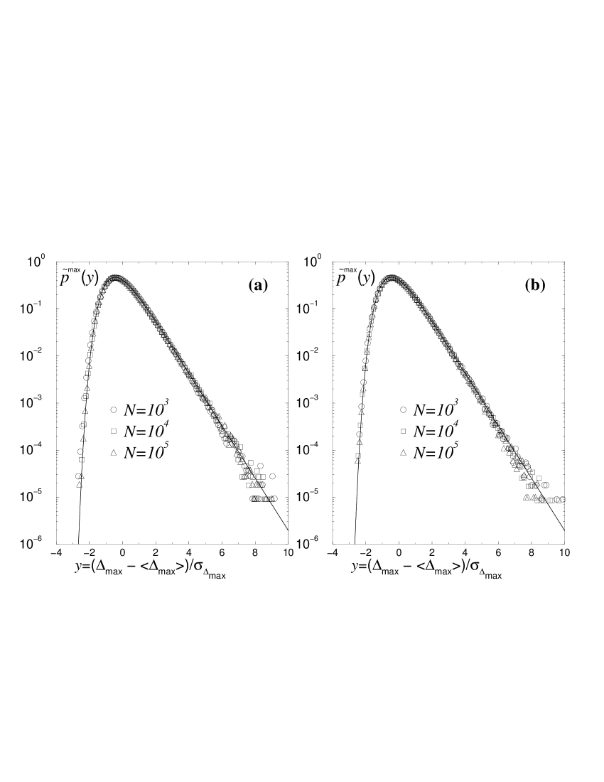
Figure 1: Disorder-averaged probability densities for the scaled (zero mean and unit variance) extreme-height fluctuations for the SW-synchronized PDES time horizons. (a) For the hard SW network with $p$$=$$0.10$ and (b) for the soft SW network with $p$$=$$0.50$, on log-normal scales for three system sizes. The solid curve corresponds to the similarly scaled FTG density note2 for comparison.

To study the extreme fluctuations of the SW-synchronized virtual time-horizon, we “simulated the simulations”, i.e., the evolution of the local simulated times based on the above exact algorithmic rules. By constructing histograms for $\Delta_{i}$, we observed that the tail of the disorder-averaged individual relative-height distribution decays exponentially for both SW constructions. Then, we constructed histograms for the scaled extreme-height fluctuations. The results, together with the similarly scaled FTG density note2 , are shown in Fig. 1. We also observed that the distribution of the extreme values becomes self-averaging, i.e., independent of the network realization. Finally, Fig. 2 shows that for sufficiently large $N$ (such that $w$ essentially becomes system-size independent) the average (or typical) size of the extreme-height fluctuations diverge logarithmically, according to Eq. (5) with $\delta$$=$$1$. We also found that the largest relative deviations below the mean $\langle\bar{h}$$-$$h_{\min}\rangle$, and the maximum spread $\langle h_{\max}$$-$$h_{\min}\rangle$ follow the same scaling with the system size $N$. Note, that for our specific system (PDES time horizon), the “microscopic” dynamics is inherently non-linear, but the effects of the non-linearities only give rise to a renormalized mass $\Sigma(p)$ (leaving $\Sigma(p)$$>$$0$ for all $p$$>$$0$) KORNISS03a ; future . Thus, the dynamics is effectively governed by relaxation in a small world, yielding a finite correlation length and, consequently, the slow logarithmic increase of the extreme fluctuations with the system size [Eq. (5)]. Also, for the PDES time horizon, the local height distribution is asymmetric with respect to the mean, but the average size of the height fluctuations is, of course, finite for both above and below the mean. This specific characteristic simply yields different prefactors for the extreme fluctuations [Eq. (5)] above and below the mean, leaving the logarithmic scaling with $N$ unchanged.

Figure 2: Average maximum relative height and average width for the SW-synchronized time horizon as a function of the number of nodes (PEs). Filled symbols: hard SW network with $p$$=$$0.10$. Open symbols: soft SW network with $p$$=$$0.50$. Note the normal-log scales.

In summary, we considered the extreme-height fluctuations in a prototypical model with local relaxation, unbounded local variables, and short-tailed noise. We argued, that when the interaction topology is extended to include random links in a SW fashion, the statistics of the extremes is governed by the FTG distribution. This finding directly addresses synchronizability in generic SW-coupled systems where relaxation through the links is the relevant node-to-node process and effectively governs the dynamics. We illustrated our results on an actual synchronizational problem in the context of scalable parallel simulations. Analogous questions for heavy-tailed noise distribution and different types of networks have relevance to various transport and transmission phenomena in natural and artificial networks flux . For example, heavy-tailed noise typically generates similarly tailed local field variables through the collective dynamics. Then, the largest fluctuations can still diverge as a power law with the system size (governed by the Fréchet distribution GUMBEL ; GALAMBOS ), motivating further research for the properties of extreme fluctuations in complex networks future .

We thank Z. Rácz, Z. Toroczkai, M.A. Novotny, and A. Middleton for comments and discussions. G.K. thanks CNLS LANL for their hospitality during Summer 2003. Supported by NSF Grant No. DMR-0113049 and the Research Corp. Grant No. RI0761. H.G. was also supported in part by the LANL summer student program in 2003 through US DOE Grant No. W-7405-ENG-36.

References

- (1) S.H. Strogatz, Nature 410, 268 (2001).
- (2) D.J. Watts and S.H. Strogatz, Nature 393, 440 (1998).
- (3) H. Hong, M.Y. Choi, and B.J. Kim, Phys. Rev. E 65, 047104 (2002).
- (4) G. Korniss, M.A. Novotny, H. Guclu, and Z. Toroczkai, P.A. Rikvold, Science 299, 677 (2003).
- (5) M.B. Hastings, Phys. Rev. Lett. 91, 098701 (2003).
- (6) B. Kozma, M.B. Hastings, and G. Korniss, arXiv:cond-mat/0309196 (2003).
- (7) R.A. Fisher and L.H.C. Tippett, Proc. Camb. Philos. Soc. 24, 180 (1928)
- (8) E.J. Gumbel, Statistics of Extremes (Columbia University Press, New York, 1958).
- (9) Extreme Value Theory and Applications, edited by J. Galambos, J. Lechner, and E. Simin (Kluwer, Dordrecht, 1994).
- (10) A.-L. Barabási and H.E. Stanley, Fractal Concepts in Surface Growth (Cambridge University Press, Cambridge, 1995).
- (11) S. Raychaudhuri, M. Cranston, C. Przybyla, and Y. Shapir, Phys. Rev. Lett. 87, 136101 (2001).
- (12) G. Korniss, M.A. Novotny, A.K. Kolakowska, and H. Guclu, SAC 2002, Proceedings of the 2002 ACM Symposium on Applied Computing, pp. 132-138, (2002).
- (13) R. Fujimoto, Commun. ACM 33, 30 (1990).
- (14) B.D. Lubachevsky, J. Comput. Phys. 75, 103 (1988).
- (15) G. Korniss, Z. Toroczkai, M.A. Novotny, and P.A. Rikvold, Phys. Rev. Lett. 84, 1351 (2000).
- (16) M. Kardar, G. Parisi, Y.-C. Zhang, Phys. Rev. Lett. 56, 889 (1986).
- (17) S.T. Bramwell, P.C.W. Holdsworth, and J.-F. Plinton, Nature 396 552 (1998).
- (18) S.T. Bramwell et al., Phys. Rev. Lett. 84, 3744 (2000).
- (19) V. Aji and N. Goldenfeld, Phys. Rev. Lett. 86, 1007 (2001).
- (20) T. Antal, M. Droz, G. Györgyi, and Z. Rácz, Phys. Rev. Lett. 87, 240601 (2001).
- (21) S. C. Chapman, G. Rowlands, and N. W. Watkins, Nonlinear Processes in Geophysics 9, 409 (2002).
- (22) J.-P. Bouchaud and M. Mézard, J. Phys. A 30, 7997 (1997).
- (23) A. Baldassarri, Statistics of Persistent Extreme Events, Ph.D. Thesis, De l´Université Paris XI Orsay (2000); http://axtnt3.phys.uniroma1.it/~andreab/these.html
- (24) Note that for , while the convergence to Eq. (2) is fast, the convergence for the appropriately scaled variable to the universal FTG distribution Eq. (3) is extremely slow FT ; AB .
- (25) S.F. Edwards and D.R. Wilkinson, Proc. R. Soc. London, Ser A 381, 17 (1982).
- (26) M.E.J. Newman, J. Stat. Phys. 101, 819 (2000).
- (27) M.E.J. Newman and D.J. Watts, Phys. Lett. A 263, 341 (1999).
- (28) R. Monasson, Eur. Phys. J. B 12, 555 (1999).
- (29) The exponent for the tail of the local relative height distribution may differ from that of the noise as a result of the collective (possibly non-linear) dynamics, but the exponential-like feature does not change.
- (30) When comparing with experimental or simulation data, instead of Eq. (3), it is often convenient to use the form of the FTG distribution which is scaled to zero mean and unit variance, yielding , where and is the Euler constant. The corresponding FTG density is then .
- (31) M. Argollo de Menezes and A-L. Barabási, arXiv:cond-mat/0306304 (2003).
- (32) H. Guclu and G. Korniss, to be published.