Electron transport through strongly interacting quantum dot coupled to normal metal and superconductor.

Abstract

We study the electron transport through the quantum dot coupled to the normal metal and $BCS$-like superconductor ($N-QD-S$) in the presence of the Kondo effect and Andreev scattering. The system is described by the single impurity Anderson model in the limit of strong on-dot interaction. We use recently proposed equation of motion technique for Keldysh nonequilibrium Green’s function together with the modified slave boson approach to study the electron transport. We derive formula for the current which contains various tunneling processes and apply it to study the transport through the system. We find that the Andreev conductance is strongly suppressed and there is no zero-bias (Kondo) anomaly in the differential conductance. We discuss effects of the particle-hole asymmetry in the electrodes as well as the asymmetry in the couplings.

1 Introduction

In recent years there has been much experimental and theoretical work on electron transport through nanometer-size areas (metallic or semiconducting islands) containing small number of electrons. These islands (sometimes called the quantum dots) are coupled via tunnel barriers to several external electrodes making it possible to adjust the current flowing through the system [1]. The devices give a new possibility of studying several well-known quantum phenomena in novel and highly controllable way. For instance, it is well known, that quantum dot behaves like magnetic impurity in a metallic host and in particular displays the Kondo effect [2]-[5]. Kondo effect is a manifestation of the simplest state formed by the impurity spin and conduction electron spins. This state gives rise to a quasiparticle peak at the Fermi energy in the dot spectral function [6]-[9] and zero-bias maximum in the differential conductance observed experimentally [10]-[14].

Another example is the Andreev scattering [15], according to which an electron impinging on normal metal - superconductor interface is reflected back as a hole and the Cooper pair is created in superconductor. This effect has been shown to play crucial role in the transport properties of various hybrid mesoscopic superconducting devices [16]. There is a number of papers in the literature concerning the electron transport in various realizations of such devices. Here we are interested in study of the normal state quantum dot coupled to one normal and one superconducting electrode ($N-QD-S$). Such system was studied within scattering matrix technique [17, 18]. However this approach is valid only for noninteracting systems and cannot take into account effects of Coulomb interactions between electrons on the dot, which are very important in these small systems, as they lead e.g. to the Coulomb blockade phenomena [19] or Kondo effect [2]-[5]. Transport through noninteracting quantum dot has also been studied within nonequilibrium Green’s function technique. The effect of multiple discrete levels of the dot was discussed in Refs.[20, 21], the photon-assistant transport in [22], electron transport in the weak magnetic field in [23], temperature dependence of the resonant Andreev reflections in [24] and transport in three terminal system (two ferromagnetic and one superconducting electrodes) in [25].

In the presence of strong Coulomb interaction in $N-QD-N$ device the Kondo effect appears an influences the electron transport in the system. If one of the electrodes is superconducting both single electron and the Andreev current is affected by the Abrikosov - Suhl resonance. This problem has been extensively studied within various techniques [21, 26]-[33] and there is no consensus. Some authors have predicted suppression [21, 26, 30, 31] of the conductance due to Andreev reflections while others - enhancement [27, 29]. Recently it has been shown [32] that one can obtain either suppression or enhancement of the conductance in dependence on the values of the model parameters. Recently other effects like emergence of the Kondo-like peaks in the local density of states ($DOS$) at energies equal to $\pm\Delta$ ($\Delta$ is the superconducting order parameter) [30, 32] or a novel co-tunneling process (Andreev-normal co-tunneling) [33] have been revealed. This process involves Andreev tunneling from the $QD-S$ interface and normal tunneling from $N-QD$ interface. As a result the Cooper pair directly participates in the formation of the spin singlet (Kondo effect) and leads to emergence of the additional Kondo resonances in the local $DOS$ and enhancement of the tunneling current.

The purpose of the present work is to apply the new technique to derive formula for the current through $QD$ (in the limit of strong on-dot Coulomb interaction) in terms of various tunneling processes. We also study the interplay between the Kondo effect and Andreev reflections to give additional insight into the the problem of the suppression/enhancement of the zero-bias current-voltage anomaly. Further we discuss the question of participation of the superconducting electrons in creation of the Kondo effect. And finally we investigate the influence of the electron - hole asymmetry in the leads on tunneling transport as well as the asymmetry in the couplings to the leads.

The paper is organized as follows. In section 2 we present model under consideration and derive formula for the current using $EOM$ for nonequilibrium $GF$. In section 3 we apply the obtained formula for the current to the numerical study of the transport through $N-QD-S$ system. Section 4 is devoted to the interplay between the Kondo and Andreev scattering. In section 5 we discuss the quantum dot asymmetrically coupled to the leads, while the effect of electron - hole asymmetry in the leads is investigated in sec. 6. Some conclusions are given in sec. 7.

2 Model and formulation

The Anderson Hamiltonian of the single impurity [34], in the Nambu representation, can be written in the form

$$H=\sum_{\lambda{\bf k}\sigma}\Psi^{+}_{\lambda{\bf k}\sigma}H^{0}_{\lambda{\bf k}}\Psi_{\lambda{\bf k}\sigma}+$$

$$\sum_{\sigma}\Phi^{+}_{\sigma}H^{QD}\Phi_{\sigma}+\sum_{\lambda{\bf k}\sigma}\Psi^{+}_{\lambda{\bf k}\sigma}H^{I}_{\lambda{\bf k}}\Phi_{\sigma}$$ (1)

where the Nambu spinors $\Psi_{\lambda{\bf k}\sigma}$ and $\Phi_{\sigma}$ are defined as

$$\Psi_{\lambda{\bf k}\sigma}=\left(\begin{array}[]{l}c_{\lambda{\bf k}\sigma}\\ c^{+}_{\lambda{-\bf k}-\sigma}\end{array}\right)\;\;\;\;\;\;;\;\;\;\;\;\;\Phi_{\sigma}=\left(\begin{array}[]{l}d_{\sigma}\\ d^{+}_{-\sigma}\end{array}\right)$$ (6)

and

$$H^{0}_{\lambda{\bf k}}=\left(\begin{array}[]{cr}\epsilon_{\lambda{\bf k}}&\Delta_{\lambda{\bf k}}\\ \Delta^{*}_{\lambda{\bf k}}&-\epsilon_{\lambda{\bf k}}\end{array}\right)$$ (9)

denotes Hamiltonian of the normal ($\Delta_{N{\bf k}}=0$) or superconducting ($\Delta_{S{\bf k}}\neq 0$) lead.

$$H^{QD}=\left(\begin{array}[]{cc}E_{d}+U_{d}n_{-\sigma}&0\\ 0&-(E_{d}+U_{d}n_{\sigma})\end{array}\right)$$ (12)

is the dot Hamiltonian and

$$H^{I}_{\lambda{\bf k}}=\left(\begin{array}[]{cr}V_{\lambda{\bf k}}&0\\ 0&-V_{\lambda{\bf k}}\end{array}\right)$$ (15)

the dot-electrode hybridization. Here $\lambda=N$, $S$ denotes the normal metal ($N$) or superconducting ($S$) lead in the system. The parameters have the following meaning: $c^{+}_{\lambda{\bf k}\sigma}$ ($c_{\lambda{\bf k}\sigma}$) denotes creation (annihilation) operator for a conduction electron with the wave vector ${\bf k}$, spin $\sigma$ in the lead $\lambda$, $\Delta_{\lambda{\bf k}}$ is the superconducting order parameter in the lead $\lambda$ ($\Delta_{S{\bf k}}=\Delta_{S}$, $\Delta_{N{\bf k}}=0$) , and $V_{\lambda{\bf k}}$ is the hybridization matrix element between conduction electron of energy $\epsilon_{\lambda{\bf k}}$ in the lead $\lambda$ and localized electron on the dot with the energy $E_{d}$. $d^{+}_{\sigma}$ ($d_{\sigma}$) is the creation (annihilation) operator for an electron on the dot and $U_{d}$ is the on-dot Coulomb repulsion.

To derive the formula for the average current in the system we start from the time derivative of the charge (for convenience we perform calculations in the normal electrode) [36]:

$$J=-e\frac{d}{dt}\langle N_{N}\rangle=\frac{ie}{\hbar}\langle[N_{N},H]_{-}\rangle$$ (16)

, where $N_{N}=\sum_{{\bf k}\sigma}c^{+}_{N{\bf k}\sigma}c_{{\bf k}\sigma}$ is the total electron number operator in the lead $N$ and $e$ is the elementary charge. The above formula can be written in terms of the Green’s functions ($GF$):

$$J=-\frac{2e}{\hbar}\sum_{{\bf k}\sigma}\int^{\infty}_{-\infty}\frac{d\omega}{2\pi}[H^{I}_{N{\bf k}}G^{<}_{N{\bf k}\sigma,d}(\omega)]_{11}$$ (17)

, where $G^{<}_{N{\bf k},d\sigma}(\omega)$ is the Fourier transform of the Keldysh matrix Green’s function [35] $G^{<}_{N{\bf k},d\sigma}(t)=i\langle\Phi^{+}_{\sigma}(0)\otimes\Psi_{N{\bf k}\sigma}(t)\rangle$. Now we have to calculate the Green’s function $G^{<}_{N{\bf k},d\sigma}(\omega)$. One can do this in the usual way, i. e.. using Keldysh equation [35, 36]

$$G^{<}(\omega)=(1+G^{r}(\omega)\Sigma^{r}(\omega))G^{<}_{0}(\omega)$$

$$\times(1+\Sigma^{a}(\omega)G^{a}(\omega))+G^{r}(\omega)\Sigma^{<}(\omega)G^{a}(\omega)$$ (18)

(superscripts $r,a$ are for retarded and advanced $GF$ respectively) and make more or less justified approximations for the ’lesser’ self-energy $\Sigma^{<}(\omega)$. Usually one uses approximation due to Ng [37] which states that full ’lesser’ self-energy is proportional to the noninteracting one ($\Sigma^{<}(\omega)\propto\Sigma^{<}_{0}(\omega)$). This approximation is widely used in the literature [26, 28]. However we wish to use another approach based on recently proposed equation of motion technique ($EOM$) for nonequilibrium Green’s functions [38]. The usual equation of motion derived from Heisenberg equation yields undefined singularities, which depend on the initial conditions. The advantage of this new technique, based on Schwinger - Keldysh perturbation formalism, is that it explicitly determine these singular terms. Moreover, together with $EOM$ for retarded (advanced) Green’s functions it allows to treat the problem in very consistent way making similar approximations in the decoupling procedure for all types of the Green’s functions. Such approach was recently proposed to calculate the charge on the quantum dot upon nonequilibrium conditions [39].

According to the Ref.[38] the equation for the ’lesser’ Green’s functions reads:

$$\langle\langle A|B\rangle\rangle^{<}_{\omega}=g^{<}(\omega)\langle[A,B]_{\pm}\rangle+$$

$$g^{r}(\omega)\langle\langle[A,H_{I}]_{-}|B\rangle\rangle^{<}_{\omega}+g^{<}(\omega)\langle\langle[A,H_{I}]_{-}|B\rangle\rangle^{a}_{\omega}$$ (19)

where $g^{r(<)}(\omega)$ is the free electron $GF$ and $H_{I}$ denotes interacting part of the Hamiltonian. In general this equation allows to calculate the the $GF$ on the left hand side, however in practice we have to approximate the higher order $GF$-s appearing on the right hand side (as in $EOM$ for equilibrium $GF$-s). But performing analogous approximations in the decoupling procedure for both retarded and ’lesser’ $GF$ we make theory consistent.

Applying above equation for the Green’s function occurring in the formula for the current (17) $G^{<}_{N{\bf k}\sigma,d}(\omega)$, we get following expression:

$$\langle\langle\Psi_{N{\bf k}\sigma}|\Phi^{+}_{\sigma}\rangle\rangle^{<}_{\omega}=g^{r}_{N{\bf k}}(\omega)H^{I}_{N{\bf k}}\langle\langle\Phi_{\sigma}|\Phi^{+}_{\sigma}\rangle\rangle^{<}_{\omega}+$$

$$g^{<}_{N{\bf k}}(\omega)H^{I}_{N{\bf k}}\langle\langle\Phi_{\sigma}|\Phi^{+}_{\sigma}\rangle\rangle^{a}_{\omega}$$ (20)

where as an interacting part of Hamiltonian $H_{I}$ we have taken the third term in the Eq.(1). $g^{r(<)}_{N{\bf k}}(\omega)$ is retarded (’lesser’) free-electron matrix $GF$ of the normal-state electrode.

$$g^{r}_{N{\bf k}}(\omega)=\left(\begin{array}[]{cc}\frac{1}{\omega-\epsilon_{N{\bf k}}+i0}&0\\ 0&\frac{1}{\omega+\epsilon_{N{\bf k}}+i0}\end{array}\right)$$ (23)

$$g^{<}_{N{\bf k}}(\omega)=\left(\begin{array}[]{cc}2\pi if(\omega-eV)\delta(\omega-\epsilon_{N{\bf k}})&0\\ 0&2\pi if(\omega+eV)\delta(\omega+\epsilon_{N{\bf k}})\end{array}\right)$$ (26)

where $f(\omega)$ is the Fermi distribution function and $eV=\mu_{N}-\mu_{S}$ corresponds to the applied voltage between normal state electrode with the chemical potential $\mu_{N}$ and superconducting one with $\mu_{S}$. In the following we fix the chemical potential of the $SC$ electrode ($\mu_{S}=0$) and use $eV$ as a measure of the bias voltage.

Expression (20) is general for Anderson model and doesn’t depend explicitly on the form of the Hamiltonian describing quantum dot ($H_{QD}$). The dependence enters only through the Green’s function $G^{<(a)}_{d\sigma}(\omega)=\langle\langle\Phi_{\sigma}|\Phi^{+}_{\sigma}\rangle\rangle^{<(a)}_{\omega}$. In the following we wish to study quantum dot in the limit of strong on-dot Coulomb repulsion ($U_{d}\rightarrow\infty$). In this limit double occupancy of the dot is forbidden and it is convenient to work in the slave boson representation in which the real electron operator is replaced by product of fermion and boson ones ($d_{\sigma}\Rightarrow b^{+}f_{\sigma}$) [40, 41]. Additionally the fact that there is no double occupancy on the dot should be taken into account in some way. Usually such constraint is added to the Hamiltonian by the Lagrange multiplier. There is a number of variants of this approach in the literature and here we shall work within La Guillou - Ragoucy scheme [42, 43]. In this approach the constraint of no double occupancy is enforced through modification of the commutation relations of both fermion and boson operators in comparison to the standard ones. This approach was successfully used in the study of the charge on the quantum dot [39].

Hamiltonian of the system in the limit $U_{d}\rightarrow\infty$ in the slave boson representation is given in the form (1), but now with

$$\Phi_{\sigma}=\left(\begin{array}[]{l}b^{+}f_{\sigma}\\ f^{+}_{-\sigma}b\end{array}\right)$$ (29)

and

$$H^{QD}=\left(\begin{array}[]{cc}E_{d}&0\\ 0&-E_{d}\end{array}\right)$$ (32)

Having introduced slave boson representation, we can begin calculations of the advanced and ’lesser’ on-dot $GF$s appearing in Eq. (20). To do this we apply formula (19) together with usual prescription for the advanced (retarded) $GF$. One can investigate that on the higher-order $GF$s appeared in the this process have similar form in both cases: ’lesser’ and advanced. So idea is to make the same approximations in the procedure of decoupling of the higher order $GF$s. Explicitly, we have performed decoupling

$$\langle\langle c^{+}_{\lambda{\bf k}\sigma}c_{\lambda^{\prime}{\bf k}^{\prime}\sigma}A|B\rangle\rangle_{\omega}\approx\delta_{\lambda\lambda^{\prime}}\delta_{{\bf kk}^{\prime}}n_{\lambda{\bf k}}\langle\langle A|B\rangle\rangle_{\omega}$$ (33)

and neglected the other $GF$s. In above formula $n_{\lambda{\bf k}}$ is the concentration of the electrons in the lead $\lambda$ in state ${\bf k}$ and for superconducting electrode is given by

$$n_{S{\bf k}}=\frac{1}{2}\left[1-\frac{\epsilon_{S{\bf k}}}{E_{S{\bf k}}}\left(1-2f(E_{S{\bf k}})\right)\right]$$ (34)

with quasiparticle spectrum $E^{2}_{S{\bf k}}=\epsilon^{2}_{S{\bf k}}+\Delta^{2}_{S}$, while for the normal lead this relation reduces to

$$n_{N{\bf k}}=f(\epsilon_{N{\bf k}}-eV)$$ (35)

We want to stress here, that we haven’t used factorization like

$$\langle\langle c^{+}_{\lambda{\bf k}\sigma}c^{+}_{\lambda^{\prime}{\bf k}^{\prime}\sigma}A|B\rangle\rangle_{\omega}\approx\delta_{\lambda\lambda^{\prime}}\delta_{{\bf k}-{\bf k}^{\prime}}\langle c^{+}_{\lambda{\bf k}\sigma}c^{+}_{\lambda-{\bf k}\sigma}\rangle\langle\langle A|B\rangle\rangle_{\omega}$$ (36)

The reason comes from the requirement of the hermicity relation between retarded and advanced Green’s function, i. e.. $G^{r}(\omega)=[G^{a}(\omega)]^{\dagger}$. If we calculate retarded $GF$ within $EOM$ and perform the same decoupling as in advanced Green’s function keeping also $\langle c^{+}_{\lambda{\bf k}\sigma}c^{+}_{\lambda-{\bf k}\sigma}\rangle$ terms, we get expressions for the $GF$s which violates the hermicity relation. The only way to fulfill that at this level is to make approximations due to (33) and neglect the remaining higher order $GF$s.

The resulting advanced on-dot $GF$ $G^{a}_{d\sigma}(\omega)$ can be written in the form of the Dyson equation:

$$G^{a}_{d\sigma}(\omega)=g^{a}_{d\sigma}(\omega)+g^{a}_{d\sigma}(\omega)\Sigma^{a}_{d\sigma}(\omega)G^{a}_{d\sigma}(\omega)$$ (37)

where $g^{a}_{d\sigma}(\omega)$ non-perturbed dot’s advanced Green’s function:

$$g^{a}_{d\sigma}(\omega)=\left(\begin{array}[]{cc}\frac{1-n_{-\sigma}}{\omega-E_{d}-i0}&0\\ 0&\frac{1-n_{\sigma}}{\omega+E_{d}-i0}\end{array}\right)$$ (40)

and self energy $\Sigma^{a}_{d\sigma}(\omega)$ which can be written as sum of the noninteracting $\Sigma^{0a}_{d}(\omega)$ and interacting $\Sigma^{Ia}_{d}(\omega)$ part

$$\Sigma^{a}_{d}(\omega)=\Sigma^{0a}_{d}(\omega)+\Sigma^{Ia}_{d}(\omega)=\sum_{\lambda{\bf k}}\left[\Sigma^{0a}_{\lambda{\bf k}}(\omega)+\Sigma^{Ia}_{\lambda{\bf k}}(\omega)\right]$$ (41)

For superconducting electrode we have

$$\Sigma^{0a}_{S{\bf k}}(\omega)=\left(\begin{array}[]{cc}\frac{|V_{S{\bf k}}|^{2}}{(1-n_{-\sigma})}\left(\frac{u^{2}_{S{\bf k}}}{\omega-E_{S{\bf k}}-i0}+\frac{v^{2}_{S{\bf k}}}{\omega+E_{S{\bf k}}-i0}\right)&\frac{|V_{S{\bf k}}|^{2}}{(1-n_{\sigma})}\left(\frac{u_{S{\bf k}}v_{S{\bf k}}}{\omega+E_{S{\bf k}}-i0}-\frac{u_{S{\bf k}}v_{S{\bf k}}}{\omega-E_{S{\bf k}}-i0}\right)\\ \\ \frac{|V_{S{\bf k}}|^{2}}{(1-n_{-\sigma})}\left(\frac{u_{S{\bf k}}v_{S{\bf k}}}{\omega+E_{S{\bf k}}-i0}-\frac{u_{S{\bf k}}v_{S{\bf k}}}{\omega-E_{S{\bf k}}-i0}\right)&\frac{|V_{S{\bf k}}|^{2}}{(1-n_{\sigma})}\left(\frac{v^{2}_{S{\bf k}}}{\omega-E_{S{\bf k}}-i0}+\frac{u^{2}_{S{\bf k}}}{\omega+E_{S{\bf k}}-i0}\right)\\ \end{array}\right)$$ (45)

where we have introduced $BCS$ factors $u^{2}_{S{\bf k}}=\frac{1}{2}\left(1+\frac{\epsilon_{S{\bf k}}}{E_{S{\bf k}}}\right)$, $v^{2}_{S{\bf k}}=\frac{1}{2}\left(1-\frac{\epsilon_{S{\bf k}}}{E_{S{\bf k}}}\right)$. For the normal state corresponding expression is:

$$\Sigma^{0a}_{N{\bf k}}(\omega)=\left(\begin{array}[]{cc}\frac{|V_{N{\bf k}}|^{2}}{(1-n_{-\sigma})}\frac{1}{\omega-\epsilon_{N{\bf k}}-i0}&0\\ 0&\frac{|V_{N{\bf k}}|^{2}}{(1-n_{\sigma})}\frac{1}{\omega+\epsilon_{N{\bf k}}-i0}\\ \end{array}\right)$$ (48)

It turns out that within the present approach the interacting part of the self energy is simply related to the noninteracting one. Moreover the same relation also holds for retarded as well as ’lesser’ $GF$s. This is a result of the consistency of the decoupling procedure and requirement of the hermicity relation between retarded and advanced $GF$. In general this relation can be written as:

$$\Sigma^{I}_{\lambda{\bf k}}(\omega)=n_{\lambda{\bf k}}\tau_{3}\Sigma^{0}_{\lambda{\bf k}}(\omega)\tau_{3}$$ (49)

where $\tau_{3}=\left(\begin{array}[]{cr}1&0\\ 0&-1\\ \end{array}\right)$ is the Pauli matrix and $n_{\lambda{\bf k}}$ is the concentration of the electrons of the wave vector ${\bf k}$ in the lead $\lambda$ given by (34) and (35).

It is possible to write Eq. for the ’lesser’ $GF$ in the form of the Keldysh equation (18) with $G^{a}_{d\sigma}(\omega)$ given by Eq.(37) and $G^{r}=[G^{a}]^{\dagger}$. Free electron dot’s ’lesser’ Green’s function is given in the form:

$$g^{<}_{d\sigma}(\omega)=\left(\begin{array}[]{cc}2\pi i(1-n_{-\sigma})f(\omega)\delta^{-}_{d}&0\\ 0&2\pi i(1-n_{\sigma})f(\omega)\delta^{+}_{d}\end{array}\right)$$ (52)

where $\delta^{\pm}_{d}=\delta(\omega\pm E_{d})$. As we have mentioned, the ’lesser’ self energy has the same form as advanced one:

$$\Sigma^{<}_{d}(\omega)=\Sigma^{0<}_{d}(\omega)+\Sigma^{I<}_{d}(\omega)=\sum_{\lambda}(\Sigma^{0<}_{\lambda{\bf k}}(\omega)+\Sigma^{I<}_{\lambda{\bf k}}(\omega))$$ (53)

where noninteracting part due to $SC$ lead is:

$$\Sigma^{0<}_{S{\bf k}}(\omega)=2\pi if(\omega)\left(\begin{array}[]{cc}\frac{|V_{S{\bf k}}|^{2}}{(1-n_{-\sigma})}\left(u^{2}_{S{\bf k}}\delta^{-}_{S}+v^{2}_{S{\bf k}}\delta^{+}_{S}\right)&\frac{|V_{S{\bf k}}|^{2}}{(1-n_{\sigma})}u_{S{\bf k}}v_{S{\bf k}}\left(\delta^{+}_{S}-\delta^{-}_{S}\right)\\ \\ \frac{|V_{S{\bf k}}|^{2}}{(1-n_{-\sigma})}u_{S{\bf k}}v_{S{\bf k}}\left(\delta^{+}_{S}-\delta^{-}_{S}\right)&\frac{|V_{S{\bf k}}|^{2}}{(1-n_{\sigma})}\left(v^{2}_{S{\bf k}}\delta^{-}_{S}+u^{2}_{S{\bf k}}\delta^{+}_{S}\right)\\ \end{array}\right)$$ (57)

and for the normal lead we have

$$\Sigma^{0<}_{N{\bf k}}(\omega)=2\pi i\left(\begin{array}[]{cc}\frac{|V_{N{\bf k}}|^{2}}{(1-n_{-\sigma})}f(\omega-eV)\delta^{-}_{N}&0\\ 0&\frac{|V_{N{\bf k}}|^{2}}{(1-n_{\sigma})}f(\omega+eV)\delta^{+}_{N}\\ \end{array}\right)$$ (60)

where $\delta^{\pm}_{S}=\delta(\omega\pm E_{S{\bf k}})$ and $\delta^{\pm}_{N}=\delta(\omega\pm\epsilon_{N{\bf k}})$. And again, the interacting part of the ’lesser’ self energy is related to the noninteracting one simply through Eq.(49).

Now we are ready to write the expression for the current (17) in terms of known $GF$s. First, let’s rewrite the Keldysh equation for the element $11$ of the dot’s $GF$ in the form:

$$G^{<}_{11}=G^{r}_{11}\Sigma^{<}_{11}G^{a}_{11}+G^{r}_{11}\Sigma^{<}_{12}G^{a}_{21}+$$

$$G^{r}_{12}\Sigma^{<}_{21}G^{a}_{11}+G^{r}_{12}\Sigma^{<}_{22}G^{a}_{21}$$ (61)

Note that we don’t have term proportional to $g^{<}_{d}$ as it vanishes in our case [36].

To calculate the $GF$ given by Eq.(20), entering to the expression for the current (17), we need yet element $11$ of the advanced $GF$, more precisely imaginary part of that. Note that $g^{<}_{N{bfk}}$ is purely imaginary and we need real part of $g^{<}_{N{\bf k}}G^{a}_{d}$. We can write down equation for the imaginary part of the element $11$ of $G^{a}_{d}$ in the similar fashion as Eq.(61), i.e.

$${\it Im}G^{a}_{11}=G^{r}_{11}{\it Im}\Sigma^{a}_{11}G^{a}_{11}+G^{r}_{11}{\it Im}\Sigma^{a}_{12}G^{a}_{21}+$$

$$G^{r}_{12}{\it Im}\Sigma^{a}_{21}G^{a}_{11}+G^{r}_{12}{\it Im}\Sigma^{a}_{22}G^{a}_{21}$$ (62)

Substituting now the Eqs. (61) and (62) into (20) we get expression for the $G_{N{\bf k},d}$, which determines the current (17). Finally the current (17) can be written as

$$J=J_{11}+J_{22}+J_{12}+J_{A}$$ (63)

The first term represents conventional tunneling and is given in the form

$$J_{11}=-\frac{2e}{\hbar}\int^{\infty}_{-\infty}\frac{d\omega}{2\pi}{\it Im}\Sigma^{S}_{11}|G_{11}|^{2}$$

$$\Gamma_{N}\rho^{N}_{11}[f(\omega-eV)-f(\omega)]$$ (64)

where is the elastic rate defined as $\Gamma_{N}=2\pi V^{2}_{N}\rho^{N}(0)$ and $\rho^{N}(0)$ is the bare normal state density of states at the Fermi energy. The second term describes the ’branch crossing’ process (process with crossing through the Fermi surface) in the language of the $BTK$ theory (Blonder - Tinkham - Klapwijk) [44]: electron from the normal lead is converted into the hole like in the $SC$ lead.

$$J_{22}=-\frac{2e}{\hbar}\int^{\infty}_{-\infty}\frac{d\omega}{2\pi}{\it Im}\Sigma^{S}_{22}|G_{12}|^{2}$$

$$\Gamma_{N}\rho^{N}_{11}[f(\omega-eV)-f(\omega)]$$ (65)

The next term corresponds to the process in which electron tunnels into $SC$ picking up the quasiparticle and creating a Cooper pair.

$$J_{12}=-\frac{4e}{\hbar}\int^{\infty}_{-\infty}\frac{d\omega}{2\pi}{\it Im}\Sigma^{S}_{12}{\it Re}[G_{11}G^{*}_{12}]$$

$$\Gamma_{N}\rho^{N}_{11}[f(\omega-eV)-f(\omega)]$$ (66)

The last term in (63) represents Andreev tunneling in which electron from the normal lead is reflected back as a hole and Cooper pair is created in superconducting electrode.

$$J_{A}=-\frac{2e}{\hbar}\int^{\infty}_{-\infty}\frac{d\omega}{2\pi}{\it Im}\Sigma^{N}_{22}|G_{12}|^{2}$$

$$\Gamma_{N}\rho^{N}_{11}[f(\omega-eV)-f(\omega+eV)]$$ (67)

As one can see, at energies $|eV|<\Delta_{S}$ and zero temperature, the only process which contribute to the total current, is the Andreev tunneling. The remaining ones represent ’single particle’ processes which are suppressed at $|eV|<\Delta_{S}$ due to the lack of the states in superconductor. Of course for energies $|eV|>\Delta_{S}$ all these processes give rise to the current, even Andreev does, however is strongly suppressed, but still finite. It is also worthwhile to note that all these processes (except $J_{11}$) proceed through virtual states on the dot.

3 Density of states

In the following sections we will present numerical results of electron tunneling in the $N-QD-S$ system and show how different terms of Eq. (63) contribute to the total current and differential conductance. But firstly we want to turn our attention to the density of states as it gives a lot of information about system.

The most pronounced fingerprint of the Kondo effect in the $N-QDN$ system is the Abrikosov - Suhl or Kondo resonance at the Fermi level and its temperature dependence. Kondo resonance appears as temperature is lower than parameter dependent Kondo temperature $T_{K}$. In the original Kondo effect there is odd number of electrons on the dot, so the total spin is half - integer. In this case electrons from the leads with energy close to Fermi level screen the spin on the dot producing resonance at the Fermi energy. If electrodes are made superconducting situation is more complicated, as there enters another energy scale - superconducting transition temperature $T_{c}$ (or equivalently $SC$ order parameter $\Delta$). And the Kondo effect takes place provided $T_{K}>T_{c}$, otherwise is absent due to lack of the low energy states in the leads to screen the spin on the dot. Naturally there raises a question what will happen if one of the lead is superconducting and another in the normal state. This was investigated in [26]-[28], [30] and it has been found that Kondo effect survives in the presence of superconductivity in one of the electrodes, even $T_{K}<T_{c}$. The reason for this is simply: the spin of the dot is screened by electrons in the normal lead. We will show that this is a really the case and this is seen in the density of states of quantum dot.

In the Fig.1 we show the density of states of the quantum dot for various positions of the dot energy level $E_{d}$.

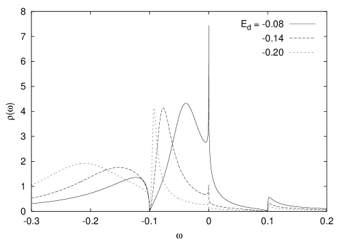
Figure 1: The density of states of the quantum dot for various values of the dot energy level $E_{d}$. Other parameters are following: $\Gamma_{N}=\Gamma_{S}=0.02$, $\Delta=0.1$, $eV=0$, $T=10^{-5}$ in the units of the bandwidth $W$.

It is clearly seen that Kondo effect, which manifests itself in the resonance on the Fermi level, survives the presence of superconductivity in one electrode. The additional structure at $\omega=\pm\Delta$ coming from the $SC$ lead is also visible. This is simply reflection of the $SC$ gap. At this point it worthwhile to note, that if $|E_{d}|>\Delta$ there is bound-like (Andreev) state within the $SC$ gap, position of which depends on $E_{d}$. In the $S-QD-S$ system this is a true bound state. However in the present case, due to finite $DOS$ in the normal lead, this state acquires a finite width (resonance state).

It is very interesting to see how the $DOS$ will be look like in the nonequilibrium situation ($eV=\mu_{N}-\mu_{S}=\neq 0$). Let us recall that the Kondo resonance is located at the Fermi level of the lead. In the $N-QD-N$ system when $eV\neq 0$ there emerge two resonances at Fermi levels of the left and right lead respectively. In our case there is a gap in the $SC$ lead $DOS$, and if our simple picture that Kondo effect is only due to normal lead, we expect only one resonance pinned to the normal metal electrode Fermi level ($\mu_{N}$). As we can learn from the Fig.2 this is really the case - the Kondo resonance follows the Fermi level of the normal lead.

Figure 2: Equilibrium ($eV=0$) and nonequilibrium ($eV=\pm 0.01$) density of states of the quantum dot. Other parameters have following values: $\Gamma_{N}=\Gamma_{S}=0.02$, $\Delta=0.1$, $E_{d}=-0.08$, $T=10^{-5}$ in units of the bandwidth $W$.

In the Fig.3 the $DOS$ is plotted for a few values of the $SC$ order parameter $\Delta$.

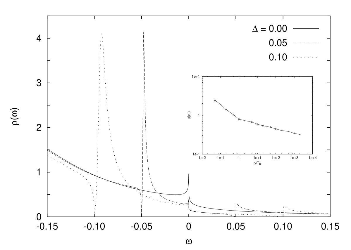
Figure 3: Equilibrium density of states of the quantum dot for various values of the order parameter ($\Delta$). $E_{d}=-0.2$ and other parameters have values as in the Fig.(2).

As we can see the Kondo resonance is strongly suppressed in comparison to the $N-QD-N$ $DOS$ (solid line). The reason for that is that due to lack of the low laying states in $SC$, the spin on the dot is weakly screened. Similar conclusions have been reached by A. A. Clerk and coworkers [30] within $NCA$ approach. In the inset the density of states at the Fermi level $\rho(\varepsilon_{F})$ is plotted as a function of the $SC$ order parameter $\Delta$.

Finally we want to discuss the temperature dependence of the dot density of states. In the Fig.4 we show the $DOS$ for number of temperatures.

Figure 4: Temperature dependence of the $DOS$ for $\Gamma_{N}=0.05$, $\Gamma_{S}=0.02$, $\Delta=0.05$, $E_{d}=-0.2$, $eV=0$.

As we expected the Kondo resonance disappears as temperature is raised. However it is important to stress out that resonances and dips $\omega\approx\Delta$ are also temperature dependent. It is clearly seen in the Fig.5, where height of the peaks $(a)$ and dips $(b)$ are shown.

Figure 5: Temperature dependence of height of the peaks $(a)$ and dips $(b$) near $\pm\Delta$ (see Fig.(3)). For comparison the temperature dependence of the Kondo resonance is also shown. The parameters are the same as in the Fig(3).

The spectral weight of the Kondo resonance is also shown for comparison. It is worthwhile to note that below $T_{K}$ the height of both peaks and dips are constant. As soon as temperature exceeds $T_{K}$ height of these resonances starts to raise as well as dips does. This effect can be though of as a transfer of the spectral weight between Kondo resonance and Andreev states. Let us remind that Andreev processes still take place at $T>T_{K}$ but less than $T_{c}$. We want to notice that our results are in contradiction to what has been found in Ref.[30] within $NCA$. The authors of [30] have shown that the resonances at $\pm\Delta$ do not appear at higher temperatures. This has a important consequences. This means that, even for $T_{c}>T_{K}$, superconducting electrons do participate in the Kondo effect. So our simple picture breaks down.

As we mentioned, they applied $NCA$ technique to calculate the dot $DOS$, which is known to give correct results in the normal state for a wide range of temperatures. It is also known, that $EOM$ gives quantitatively incorrect results at low temperatures ($T<T_{K}$). But here this effect certainly take place at $T>T_{K}$ in the range of validity of $EOM$. So the question of which picture is indeed realized in the real system seems to remain open.

4 Andreev reflections and the Kondo effect

We have shown, that Kondo peak in the density of states survives the presence of the superconductivity, however should we expect that peak in the current - voltage characteristic (differential conductance - $G(eV)=dJ/d(eV)$) ? If we consider tunneling processes, described by Eqs. (63)-(67), we might expect Kondo peak only in the tunneling mediated by the Andreev reflections (67). The amplitudes of the other processes is equal to zero (at $T=0$) for energies less than $SC$ gap.

Let’s rewrite Eq. (67) into the form:

$$J_{A}=-\frac{2e}{h}\int^{\infty}_{-\infty}\frac{d\omega}{2\pi}T^{A}_{NS}(\omega)[f(\omega-eV)-f(\omega+eV)]$$ (68)

We have introduced ’transmittance’ $T^{A}_{NS}(\omega)$, associated with the Andreev tunneling, defined as:

$$T^{A}_{NS}(\omega)=\frac{e}{\hbar}\Gamma^{2}_{N}\rho^{N}_{11}(\omega)\rho^{N}_{22}(\omega)|G_{21}(\omega)|^{2}$$ (69)

In fact, at zero temperature and at energies less than superconducting gap $T^{A}_{NS}(\omega)$ can be regarded as a total transmittance, because Andreev tunneling is only process allowed in these circumstances. $T^{A}_{NS}(\omega)$ for different values of the $eV$ is plotted in the Fig. 6.

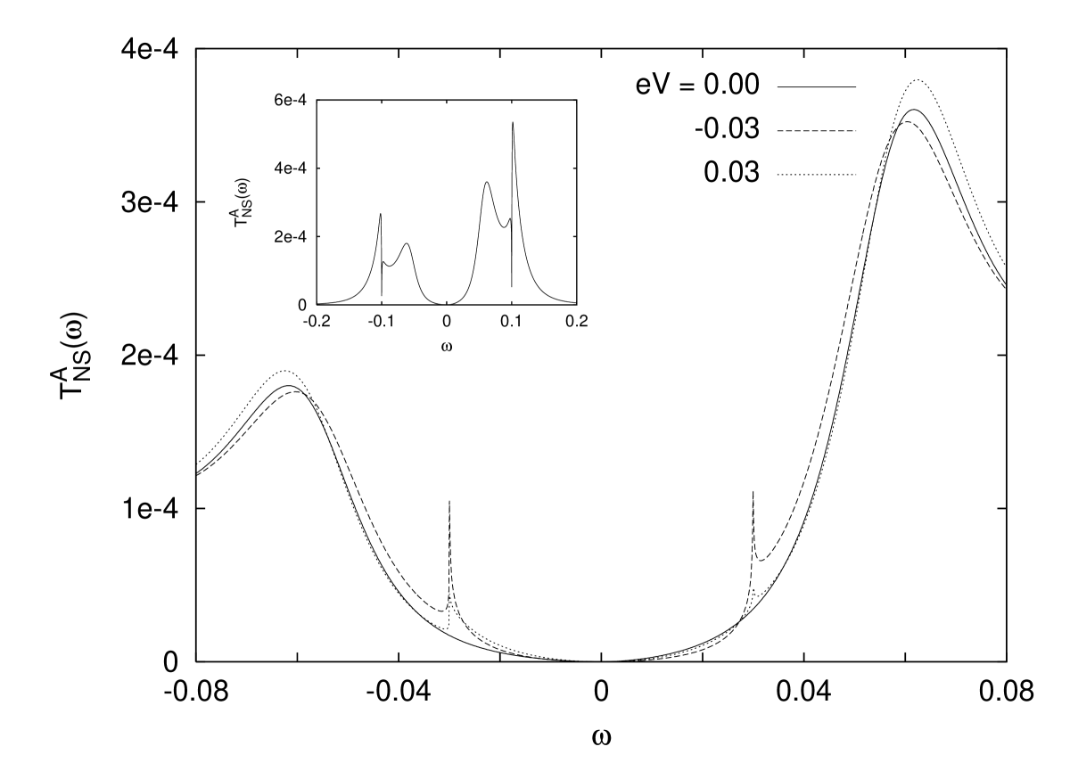
Figure 6: $T^{A}_{NS}(\omega)$ for different values of the bias voltage $eV=0$ (solid line), $-0.03$ (dashed) and $0.03$ (dotted line). $E_{d}=-0.08$, $\Gamma_{N}=\Gamma_{S}=0.01$ and $\Delta=0.1$. Inset: large scale view of the equilibrium $T^{A}_{NS}(\omega)$.

The broad resonances at $\omega\approx\pm 0.06$ are reflections of the dot energy level $E_{d}=0.08$ for electrons and holes [26], shifted from its original position due to renormalization caused by the strong Coulomb interaction. But more important point is that there is no Kondo peak in equilibrium ($eV=0$) transmittance. This is in agreement with Refs. [26, 30]. This is because the imaginary part of the anomalous Green’s function $G_{12}(\omega)$ behaves like $|\omega|$ for $\omega\ll\Delta$ while its real part is proportional to $\omega ln{(\omega)}$ and both vanish for $\omega=0$. And this is sufficient to suppress the Kondo effect. However as soon as we go away from the $eV=0$, we can observe the Kondo peaks at energies $\omega=\pm eV$ with approximately equal spectral weight. However there is strong asymmetry between negative (dashed line) and positive (dotted line) voltages. While in former case we have very well resolved resonances, in the later these resonances are strongly suppressed. This asymmetry is strictly related to the density of states (see Fig. (2)), where we also observe such asymmetry, which is associated with different conditions for the Kondo effect in both cases (note quantity $E_{d}-eV$). The fact, that we observe the Kondo peak for both electrons ($eV$) and for holes ($-eV$) is in contradiction to what has been observed in Ref. [26], where only small kink has emerged for $\omega=-eV$. This is certainly due to different approximation scheme used in calculations.

Since equilibrium transmittance $T^{A}_{NS}(\omega)$ doesn’t show the Kondo peak, we cannot expect it in the differential conductance $G_{A}(eV_{SD})=dJ_{A}/d(eV_{SD})$ with $J_{A}$ defined by (67), since $G_{A}$ is proportional to the equilibrium $T^{A}_{NS}$. Indeed this is what we observe in the (Fig. 7).

Figure 7: The Andreev differential conductance $G_{A}(eV_{SD})=dJ_{A}/d(eV_{SD})$ for different values of the dot energy level $E_{d}=-0.08$ (solid line), $-0.14$ (dashed) and $0.2$ (dotted line). $\Gamma_{N}=\Gamma_{S}=0.01$ and $\Delta=0.1$.

We see, that $G_{A}(eV_{SD})$ is very sensitive to the position of the dot energy level. The larger (negative) $E_{d}$ the smaller conductance. It can be understood as follows. The probability of the Andreev reflections depends on the density of states (for $\omega<\Delta$) of the normal electrode as well as dot itself. The later one is strongly $E_{d}$-dependent (see Fig. 1). For $E_{d}\ll 0$ there are no states on the dot participated in tunneling between normal electrode and the superconductor. Note that in fact Andreev reflections take place between $SC$ electrode and the dot.

The lack of the peak in the differential conductance confirms that the Kondo effect is suppressed in the $N-QD-S$ system with strong on-dot Coulomb repulsion. This result is in full agreement with those of Refs. [26, 30, 32].

5 Asymmetric coupling

The quantum dot asymmetrically coupled to the normal state electrodes shows anomalous Kondo effect [45], which has also been observed experimentally [12, 13]. This anomaly features in the non-zero position of the Kondo resonance in the differential conductance. In other words, if we increase one of the couplings to the leads ($\Gamma_{L}(R)$), the zero-bias anomaly moves to non-zero voltages [45]. In the $N-QD-S$ system, there is no Kondo resonance in the differential conductance. Similarly there is no it in the equilibrium transmittance. On the other hand the Kondo peak emerges when system is in nonequilibrium. So in fact we could expect the non-zero bias Kondo peak in the differential conductance of the dot asymmetrically coupled to the leads.

We have calculated Andreev transmittance and differential conductance for a number of couplings to the leads. The example is shown in the Fig. 8.

Figure 8: The Andreev transmittance $T^{A}_{NS}$ for different values of the couplings to the leads $\Gamma_{N}=\Gamma_{S}=0.01$ (solid line), $\Gamma_{N}=0.015$, $\Gamma_{S}=0.01$ (dashed) and $\Gamma_{N}=0.01$, $\Gamma_{S}=0.015$ (dotted line). $E_{d}=-0.08$ and $\Delta=0.1$.

Unfortunately we haven’t observed the Kondo peak at non-zero voltages regardless how big the asymmetry ($\Gamma_{N}/\Gamma_{S}$) was. The reason for this might be that for $N-QD-N$ system the shift of the Kondo peak to non-zero values is very small [45], and in the present case the Kondo resonance cannot develop because there are too few states in the transmittance spectra around the Fermi energy.

However the asymmetry in the couplings lead to another interesting behavior of the Andreev transmittance as well as differential conductance. Namely it turns out that $\Gamma_{N}$ more influences the $T^{A}_{NS}$ ($G_{A}$) around energies close to value of $SC$ gap than $\Gamma_{S}$ does (see dashed line in the Fig. 8). On the other hand the transmittance (conductance) around $|E_{d}|<\Delta$ is more affected by $\Gamma_{S}$ (compare dotted line in the Fig. 8). We can also note that the positions of the broad resonances, corresponding to the dot energy level $E_{d}$, depend on asymmetry. This is due to the real part of self-energy. More important is that $\Gamma_{N}$ and $\Gamma_{S}$ shift the positions of the resonances in opposite directions: $\Gamma_{N}$ towards Fermi energy $\mu_{N}=\mu_{S}=0$ while $\Gamma_{S}$ to higher energies.

In the present approach the Andreev transmittance (and differential conductance) vanishes at zero energy. However it shows interesting properties at the other characteristic energies of the system, like $E_{d}$ or $\Delta$. The Andreev transmittance $T^{A}_{NS}$ at these energies is shown in the Fig. 9 as a function of the asymmetry in the coupling $\Gamma_{N}/\Gamma_{S}$.

Figure 9: $T^{A}_{NS}$ at energies: $-E_{d}$ (solid line), $E_{d}$ (dashed), $-\Delta$ (dotted) and $\Delta$ (dot-dashed line) as function of the $\Gamma_{N}/\Gamma_{S}$ for $E_{d}=-0.08$, $\Delta=0.1$ and fixed $\Gamma_{N}+\Gamma_{S}=0.02$.

We see that the tunneling due to the Andreev processes at energies $\pm E_{d}$ is likely to take a place when the couplings are more or less symmetric, i. e. $\Gamma_{N}=\Gamma_{S}$. More surprising result is that the largest probability of these processes at energies $\pm\Delta$ is for large asymmetry $\Gamma_{N}/\Gamma_{S}\approx 10$. As we already mentioned such behavior can be explained by renormalization of the dot energy level due to the real part of self-energy, which depends on $\Gamma_{N}$ and $\Gamma_{S}$ in rather a complicated way .

6 Particle-hole asymmetry

Until now we have presented results for the special case, namely the electron-hole ($e-h$) symmetry in the leads. It is well known [46] that the particle-hole asymmetry in the normal metal/superconductor tunnel junctions and metallic contacts suppresses the Andreev reflections due to the fact that the reflection and transmission probabilities are different for incident electrons and holes. In the quantum dot coupled to the normal and superconducting electrode we could also expect that this asymmetry will play a role. On the other hand, this asymmetry is already present in the strongly interacting quantum dot ($U=\infty$) in the Kondo regime ($E_{d}<0$), as one studied here. However this asymmetry in the leads can further modify the Andreev tunneling.

Let’s start from the effect of the $e-h$ asymmetry on the density of states. As we can read from the Fig. 10, the asymmetry plays rather a minor role.

Figure 10: Density of states in various realizations of the electron-hole asymmetry indicated in the figure. Parameters have following values: $E_{d}=-0.08$, $\Delta=0.01$, $\Gamma_{N}=\Gamma_{S}=0.01$.

The most pronounced difference is when the concentration in both $N$ and $S$ electrodes are changed. If change the concentration in one of the electrode, the effect is smaller. Moreover, the density of states almost does not depend on in which electrode concentration is changed. In other words, it seems to be sensitive to average concentration in both electrodes.

In the Fig. 11 we have shown the height of the Kondo resonance when electron concentration is varied.

Figure 11: The height of the Kondo peak as a function of the concentrations of the electrons $n_{N}$ ($n_{S}$) in the normal (superconducting) lead. Curve $N,S$ - electron concentration in both electrodes is changed, $N$ - in the normal electrode only and $S$ - in superconducting. The parameters are the same as in Fig. 10.

As one can read from the Fig. 11, the spectral weight of the Kondo peak strongly depends on the electron concentration in both electrodes. Moreover there is a strong asymmetry with respect to the $n=1$ point, i. e. the peak is higher when the concentration of electrons is higher. It is rather expected result, as in the original Kondo effect the resonance at zero energy emerges due to the screening of the conduction electrons. So one could expect that it should depend on their concentration, as it does. Similar effect we observe when the electron concentration is changed in one lead only. It almost does not depend on in which lead $n$ is changed. However for large $e-h$ asymmetry, concentration of electrons in the normal lead seems to play a more important role.

Now let’s turn to the Andreev reflections and their modifications due to the $e-h$ asymmetry. The Andreev transmittance $T^{A}_{NS}(\omega)$ (Eq. (69)), shown in the Fig. 12 is also affected by the concentration of the electrons in the leads.

Figure 12: Andreev transmittance for various electron concentrations in the leads. Model parameters are the same as in Fig. 10.

However quantitative behavior of $T^{A}_{NS}(\omega)$ seems to not depend on the $e-h$ asymmetry. The most pronounced qualitative differences occur for the energies $\omega=|E_{d}|$. Decreasing the number of electrons in the normal lead, $T^{A}_{NS}(\omega)$ also decreases around these energies. On the other hand, the effect is just opposite if we decrease the electron concentration in the $SC$ lead. One can rather easily explain the dependence of the $T^{A}_{NS}(\omega)$ on the number of normal electrons, taking note of the fact that probability of Andreev reflections is larger when number of electrons in $N$ lead is large and the number of holes small. However $T^{A}_{NS}(\omega)$ also depends on concentration of electrons and holes in the $SC$ lead. This can be understood as follow: the number of electron-like (hole-like) quasiparticles in $SC$ is proportional to the concentration of the electrons (holes) in this lead in the normal state. In the Andreev process, if two electrons enter the $SC$, the electron-like quasiparticle is created. This means that probability of Andreev reflections depends on the number of electron-like and hole-like quasiparticles in $SC$ lead. So increasing the number of holes in $SC$, the probability of Andreev reflections of the impinging electrons is larger. This is exactly what we can read from the Fig. 12.

The modifications of the $T^{A}_{NS}(\omega)$ due to $e-h$ asymmetry are not so large as the modifications due to the asymmetry in the couplings (see Fig. 8), nevertheless $e-h$ asymmetry influences the Andreev tunneling.

7 Conclusions

In conclusion we have studied a strongly interacting quantum dot connected to the normal and superconducting leads. Using the equation of motion technique for the nonequilibrium Green’s functions, we derived the formula for the current in terms of various tunneling processes. This technique allowed us to calculate at once all the Green’s functions emerging in the problem and perform consistent decoupling procedure for the higher order Green’s functions.

We discussed the problem of the interplay between Kondo effect and Andreev reflections. While the Kondo resonance is present in density of states, there is no zero bias anomaly in the differential conductance. As a matter of fact, the Andreev conductance is strongly suppressed for zero-bias voltages. We also further raised a question regarding the participation of the superconducting electrons in the Kondo effect. The obtained results seem to support the scenario in which they do not participate in the Kondo effect.

Finally, we discussed the problem of asymmetry in the couplings to the leads and found the large modifications of the Andreev conductance due to this effect, mainly for energies around dot level and superconducting gap. We also studied the properties of the system when the concentration of electrons in the leads can be changed. However, the modifications of the Andreev tunneling due to this effect are much smaller and quantitative only.

References

References

- [1] D. K. Ferry, S. M. Goodnick, Transport in Nanostructures, Cambridge University Press, Cambridge (1997).
- [2] L. I. Glazman, M. E. Raikh, JETP Lett. 47, 452 (1988).
- [3] T. K. Ng, P. A. Lee, Phys. Rev. Lett. 61, 1768 (1988).
- [4] A. Kawabata, J. Phys. Soc. Jpn. 60, 3222 (1991).
- [5] S. Herschfield, J. H. Davies, J. W. Wilkins, Phys. Rev. Lett. 67, 3720 (1991); S. Herschfield, J. H. Davies, J. W. Wilkins, Phys. Rev. B46, 7046 (1992).
- [6] Y. Meir, N. S. Wingreen, P. A. Lee, Phys. Rev. Lett. 66, 3048 (1991); ibid. 70, 2601 (1993).
- [7] A. Levy Yeyati, A. Martín-Rodero, F. Flores, Phys. Rev. Lett. 71, 2991 (1993).
- [8] N. S. Wingreen, Y. Meir, Phys. Rev. B49, 11 040 (1994).
- [9] M. H. Hetller, H. Schoeller, Phys. Rev. Lett. 74, 4907 (1995).
- [10] D. Goldhaber-Gordon, H. Shtrikman, D. Mahalu, D. Abush-Maggder, U. Meirav, M. A. Kastner, Nature 391, 156 (1998).
- [11] S. M. Cronenwett, T. H. Oosterkamp, L. P. Kouwenhoven, Science 281, 540 (1998).
- [12] J. Schmid, J. Weis, K. Eberl, K. von Klitzing, Physica B256-258, 182 (1998); J. Schmid, J. Weis, K. Eberl, K. von Klitzing, Phys. Rev. Lett. 84, 5824 (2000).
- [13] F. Simmel, R. H. Blick, J. P. Kotthaus, W. Wegsheider, M. Bichler, Phys. Rev. Lett. 83, 804, (1999).
- [14] S. Sasaki, S. De Franceschi, J. M. Elzerman, W. G. van der Wiel, M. Eto, S. Tarucha, L. P. Kouwenhoven, Nature 405, 764 (2000).
- [15] A. F. Andreev, Sov. Phys. JETP 19, 1228 (1964).
- [16] C. J. Lambert, R. Raimondi, J. Phys. Condens. Matter 10, 901 (1998); T. Löfwander, V. S. Shumeiko, G. Wendin, Supercond. Sci. Technol. 14, R53 (2001).
- [17] C. W. J. Beenakker, Phys. Rev. B46, 12 841 (1992).
- [18] N. R. Claughton, M. Leadbeater, C. J. Lambert, J. Phys. Condens. Matter 7, 8757 (1995); M. Leadbeater, N. R. Claughton, C. J. Lambert, V. N. Prigodin, Surf. Science 361-362, 302 (1996).
- [19] L. P. Kouwenhoven, P. L. McEuen, in: G. Timp(Ed.), Nanotechnology, Springer, New York, 1999.
- [20] Q. Sun, J. Wang, T. Lin, Phys. Rev. B59, 3831 (1999).
- [21] J. -F. Feng, S. -J. Xiong, J. Phys. Condens. Matter 14, 3641 (2002).
- [22] H. Zhao, G. v. Gehlen, Phys. Rev. B58, 13 660 (1998).
- [23] H. Zhao, Phys. Lett. A264, 218 (1999).
- [24] Y. Zhu, Q. Sun, T. Lin, Phys. Rev. B64, 134521 (2001).
- [25] Y. Zhu, Q. Sun, T. Lin, Phys. Rev. B65, 024516 (2002).
- [26] R. Fazio, R. Raimondi, Phys. Rev. Lett. 80, 2913 (1998); ibid. 82, 4950 (1999).
- [27] P. Schwab, R. Raimondi, Phys. Rev. B59, 1637 (1999).
- [28] R. Raimondi, P. Schwab, Superlatt. Mictrostruct. 25, 1141 (1999).
- [29] K. Kang, Phys. Rev. B58, 9641 (1998).
- [30] A. A. Clerk, V. Ambegaokar, S. Hershfield, Phys. Rev. B61, 3555 (2000).
- [31] Y. Avishai, A. Golub, A. D. Zaikin, Phys. Rev. B63, 134515 (2001).
- [32] J. C. Cuevas, A. Levy Yeyati, Martín-Rodero, Phys. Rev. B63, 094515 (2001).
- [33] Q. Sun, H. Guo, T. Lin, Phys. Rev. Lett. 87, 176601 (2001).
- [34] P. W. Anderson, Phys. Rev. 124, 41 (1961).
- [35] L. V. Keldysh, Zh. Eksp. Teor. Fiz. 47, 1515 (1965) [Sov. Phys. JETP 20, 10 108 (1965)].
- [36] H. Haug, A. P. Yauho, Quantum Kinetics in Transport and Optics of Semiconductors, Springer, Berlin, 1996.
- [37] T. K. Ng, Phys. Rev. Lett. 76, 487 (1996).
- [38] C. Niu, D. L. Lin, T. -H. Lin, J. Phys. Condens. Matter 11, 1511 (1999).
- [39] M. Krawiec, K. I. Wysokiński, Solid State Commun. 115, 141 (2000).
- [40] S. E. Barnes, J. Phys. F6, 1375 (1976); J. Phys. F7, 2631 (1977).
- [41] P. Coleman, Phys. Rev. B29, 3035 (1984).
- [42] J. C. Le Guillou, E. Ragoucy, Phys. Rev B52, 2403 (1995).
- [43] M. Krawiec, K. I. Wysokiński, Phys. Rev. B60, 9500 (1999).
- [44] G. E. Blonder, M. Tinkham, T. M. Klapwijk, Phys. Rev. B25, 4515 (1982).
- [45] M. Krawiec, K. I. Wysokiński, Phys. Rev. B66, 165408 (2002).
- [46] J. E. Hirsch, Phys. Rev. B50, 3165 (1994).