Confinement control by optical lattices

Abstract

It is shown that the interplay of a confining potential with a periodic potential leads for free particles to states spatially confined on a fraction of the total extension of the system. A more complex “slicing” of the system can be achieved by increasing the period of the lattice potential. These results are especially relevant for fermionic systems, where interaction effects are in general strongly reduced for a single species at low temperatures.

I Introduction

The study of trapped atomic gases has become a field of intense research in the past years. The realization of Bose-Einstein condensation (BEC) in trapped dilute atomic vapors anderson ; bradley ; davis was the main motivation starting all the experimental and theoretical research in this area. BEC was obtained trapping and evaporatively cooling bosonic alkali metals. Recently, the possibility of trapping and cooling Fermi gases has attracted a lot of attention, due to the fact that in the quantum degeneracy regime, superfluidity appears within reach ohara . However, cooling single component Fermi gases up to very low temperatures is more difficult than cooling bosonic gases since the $s$-wave collisions are forbidden for identical fermions. On the other hand, single species Fermi gases make in this way possible to access experimentally an ideal Fermi gas. As shown below, such a simple system can develop a rich behavior by the combination of a confining and a lattice potential.

For atoms confined in a harmonic trap, a case that adequately describes most of the experiments realized so far dalfovo , a fairly complete theoretical understanding was achieved for the one-dimensional (1D) gleisberg ; vignolo1 ; minguzzi ; vignolo2 and two- or three-dimensional schneider ; brack ; vignolo3 single component spin polarized trapped Fermi gas, which at very low temperatures can be considered as a noninteracting gas. The harmonic form of the potential allows obtaining a number of exact analytical results for these systems. However, these results cannot be extended to incorporate an additional lattice potential, a case of increasing interest after the experimental realization of a Mott insulator in the presence of an optical lattice greiner . A further interest on the introduction of an optical lattice in fermionic systems arises from the possible connections with central problems in condensed matter physics zoller .

We analyze here ground state properties of single species noninteracting fermions confined on 1D optical lattices. These systems are relevant for the understanding of recent experimental results modugno03 ; ott04 ; pezze04 , where due to the very low temperatures achieved, fermions can be considered as noninteracting particles. On the theoretical side, the Hamiltonian can be diagonalized numerically, which allows to consider any kind of trapping potential and any number of dimensions for the system. We show that the interplay between the lattice and the confining potential leads in a region of the spectrum to a splitting of the system with eigenstates that have a nonvanishing weight only in a fraction of the trap. Hence, such systems are qualitatively different from the cases without the lattice, which have been studied recently gleisberg ; vignolo1 ; minguzzi ; vignolo2 ; schneider ; brack ; vignolo3 .

We also study the nonequilibrium dynamics of the fermionic cloud on a lattice. In particular, we study the case in which the center of the trap is initially displaced a small distance. It allows to realize the existence of the single particle states confined in a part of the trap obtained in the equilibrium case, since for some values of the parameters the center-of-mass (c.m.) of the system oscillates in one side of the trap. With these results, we reproduce the experimental observations in Refs. modugno03 ; ott04 ; pezze04 , and complement other theoretical approaches to this problem pezze04 ; kennedy04 ; ruuska04 .

We show that if in addition to the lattice an alternating potential is introduced, doubling the original periodicity, an additional “slicing” of the system can be achieved. The width and number of such regions can be controlled in a given energy range by the amplitude of the new modulation. By filling these systems with fermions, insulating regions may appear, that in the case of an alternating potential, are similar to the Mott insulating plateaus of the trapped fermionic Hubbard model rigol03_1 ; rigol03_2 . In the noninteracting case it is possible to calculate the local density of states, which exhibits the presence of a local gaps in the system. In addition, a local compressibility rigol03_1 ; rigol03_2 also serves as a local order parameter to characterize the insulating regions. This extends the results initially obtained for the bosonic case batrouni , showing that in general, the distinction between commensurate and incommensurate fillings typical in extended solid-state systems is lost in the trapped system.

The presentation is organized as follows: In Sec. II we study 1D lattices superposed to a confining potential. We analyze the generic features valid for any kind of trapping potential, and focus on fermionic systems. In Sec. III, an analysis of the nonequilibrium dynamics of the 1D trapped fermions is presented, and recent experimental results reproduced. In Sec. IV we study the case in which an additional alternating potential in introduced, and dicuss analogies and differences with the results obtained for the fermionic Hubbard model. In Sec. IV, we extend the analysis of Sec. II and IV to two dimensions (2D). Finally the conclusions are given in Sec. V.

II Noninteracting particles confined in 1D optical lattices

We analyze in this section 1D noninteracting systems confined by arbitrary potentials when an underlying optical lattice is present. We first show results for a harmonic confining potential and then discuss the features that are generally valid for any other kind of confining potential. For definiteness we concentrate on the fermionic case, although the spectral features are equally valid for bosons, since we deal with the noninteracting case.

In the second quantization language, the Hamiltonian describing a confined dilute and ultracold (noninteracting) gas of single-species fermions, under the influence of a 1D optical lattice, can be written as

$$H=\int d{\bf r}\ \hat{\Psi}^{\dagger}({\bf r})\left[-\dfrac{\hbar^{2}}{2m}\nabla^{2}+V({\bf r})+V_{0}(x)\right]\hat{\Psi}({\bf r}),$$ (1)

where $\hat{\Psi}^{\dagger}({\bf r})$ and $\hat{\Psi}({\bf r})$ are the creation and annihilation fermionic field operators, respectively. The confining potential is denoted as $V({\bf r})=V(x)+V(y)+V(z)$. We analyze in this section the case in which the transversal component of the confining potential $V(y)+V(z)$ is very strong so that only its lowest energy state is populated, and the exited states are not accessible for the given experimental setup. Hence, the relevant dynamics of the system is restricted to occur in the longitudinal direction where the trap is considered to have an arbitrary power $\alpha$, $V(x)=V_{\alpha}x^{\alpha}$. In Eq. (1), $V_{0}(x)=V_{0}\cos^{2}(kx)$ describes the potential generated by a 1D optical lattice. The wave vector $k=2\pi/\lambda$ is determined by the wavelength $\lambda$ of the laser beam. (The lattice spacing is then $a=\lambda/2$.) Assuming the atoms to be at the lowest vibrational level in each site, the fermionic field operators can be expanded in single band Wannier functions $\phi_{i}(x)$, $\hat{\Psi}(x)=\sum_{i}c_{i}\phi_{i}(x)$, and from Eq. (1) one obtains the single band Hamiltonian

$$H=-t\sum_{i}\left(c^{\dagger}_{i}c_{i+1}+\text{H.c.}\right)+V_{\alpha}\sum_{i}x_{i}^{\alpha}\ n_{i},$$ (2)

where $c^{\dagger}_{i}$ and $c_{i}$ are creation and annihilation operators, respectively, for a spin polarized fermion on site $i$, the local density is $n_{i}=c^{\dagger}_{i}c_{i}$, and $x_{i}$ measures the positions of the sites in the trap ($x_{i}=ia$ with $-N/2+1\leq i\leq N/2$, $N$ being the number of lattice sites). The hopping parameter is denoted by $t$, which for $V_{0}\gg E_{r}$ can be written in terms of the experimental parameters as $t=4/\sqrt{\pi}(V_{0}/E_{r})^{3/4}E_{r}e^{-2\sqrt{V_{0}/E_{r}}}$ zwerger , where the recoil energy of the atoms (with mass $m$) is $E_{r}=\hbar^{2}k^{2}/2m$. The total number of spin polarized fermions in the system is denoted by $N_{f}$. We diagonalize the Hamiltonian numerically, and consider the cases in which all particles are confined.

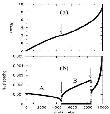
Figure 1: Single particle spectrum (a) and level spacing (b) for a system with $N=10000$ and $V_{2}a^{2}=3\times 10^{-7}t$. Energies are measured in units of $t$. For the explanation of the arrows see text.

Results obtained for the single particle spectrum of a system confined by a harmonic potential are presented in Fig. 1(a). The spectrum is clearly different from the usual straight line in the absence of a lattice. It is possible to see that in Fig. 1(a) the spectrum can be divided in two regions according to the behavior of the energy as a function of the level number. An arrow is introduced where a change in the curvature is observed. More detailed information can be obtained by considering the level spacing as a function of the level number [Fig. 1(b)]. There it can be seen that in the low energy part of the spectrum (region A), the level spacing decreases slowly with increasing level number, in contrast to the case without the lattice in which the level spacing is constant. However, at the point signaled with the first arrow, a qualitative change in the single particle spectrum occurs, characterized by an oscillating behavior of the level spacing. The part with values of the level spacing increasing with the level number corresponds to odd level numbers and the one with a level spacing that decreases up to zero corresponds to even level numbers. That is, a degeneracy sets in that continues up to the point signaled with the second arrow, where a new change in the behavior of the level spacing shows up. The region beyond the second arrow corresponds to deconfined states, which are of no interest since experimentally they are associated to particles that scape from the trap (which in the system of Fig. 1 has 10000 lattice sites).

In the lowest part of the spectrum of Hamiltonian (2), the eigenfunctions are essentially the harmonic oscillator (HO) orbitals in the absence of a lattice. This is shown in Fig. 2(a) for the first and the second eigenfunctions of Eq. (2), and the same parameters of Fig. 1. These orbitals are perfectly scalable independently of the size of the system and of the ratio between $V_{2}$ and $t$. It is only needed to consider that the usual HO characteristic length $R\sim\left(m\omega\right)^{-1/2}$ (without the lattice) is given in terms of the lattice parameters through $R\sim\left(V_{2}/ta^{2}\right)^{-1/4}$, with the effective mass $m\sim\left(ta^{2}\right)^{-1}$ for very low energies, so that the scaled orbitals are given by $\varphi=\left(R/a\right)^{1/2}\phi$ where $\phi$ are the HO orbitals with the lattice, i.e., the same relation as for the HO without the lattice holds for the lowest energy orbitals with the periodic potential. This implies that very dilute systems behave similarly to continuous systems, which have been already discussed in the literature so that we do not present any further analysis on them. The $N_{f}$ oscillations in density profiles and momentum distribution function (MDF), and other mentioned characteristics of the 1D trapped system without the lattice vignolo1 ; minguzzi are easily obtained in this case.

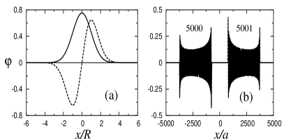
Figure 2: Scaled HO orbitals in the presence of a lattice for $N=10000$ and $V_{2}a^{2}=3\times 10^{-7}t$. (a) First (continuous line) and second (dashed line) HO orbitals, (b) HO orbitals 5000 (only different from zero for negative $x$) and 5001 (only different from zero for positive $x$). In (a) the positions are given in units of the HO length $R=\left(V_{2}/ta^{2}\right)^{-1/4}$ (for an explanation, see text), and in (b) in units of the lattice constant $a$.

A qualitative difference between the cases of the trap with and without a lattice starts for levels in region B. Once the degeneracy appears in the spectrum, the corresponding eigenfunctions of the degenerate levels start having zero weight in the middle of the trap, and for higher levels the regions over which the weight is zero increases. As an example, we show in Fig. 2(b) two normalized eigenfunctions belonging to region B in Fig. 1. The cases depicted correspond to the normalized eigenfunctions 5000 (that is only different from zero for negative values of $x$) and 5001 (only different from zero for positive $x$), for the same parameters of Fig. 1 (in principle a lineal combination of these two eigenfunctions could have been the solution since the level is degenerated). Hence, particles in these states are confined to a fraction of the trap, showing that the combination of both a confining and a periodic potential lead to features not present either in the purely confined case without a lattice or in the case of a purely periodic potential. Furthermore, since we are dealing with a noninteracting case, such features are common to both fermions and bosons. However, in the case of fermions, it is easy to understand the reason for such effects, as discussed next.

Figure 3(a) shows density profiles of fermions when the number of particles in the trap is increased. In one case ($N_{f}=4500$) the Fermi energy lies just below the level marked with an arrow in Fig. 1. A second curve ($N_{f}=4651$) corresponds to the case where the central site reaches a density $n=1$, and in the other case ($N_{f}=5001$), the Fermi energy lies at the value corresponding to the levels depicted in Fig. 2(b). The positions in the trap are normalized in terms of the characteristic length for a trapped system when a lattice is present, which is given by rigol03_1 ; rigol03_2

$$\zeta=\left(V_{2}/t\right)^{-1/2}.$$ (3)

When the Fermi energy approaches the level where degeneracy sets in, the density of the system approaches $n=1$ in the middle of the trap, and at the filling point where the degeneracy appears in the spectrum, the density in the middle of the trap is equal to one, so that an insulating region appears in the middle of the system. Increasing the filling of the system increases the region over which this insulator extends. Hence, due to Pauli principle, the eigenfunctions of such levels cannot extend over the insulating region, and for the same reason, the region over which the weight is zero increases for higher levels. The local insulator with $n=1$ has zero variance of the density and, it is incompressible, a property that could be tested experimentally by using a local probe.

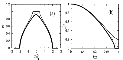
Figure 3: Density profiles (a) and normalized MDF (b) for $N_{f}=4500$ (thick continuous line), $N_{f}=4651$ (dashed line), and $N_{f}=5001$ (think continuous line) for a system with $N=10000$ and $V_{2}a^{2}=3\times 10^{-7}t$. In (a) the positions are given in units of the characteristic length $\zeta$, and in (b) the momentum is normalized by the lattice constant $a$.

However, since the system we are considering is a noninteracting one, the confined states discussed above should be also present in the case of bosons, where the argument about the filling would not be valid anymore. It is therefore desirable to also understand such features from a single particle perspective pfau . We first notice that the point at which degeneracy appears is at an energy $4t$ above the lowest level ($E_{0}$) [see Fig. 1(a)], corresponding to the bandwidth for the periodic potential. Such an energy is reached when the Bragg condition is fulfilled and in the case of the tight-binding system we are considering, when all the available states are exhausted. Let us next consider the case depicted in Fig. 2(b). There, the energy level corresponding to the wave functions is $E_{5001}-E_{0}=4.2176t$, that is to a good approximation $4t+V_{2}x_{1}^{2}$ for $V_{2}a^{2}=3\times 10^{-7}t$ and $x_{1}=697a$ the inner point where the wave functions drop to a value $\sim 10^{-5}$. Therefore, the inner turning point corresponds to the Bragg condition, whereas for the outer turning point ($x_{2}=3770a$, again for the same drop of the wave function), we have that $E_{5001}-E_{0}\simeq V_{2}x_{2}^{2}$, i.e., the classical turning point corresponding to the harmonic potential, as expected for such a high level. Hence, Bragg scattering as in the well known Bloch oscillations zener34 , and the trapping potential combine to produce the confinement discussed here.

Further confirmation of the argument above can be obtained by considering the MDF, a quantity also accessible in time of flight experiments greiner . Due to the presence of a lattice, it is a periodic function in the reciprocal lattice kaskurnikov and it is symmetric with respect to $k=0$, so that we study it in the first Brillouin zone in the region [$0,\ \pi/a$]. In addition we normalize the MDF to unity at $k=0$ ($n_{k=0}=1$). For the fermionic case, it can be seen that it always has a region with $n_{k}=0$ if the insulating phase is not present in the trap, and this region disappears as soon as the insulator appears in the middle of the system. More precisely, Fig. 3(b) shows that at the filling when the site in the middle reaches $n=1$, also the momentum $k=\pi/a$ is reached, such that the Bragg condition is fulfilled for the first time, confirming the discussion above. When further sites reach a density $n=1$, $n_{k=\pi/a}$ increases accordingly. Then the formation of the local insulator in the system can be tested experimentally observing the occupation of the states with momenta $k=\pm\pi/a$.

Since for different systems sizes and number of particles, potentials with different curvatures have to be considered, it is important to determine the filling $N_{f}^{C}$ at which the insulator appears in the middle of the trap as a function of the curvature of the harmonic confining potential. This question was already answered for the interacting case (Hubbard model) in Refs. rigol03_1 ; rigol03_2 where we determined the phase diagram. There we showed that if a dimensionless characteristic density $\tilde{\rho}$ is defined as $\tilde{\rho}=N_{f}a/\zeta$, then its value when the insulating regions (Mott insulating and band insulating in the interacting case) appear in the system is always constant for any value of $V_{2}/t$ at a given value of $U/t$ (within error bars there), so that $N^{C}_{f}\sim\zeta/a$. However, in Refs. rigol03_1 ; rigol03_2 we were able to check this only up to 150 lattice sites and fillings up to the same order, whereas here we extend those results to much larger systems. In Fig. 4(a) we show in a log-log scale how $N^{C}_{f}$ depends on $V_{2}/t$ over three decades on the total filling. In our fit the slope of the curve is $-0.500$ (with 0.04 percent of error), as expected on the basis of Eq. (3). The critical characteristic density ${\tilde{\rho}}_{C}=N_{f}^{C}a\left(V_{2}/t\right)^{1/2}$ at which the insulating region appears is ${\tilde{\rho}}_{C}={\rm e}^{\beta}$, with $\beta=0.986$ (with 0.3 percent of error), which is curiously rather close to the basis of the natural logarithms.

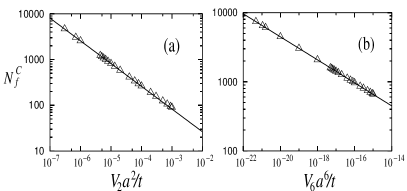
Figure 4: Total filling in the trap needed for the formation of the insulator as a function of the curvature of the confining potential. (a) Harmonic potential. (b) Potential with a power $\alpha=6$.

For systems with other powers for the confining potential it is only needed to define the appropriate dimensionless characteristic density $\tilde{\rho}=N_{f}a\left(V_{\alpha}/t\right)^{1/\alpha}$, and determine its value at the point where the insulator appears. In Fig. 4(b) we show in another log-log plot how $N_{f}^{C}$ depends on the curvature of a confining potential with power six ($V_{6}/t$). As anticipated, we obtain that the slope of the curve is $1/6$ (with 0.01 percent of error) in this case and the characteristic density for the formation of the insulator is ${\tilde{\rho}}_{C}=2.09$. Finally, we should mention that it was already shown in Ref. rigol03_2 that keeping constant the characteristic density but changing the curvature of the confining potential and the total filling in the trap, the density profiles as a function of the normalized coordinate and the normalized MDF remain unchanged.

In general, for arbitrary confining potentials the same features discussed previously for the harmonic case are valid. The spectrum and level spacing behave in a different way depending on the power of the confining potential, but always at a certain level number degeneracy appears in the single particle spectrum and it corresponds to the formation of an insulator in the middle of the system for the corresponding filling. In Fig. 5 we show the single particle spectrum [Fig. 5(a)] and the corresponding level spacing [Fig. 5(b)] for a confining potential with power $\alpha=6$, where the features mentioned previously are evident. The arrow in the inset of Fig. 5 shows the level at which degeneracy sets in, very much in the same way as in the harmonic case.

Figure 5: Single particle spectrum (a) and level spacing (b) for a system with a confining potential with power $\alpha=6$, $N=28000$, and $V_{6}a^{6}=3\times 10^{-7}t$. Energies are measured in units of $t$. Expanded view in (b) shows the first part of the level spacing. An arrow was introduced in the inset for signaling the level at which the degeneracy appears in the spectrum.

We close this section by considering the pair distribution function. This quantity not only reflects the consequences of Pauli’s exclusion principle but clearly characterizes the insulating region. In the presence of a lattice the pair distribution function can be written as

$$P_{ij}=\langle n_{i}\rangle\langle n_{j}\rangle-\rho_{ij}^{2},$$ (4)

where $\rho_{ij}=\langle c_{i}^{\dagger}c_{j}\rangle$ is the fermionic one-particle density matrix.

In Fig. 6 we show as intensity plots the pair distribution function for systems with $N=1000$ lattice sites and $V_{2}a^{2}=3\times 10^{-5}t$. Figure 6(a) corresponds to the case with $N_{f}=300$ fermions, where the systems is completely metallic, whereas Fig. 6(b) corresponds to $N_{f}=600$ fermions, an insulating region appears in the middle of the trap. Apart from the depression along the diagonal that reveals the consequences of Pauli’s exclusion principle, a clear distinction between the purely metallic case and the one with an insulating region can be seen. Inside the insulating region, the density matrix becomes diagonal, such that $P_{ij}=1$ for $i\neq j$ and $P_{ii}=0$.

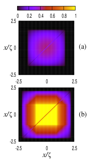
Figure 6: (Color online) Intensity plots of the pair distribution function as a function of the normalized position for (a) $N_{f}=300$ (only a metal is present in the trap) and (b) $N_{f}=600$ (a insulating region is formed in the middle of the trap). The number of lattice sites is $N=1000$ and $V_{2}a^{2}=3\times 10^{-5}t$.

III Oscillations of fermions in a 1D lattice

Recent experiments have realized single species noninteracting fermions in 1D optical lattices modugno03 ; ott04 ; pezze04 . Transport studies in such systems revealed that under certain conditions a sudden displacement of the trap center is followed by oscillations of the c.m. of the fermionic cloud in one side of the trap. This is in contrast to the system without the lattice where the c.m. oscillates, as expected, around the potential minimum modugno03 ; ott04 ; pezze04 . Although the experimental system is not a true 1D system, due to the strong transversal confinement the relevant motion of the particles occurs in the longitudinal direction. Hence, in order to qualitatively understand the observed behavior one can analyze the ideal 1D case. Given the results discussed in the previous section one expects the displaced oscillation of the c.m. to appear when, due to the initial displacement of the trap, particles that where located in region A of the spectrum in Fig. 1(b) are moved into region B so that Bragg conditions are fulfilled. Then the particles get trapped in one side of the system [Fig. 2(b)].

Figure 7 shows exact results obtained for the c.m. dynamics of 1000 fermions in a trap with $N=3000$ when its center is suddenly displaced 200 lattice sites. $\tau$ denotes the real time variable. The relation between the confining potential ($V_{2}$) and the hopping parameter ($t$) is increased in order to fulfill the Bragg conditions. This is equivalent in experiments to increase the curvature of the confining potential keeping constant the depth of the lattice, which leads to an increase of the frequency of the oscillation as shown in Fig. 7. It is also equivalent to increase the depth of the lattice keeping the confining potential constant, but then our plots in Fig. 7 should be interpreted with care since there we normalize the time variable by the hopping parameter, which changes in the latter case.

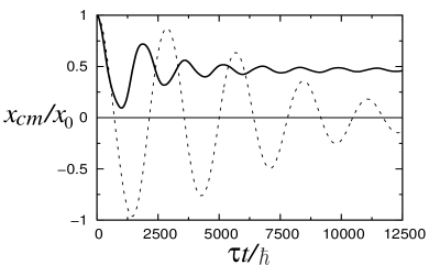
Figure 7: Evolution of the c.m. ($x_{cm}$) of 1000 confined fermions when the center of the trap is suddenly displaced 200 lattice sites ($x_{0}$), for $V_{2}a^{2}=2\times 10^{-06}t$ (dashed line), and $V_{2}a^{2}=6\times 10^{-06}t$ (continuous line).

In Fig. 7 (dashed line) we show results for the case where the c.m. of the cloud oscillates around the minimum of energy of the trap since no Bragg conditions are fulfilled. This can be seen in the MDF [Fig. 8(a)] where at any time no particles have $k=\pm\pi/a$. Figure 7 also shows that a damping of the oscillation of the c.m. occurs. This is due to the nontrivial dispersion relation in a lattice $\epsilon_{k}=-2t\cos ka$, which makes the frequency of oscillation of the particles dependent on their energies, leading to dephasing. In order to reduce the damping, fermions should populate after the initial displacement only levels with energies close to the bottom of the band in a lattice, so that the quadratic approximation is valid for $\epsilon_{k}$. (Notice that this is not generally fullfiled even if the initial displacement is small.)

Figure 8: MDF of 1000 trapped fermions at three different times after displacing the trap 200 lattice sites, for $V_{2}a^{2}=2\times 10^{-06}t$ (a), and $V_{2}a^{2}=6\times 10^{-06}t$ (b). The times are $\tau=0$ (dotted line), $\tau=250\hbar/t$ (dashed line), and $\tau=12500\hbar/t$ (continuous line).

Increasing the relation $V_{2}/t$ makes that some particles start to fulfill the Bragg conditions so that the center of oscillations of the cloud depart from the middle of the trap. In Fig. 7 (continuous line) we show a case where the c.m. never crosses the center of the trap. The MDF corresponding to this case, at three different times, is displayed in Fig. 8(b). There it can be seen that initially ($\tau=0$) no Bragg conditions are satisfied in the system, and that some time after the initial displacement the Bragg conditions are fulfilled ($\tau=250\hbar/t$). Finally, we also show the MDF long time after the initial displacement of the trap ($\tau=12500\hbar/t$), when the oscillations of the c.m. are completely damped and the MDF is approximately symmetric around $k=0$.

IV Doubling the periodicity

In this section we study the consequences of enlarging the periodicity in the lattice. For this purpose we introduce an alternating potential, and the Hamiltonian of the system can be written as

$$H = -t\sum_{i}\left(c^{\dagger}_{i}c_{i+1}+\text{H.c.}\right)+V_{\alpha}\sum_{i}\left(x_{i}\right)^{\alpha}\ n_{i}$$ (5)

$$+V_{a}\sum_{i}\left(-1\right)^{i}\ n_{i},$$

where the last term represents the oscillating potential and $V_{a}$ its strength. The purpose of introducing an alternating potential in the trapped system is twofold. For fermionic systems, the increase of the numbers of sites per unit cell leads to the possibility of creating insulating states (band insulators in the unconfined case) for commensurate fillings. On the other hand, by changing the periodicity, new Bragg conditions are introduced, giving the possibility of further control on the confinement discussed in the previous sections.

Figure 9 shows how the density profiles evolve in a harmonic trap when the total filling is increased. Since the density oscillates due to the alternating potential, we made two different plots for the odd [negative value of the alternating potential, Fig. 9(a)] and even [positive value of the alternating potential, Fig. 9(b)] sites. Each of the plots in Fig. 9 is very similar to the evolution of the density profiles already shown for the trapped Hubbard model rigol03_1 ; rigol03_2 . The only difference is that in Figs. 9(a) and 9(b) the plateaus with $n\neq 1$ have densities different between themselves and different from $n=0.5$, which would be the density of one component of the spin polarized fermions in the Mott insulating phase of the Hubbard model. In the flat regions of Fig. 9, both even and odd sites have the same densities than the corresponding sites in the periodic case at half filling for the same value of the alternating potential, so that it is expected that they correspond to local insulating phases.

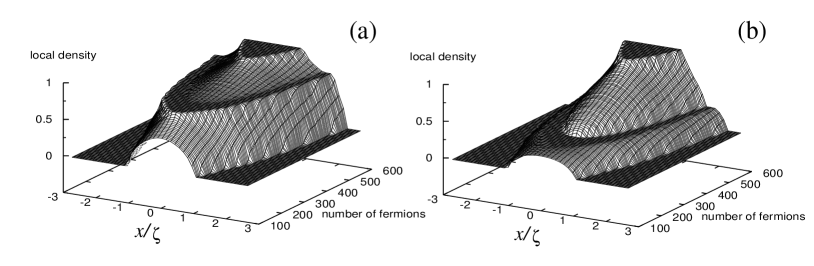
Figure 9: Evolution of the local density in a harmonic trap as a function of the position and increasing total number of fermions when an alternating potential $V_{a}=0.5t$ is present. (a) Odd sites. (b) Even sites. The system has 1000 lattice sites and $V_{2}a^{2}=3\times 10^{-5}t$.

In Figs. 10(a) and 10(b) we show the single particle spectrum and the level spacing respectively for the same parameters of Fig. 9. Although in this case the level spacing exhibits a more complicated structure, an immediate identification between the regions signaled in Fig. 10(b) between arrows and different fillings in Fig. 9 can be done. (A) corresponds to the fillings in Fig. 9 where only a metallic phase appears in the trap, (B) to the fillings where the first plateau is present in Fig. 9, (C) to the fillings where a metallic phase develops in the middle of the trap and it is surrounded by insulating regions, and (D) to the fillings in Fig. 9 where the insulator with $n=1$ appears in the center of the system. The region after the last arrow in Fig. 10(b) corresponds to deconfined states. Notice that the level spacing in regions (C) and (D) shows a behavior that was not present in Fig. 1.

Figure 10: Single particle spectrum (a) and level spacing (b) for a system with an alternating potential $V_{a}=0.5t$ and with $N=1000$ and $V_{2}a^{2}=3\times 10^{-5}t$. Energies are measured in units of $t$. For the explanation of the regions between the arrows, see text.

In order to understand the complex behavior of the level spacing we study, as in the previous section, the eigenfunctions of the system shown in Fig. 10. The eigenfunctions corresponding to region A in Fig. 1(b) behave as expected for a metallic phase, where the combination of the alternating and confining potentials generates a different modulation than the one studied in Sec. II, but without qualitative differences. In the second region of the spectrum (region B) the eigenfunctions have zero weight in the middle of the trap, exactly like in the insulator discussed in Sec. II. In region C there is, as pointed out above, a new feature since in this case it is possible to obtain a metallic region surrounded by an insulating one. This is reflected by the eigenfunctions shown in Fig. 11(a), where one of the eigenfunctions is nonzero only inside the local insulating phase (continuous line), and the other is nonzero only outside the insulating phase (dashed line), the energy levels associated with the latter ones are degenerated. For the region D the situation is similar but in this case the system is divided in four parts because of the existence of the insulator with $n=1$ in the middle of the trap and the insulator between the two metallic phases. This implies that all the levels are degenerate in region D, and the particles are located either between both insulating regions or outside the outermost one, as shown in Fig. 11(b).

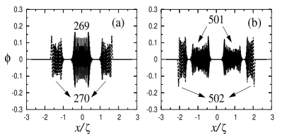
Figure 11: Eigenfunctions for a trapped system with an alternating potential ($V_{a}=0.5t$) for $N=1000$ and $V_{2}a^{2}=3\times 10^{-5}t$. The eigenfunctions correspond to the levels: 269 (a) (continuous line), 270 (a) (dashed line), 501 (b) (continuous line), and 502 (b) dashed line.

As in the previous section, the spectral features discussed here are equally valid for fermions as well as for bosons. Up to now we discussed the “slicing” of the systems only in terms of fermions and based on the appearance of insulating regions along the system. As before, it would be also here desirable to understand the appearance of forbidden regions in space in terms of a single particle picture. We show now that with the introduction of new Bragg conditions, due to the altered periodicity, the “slicing” of the system can be explained in an analogous way as in the previous section. In the unconfined case, the doubling of the periodicity creates new Bragg conditions at $k=\pm\pi/2a$, such that an energy gap $2V_{a}$ appears. Figure 10(a) shows that in the confined case the spectrum is continuous (in the sense that the level spacing is much smaller than $2V_{a}$), so that the imprint of the gap can be seen only in the local density of states

$$N_{i}(\omega)=\frac{1}{\pi}\mbox{Im}G_{ii}(\omega)\;,$$ (6)

where $G_{ij}(\omega)$ is the one-particle Green’s function mahan , which in this case can be easily computed.

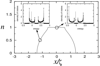
Figure 12: Density profile per unit cell (now containing two contiguous lattice sites) for a trap with $N=10000$, $V_{2}a^{2}=3\times 10^{-7}t$, and $N_{f}=2000$. The insets show the density of states per unit cell for two points in the profile. The arrows in the insets signal the Fermi energy for the selected filling.

The insets in Fig. 12 show the density of states per unit cell (now containing two lattice points) for two different positions along the density profile. The downward arrows in each inset corresponds to the location of the Fermi energy. The inset at the left corresponds to a situation where the Fermi energy goes through the lowest band, whereas the inset at the right belongs to sites in the middle of an insulating region. As expected, in this latter case, the Fermi energy lies inside the gap. The size of the gap is to a high degree of accuracy $2V_{a}$ for the site in the middle of the trap, but slightly less on the sides. Therefore, again the same arguments as before can be used, but instead of $4t$, the width for each band is given by $\sqrt{4t^{2}+V_{a}^{2}}-V_{a}\simeq 1.56t$ in our case. Without repeating the detailed discussion in the previous section, we can understand the confinement in Fig. 11(a) as follows. Level 269 has an energy that for sites in the middle of the trap falls in the middle of the upper band, while for level 270 (the same value of energy), passes through the lowest band. In fact, the density of states shown in Fig. 12 can be viewed as approximately shifted by $V_{2}x_{i}^{2}$, counting the sites from the middle. Finally, levels in Fig. 11(b) correspond to the case where in the middle of the trap they fall beyond the highest band, then going outwards, they fall in the middle of the highest band, and further outside, they fall in the middle of the lowest band.

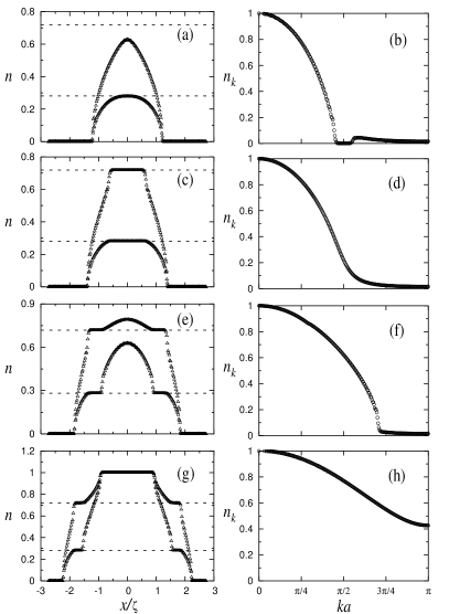
Figure 13: Density profiles (left) and their normalized MDF (right) for $N_{f}=150$ (a),(b), 200 (c),(d), 350 (e),(f), 600 (g),(h) and $N=1000$, $V_{a}=0.5t$, $V_{2}a^{2}=3\times 10^{-5}t$.

Again, as in Sec. II, one can follow the same reasoning by considering the MDF. Due to the new periodicity it displays new features, associated with the fact that increasing the periodicity the Brillouin zone is decreased, and in the present case a second Brillouin zone is visible. In Fig. 13 we show the density profiles (left) that characterize the four different situations present in Fig. 9. They correspond to fillings of the trap in the four regions of the single particle spectrum discussed previously in Fig. 10. Notice that in the figures we included all the odd and even points in the density profiles. We plotted as horizontal dashed lines the values of the densities in the band insulating phase of the periodic system for the odd and even sites (from top to bottom respectively), so that it can be seen where are located the local insulating phases in the trap. The corresponding normalized MDF are presented in Fig. 13 (right).

In Figs. 13(a) and 13(b) it is possible to see that when only the metallic phase is present in the trap, in the MDF an additional structure appears after $\pi/2$, corresponding to the contribution from the second Brillouin zone. When a first insulating phase is reached, by coming to the top of the lowest band, $k=\pi/2a$ is reached, and increasing the fillings of the system beyond that point, the dip around $k=\pi/2a$ disappears [Figs. 13(c) and 13(d)]. On adding more particles to the system a metallic phase appears inside the insulating plateau, [Figs. 13(e) and 13(f)]. When this metallic phase widens, decreasing the size of the insulating phase, $n_{k}$ starts to be similar to the $n_{k}$ of the pure metallic phase in the system without the alternating potential. Increasing even further the filling of the system, when the trivial insulator ($n=1$) appears in the center of the trap, the tail with very small values of $n_{k}$ disappears (like in the system without the alternating potential the region with $n_{k}$ zero also disappears [Fig. 3(b)] and the further increase of the filling in the system makes $n_{k}$ flatter [Figs. 13(h) and 13(i)].

Up to this point, several quantities, like density profile, pair distribution function, or local density of states were taken as evidence for the existence of an insulating phase, but a quantitative criterion in the sense of an order parameter to characterize the phases was not given. As shown already in the case of the Hubbard model rigol03_1 ; rigol03_2 , it is possible to define a local compressibility:

$$\kappa_{i}^{\ell}=\sum_{\mid j\mid\leq\,\ell(V_{a})}\chi_{i,i+j}\ ,$$ (7)

where

$$\chi_{i,j}=\left\langle n_{i}n_{j}\right\rangle-\left\langle n_{i}\right\rangle\left\langle n_{j}\right\rangle$$ (8)

is the density-density correlation function, and $\ell(V_{a})\simeq b\,\xi(V_{a})$, with $\xi(V_{a})$ the correlation length of $\chi_{i,j}$ in the periodic system at half-filling for the given value of $V_{a}$. As a consequence of the band gap opened in the band insulating phase at half filling in the periodic system, density-density correlations decay exponentially and there $\xi(V_{a})$ can be determined. The parameter $b$ is considered $b\sim 10$ (see discussion in Ref. rigol03_2 ). When this definition is applied to the different fillings of Fig. 9 the local compressibility is zero in the insulating regions and nonzero in the metallic phases. The local quantum critical behavior found in Ref. rigol03_1 at the transition between the metallic and Mott insulating phase is not present here since there are no interactions between the particles that could generate quantum criticality.

Finally we analyze the phase diagram for these systems. It can be generically described by the characteristic density $\tilde{\rho}$, like the Hubbard model and the noninteracting case in Sec. II. In Fig. 14 we show two phase diagrams for two different values of the curvature of the confining potential, $V_{2}a^{2}=3\times 10^{-5}t$ and $V_{2}a^{2}=3\times 10^{-4}t$. There it can be seen that although there is one order of magnitude between the curvatures of the confining potentials, the phase diagrams are one on top of the other, the small differences are only due to the finite number of particles which make the changes in $\tilde{\rho}$ discrete. Therefore, the characteristic density allows us to compare systems with different curvatures of the confining potential, number of particles and sizes. In addition we checked that keeping the characteristic density constant for a given value of $V_{a}$, the density profiles as a function of the normalized coordinates and the normalized MDF do not change when the number of particles or the curvature of the confining potential are changed in the system, as we already pointed out for the case without alternating potential (Sec. II).

Figure 14: Phase diagram for systems with $V_{2}a^{2}=3\times 10^{-5}t$ ($\bigtriangledown$) and $V_{2}a^{2}=3\times 10^{-4}t$ ($\bigcirc$). The different phases are explained in the text.

The different phases present in Fig. 14 are (A) a pure metallic phase, (B) an insulator in the middle of the trap surrounded by a metallic phase, (C) a metallic intrusion in the middle of the insulator, (D) an insulator with $n=1$ in the center of the trap surrounded by a metal, an insulator and the always present external metallic phase. For very small values of the alternating potential ($V_{a}$), phase B is not present, and the insulator surrounding the metallic phase in the center of the trap disappears leaving a full metallic phase at the very beginning of phase C. Similarly, the insulator with $n=1$ is surrounded only by a metallic phase (at the very beginning of phase D). However, these regions are very small in the phase diagram and we did not include them. At $V_{a}=0$ the results of Sec. II are recovered since up to $\tilde{\rho}=2.68$ the system is a pure metal and for higher characteristic densities there is an insulator with $n=1$ surrounded by metallic phases.

There is one important difference between the phase diagram in Fig. 14 and the one of the trapped Hubbard model rigol03_1 ; rigol03_2 . In Fig. 14 the boundary between regions A and B changes appreciably when the value on the alternating potential is increased while in the Hubbard model case (for the values of $U$ that we simulated) it was found independent of the value of $U$. This is possibly due to the fact that for the alternating potential, increasing $V_{a}$ changes the local densities of the insulating phase while in the local Mott insulating phase the density is always constant independently of the value of $U$.

V The 2D system

In this section we extend to 2D the results obtained in previous sections for the 1D case. The Hamiltonian in this case can be written as

$$H=-t\sum_{\langle i,j\rangle}\left(c^{\dagger}_{i}c_{j}+\text{H.c.}\right)+\sum_{i}\left(V_{\alpha_{x},x}\ x_{i}^{\alpha_{x}}+V_{\alpha_{y},y}y_{i}^{\alpha_{y}}\right)n_{i},$$ (9)

where ($x_{i},y_{i}$) are the coordinates of the site $i$, and $\langle i,j\rangle$ refers to nearest neighbors. The last term in Eq. (9) allows to consider different strengths $V_{\alpha_{x},x},\ V_{\alpha_{y},y}$ and powers $\alpha_{x},\ \alpha_{y}$ of the confining potential in the $x$, $y$ directions. We call in what follows $N_{x}$ and $N_{y}$ the number of lattice sites in the $x$ and $y$ directions, respectively.

In Fig. 15 we show the single particle spectrum and its corresponding level spacing for a system with $N_{x}=N_{y}=100$ lattice sites confined by a harmonic potential with $V_{2,x}a^{2}=V_{2,y}a^{2}=5\times 10^{-3}t$. Figure 15(b) shows that degeneracy sets in at the very beginning of the expectrum, and this is because of the symmetries of the square lattice. In 2D the formation of the insulator in the middle of the trap does not generate additional degeneracies in the system since it does not split the trap in independent identical parts. Then in contrast to the 1D case no information of its formation can be obtained from the level spacing.

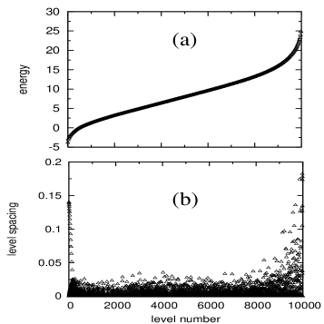
Figure 15: Single particle spectrum (a) and level spacing (b) for a system with $N_{x}=N_{y}=100$, and $V_{2,x}a^{2}=V_{2,y}a^{2}=5\times 10^{-3}t$. Energies are measured in units of $t$.

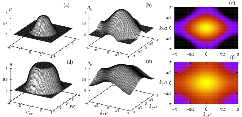
Figure 16: (Color online) 2D density profiles (a),(d), 2D normalized MDF (b),(e), and intensity plots of the 2D normalized MDF (c),(f), for $N_{f}=1000$ (a)–(c) and $N_{f}=4000$ (d)–(f) fermions in a system with $N_{x}=N_{y}=100$ and $V_{2,x}a^{2}=V_{2,y}a^{2}=5\times 10^{-3}t$. The color scale in (c) and (f) is the same as in Fig. 6.

Two density profiles and their corresponding normalized MDF for $N_{f}=1000$ and $N_{f}=4000$, and the same trap parameters of Fig. 15, are presented in Fig. 16. The $x$ and $y$ coordinates in the trap are normalized by the characteristic lengths $\zeta_{x}=\left(V_{2,x}/t\right)^{-1/2}$ and $\zeta_{y}=\left(V_{2,y}/t\right)^{-1/2}$, respectively. The density profile in Fig. 16(a) corresponds to a pure metallic phase in the 2D trap, the corresponding MDF [Fig. 16(b)] is smooth and for some momenta it is possible to see that $n_{k}=0$ like in the 1D case. When the filling of the system is increased, the insulator appears in the middle of the trap [Fig. 16(d)] and all the regions with $n_{k}=0$, present in the pure metallic phase, disappear from the MDF [Fig. 16(e)]. Figs. 16(c) and 16(f) show as intensity plots the normalized MDF of Figs. 16(b) and 16(e).

In 2D it is possible to define a dimensionless characteristic density as $\tilde{\rho}=N_{f}a^{2}/\zeta_{x}\zeta_{y}$. Also in this case it has always the same value when the insulator appears in the middle of the system, independently of the values and relations between $V_{2x}$ and $V_{2y}$. The density profiles as function of the normalized coordinates and the MDF remain unchanged when the characteristic density is kept constant and the values and relations between $V_{2x}$ and $V_{2y}$ are changed (in the thermodynamic limit they have the same form shown in Fig. 16). This implies that the results shown in Fig. 16 for a symmetric trap do not change for an asymmetric trap with the same characteristic density. The value of the characteristic density for the formation of the insulator in a harmonic 2D trap is $\tilde{\rho}_{C}\sim 13.5$.

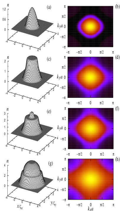
Figure 17: (Color online) Density per unit cell (a),(c),(e),(g) and intensity plots of the normalized MDF (b),(d),(f),(h) profiles for $N_{f}=200$ (a),(b), 800 (c),(d), 1100 (e),(f), and 3000 (h),(i) in a system with $N_{x}=N_{y}=100$, $V_{2,x}a^{2}=V_{2,y}a^{2}=5\times 10^{-3}t$, and $V_{a}=t$. The color scale in the intensity plots of the normalized MDF is the same as in Fig. 6.

The addition of the alternating potential leads to results similar to those presented in the 1D case. Four density profiles showing the possible local phases in the 2D trap, and intensity plots of their corresponding MDF are shown in Fig. 17. In the pure metallic case [Figs. 17(a) and 17(b)] the additional structure in the MDF for $k_{x},k_{y}>\pi/2a$, due to the increase of the periodicity, is present. This structure also disappears when the insulator appears in the middle of the system [Figs. 17(c) and 17(d)]. Increasing the filling a new metallic phase appears in the center of the trap [Figs. 17(c) and 17(d)]. For the highest filling the insulator with $n=1$ develops in the middle of the trap and the MDF becomes flatter with $n_{k}\neq 0$ everywhere. In a way similar to the 1D case there are confined states in the radial direction, i.e., particles are confined in rings around the center of the trap, and they can be explained in terms of Bragg conditions. The phase diagram of the 2D case is also similar to the one in the 1D case and is not discussed here.

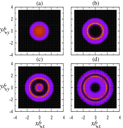
Figure 18: (Color online) Intensity plots of the local compressibility as a function of the normalized coordinates for systems with $N_{x}=N_{y}=100$, $V_{2,x}a^{2}=V_{2,y}a^{2}=5\times 10^{-3}t$ and $V_{a}=t$. The fillings are the same as that in Fig. 17 (a) $N_{f}=200$, (b) $N_{f}=800$, (c) $N_{f}=800$, and (d) $N_{f}=1100$. Black color means zero compressibility.

We close this section by considering the local compressibility. As it was mentioned in the analysis of the 1D case with the alternating potential, this quantity is zero in the insulating phases (like in the Mott insulating phases of the trapped Hubbard model). In the 2D case we extend the definition given by Eq. (7) to

$$\kappa_{i_{x}i_{y}}^{\ell}=\sum_{\mid j_{x},j_{y}\mid\leq\,\ell(V_{a})}\chi_{i_{x}i_{y},i_{x}+j_{x}i_{y}+j_{y}}\ ,$$ (10)

where

$$\chi_{i_{x}i_{y},j_{x}j_{y}}=\left\langle n_{i_{x}i_{y}}n_{j_{x}j_{y}}\right\rangle-\left\langle n_{i_{x}i_{y}}\right\rangle\left\langle n_{j_{x}j_{y}}\right\rangle,$$ (11)

is the density-density correlation function in 2D and $\ell(V_{a})\simeq b\,\xi(V_{a})$. In this case it is also possible to determine $\xi(V_{a})$ in the insulating phase of the 2D periodic case (at half filling) and apply the new definition to the 2D trap (as for the 1D case $b\sim 10$). The results obtained for the same parameters of Fig. 17 are presented in Fig. 18. There it can be seen that the rings of local insulators in Fig. 17 are represented in Fig. 18 by rings of incompressible regions (black rings) so that this definition works also perfectly in the 2D case, and the local compressibility should be a relevant quantity to characterize the local Mott insulating phases also in the trapped 2D Hubbard model.

VI Conclusions

We performed a detailed analysis of noninteracting systems focusing on the consequences of the combination of a confining and a periodic potential. It leads to a confinement of particles in a fraction of the available system size. This confinement is directly related to the formation of insulating regions in the case of fermionic systems. Since the results obtained correspond to noninteracting particles they can be also explained in a single particle picture due to the realization of Bragg conditions, and are also valid for bosons. We have studied the consequences of the previous confinement in the nonequilibrium dynamics of trapped particles in 1D when the center of the trap is suddenly displaced, and confirmed evolution of the center of mass obtained in recent experiments.

The region over which particles are confined in the trap can be controlled in various ways. The most obvious one is by changing the strength of the confining potential, where the extension of such regions can be regulated. Other way is changing the periodicity of the lattice, which leads to a different “slicing” of the system. The change of the periodicity also generates in the fermionic case the possibility of obtaining local insulating phases with sizes that can be controlled changing the strength of the additional alternating potential. This gives rise to a picture that is similar in some aspects to the the Hubbard model analyzed in Refs. rigol03_1 ; rigol03_2 . We have shown that although insulating phases appear in this noninteracting case, the gaps that are locally opened are not seen in the single particle spectrum. In order to observe them it is necessary to study the local density of states. The local compressibility defined in Refs. rigol03_1 ; rigol03_2 was also proven to be a genuine local order parameter to characterize the new insulating phases since it is always zero there. A scalable phase diagram for these systems was also presented. Finally, we considered the two-dimensional case and the formation of insulating regions due to the presence of periodic potentials. We showed that the local compressibility also characterizes those 2D regions in an unambiguous way.

- (1) M. H. Anderson, J. R. Ensher, M. R. Matthews, C. E. Wieman, and E. A. Cornell, Science 269, 198 (1995).
- (2) C. C. Bradley, C. A. Sackett, J. J. Tollett, and R. G. Hulet, Phys. Rev. Lett. 75, 1687 (1995).
- (3) K. B. Davis, M.-O. Mewes, M. R. Andrews, N. J. van Druten, D. S. Durfee, D. M. Kurn, and W. Ketterle, Phys. Rev. Lett. 75, 3969 (1995).
- (4) K. M. O’Hara, S. L. Hemmer, M. E. Gehm, S. R. Granade, and J. E. Thomas, Science 298, 2179 (2002).
- (5) F. Dalfovo, S. Giorgini, L. P. Pitaevskii, and S. Stringari, Rev. Mod. Phys. 71, 463 (1999).
- (6) F. Gleisberg, W. Wonneberger, U. Schlöder, and C. Zimmermann, Phys. Rev. A 62, 063602 (2000).
- (7) P. Vignolo, A. Minguzzi, and M. P. Tosi, Phys. Rev. Lett. 85, 2850 (2000).
- (8) A. Minguzzi, P. Vignolo, and M. P. Tosi, Phys. Rev. A 63, 063604 (2001) .
- (9) P. Vignolo, A. Minguzzi, and M. P. Tosi, Phys. Rev. A 64, 023421 (2001).
- (10) J. Schneider and H. Wallis, Phys. Rev. A 57, 1253 (1998).
- (11) M. Brack and B. P. van Zyl, Phys. Rev. Lett. 86, 1574 (2001).
- (12) P. Vignolo and A. Minguzzi, Phys. Rev. A 67, 053601 (2003).
- (13) M. Greiner, O. Mandel, T. Esslinger, T. W. Hänsch, and I. Bloch, Nature (London) 415, 39 (2002).
- (14) W. Hofstetter, J. I. Cirac, P. Zoller, E. Demler, and M. D. Lukin, Phys. Rev. Lett. 89, 220407 (2002).
- (15) G. Modugno, F. Ferlaino, R. Heidemann, G. Roati, and M. Inguscio, Phys. Rev. A 68, 011601(R) (2003).
- (16) H. Ott, E. de Mirandes, F. Ferlaino, G. Roati, G. Modugno, and M. Inguscio, Phys. Rev. Lett. 92, 160601 (2004).
- (17) L. Pezze’, L. Pitaevskii, A. Smerzi, S. Stringari, G. Modugno, E. de Mirandes, F. Ferlaino, H. Ott, G. Roati, and M. Inguscio, Phys. Rev. Lett. 93, 120401 (2004).
- (18) T. A. B. Kennedy, Phys. Rev. A 70, 023603 (2004).
- (19) V. Ruuska and P. Törmä, New J. Phys. 6, 59 (2004).
- (20) M. Rigol, A. Muramatsu, G. G. Batrouni, and R. T. Scalettar, Phys. Rev. Lett. 91, 130403 (2003).
- (21) M. Rigol and A. Muramatsu, Phys. Rev. A 69, 053612 (2004).
- (22) G. G. Batrouni, V. Rousseau, R. T. Scalettar, M. Rigol, A. Muramatsu, P. J. H. Denteneer and M. Troyer, Phys. Rev. Lett. 89, 117203 (2002).
- (23) W. Zwerger, J. Opt. B: Quantum Semiclassical Opt. 5, S9 (2003).
- (24) We thank T. Pfau for suggesting the line of thinking displayed below.
- (25) C. Zener, Proc. R. Soc. London, Ser. A 145, 523 (1934).
- (26) V. A. Kashurnikov, N. V. Prokof’ev, and B. V. Svistunov, Phys. Rev. A 66, 031601(R) (2002).
- (27) G. D. Mahan, Many-Particle Physics (Plenum, New York and London, 1986).