Group expansions for impurities in superconductors

Abstract

A new method is proposed for practical calculation of the effective interaction between impurity scatterers in superconductors, based on algebraic properties of related Nambu matrices for Green functions. In particular, we show that the density of states within the s-wave gap can have a non-zero contribution (impossible either in Born and in T-matrix approximation) from non-magnetic impurities with concentration $c\ll 1$, beginning from $\sim c^{3}$ order.

I introduction

Impurity effects are at the center of interest in studies of superconducting (SC) materials, especially of those with high transition temperature (HTSC). In the general theory of disordered systems with disorder due to diluted impurity centers, the so-called group expansion (GE) method was proposed as most consistent for quasiparticle Green function (GF) iv , and it was also formulated for SC systems pog .

The GE’s of different types (see below) are analogous to the classical Ursell-Mayer group series in the theory of non-ideal gases may , where the particular terms (the group integrals) include physical interactions in groups of the given number of particles. In the quantum theory of solids, GE includes indirect interactions (dependent on the excitation energy $\varepsilon$) between the impurity centers, through the exchange by virtual excitations from (admittedly renormalized) band spectrum, so that each term corresponds to summation of certain infinite series of diagrams. These expansions were elaborated in a detail for various kinds of normal quasiparticle spectra, where they define the interplay between extended and localized states ilp , however their usage in SC systems encounters considerable technical difficulties due to existence of anomalous GF’s.

The present paper is aimed on an efficient algorithm for resolving these difficulties. We develop the specific algebraic techniques to calculate Nambu matrices in various terms of GE for the exemplary case of s-wave symmetry of SC order parameter, permitting to explore the impurity effects in this case beyond the scope of Anderson theorem and . In particular, we find that pair clusters of impurities (2nd term of GE) can not produce finite contribution into the quasiparticle density of states (DOS) within the s-wave gap, alike the simplest effect of isolated impurities (1st GE term), but a non-zero contribution into the in-gap DOS is already possible for the 3rd GE term (impurity triples). These results allow also a straightforward extension to the d-wave symmetry characteristic for doped HTSC materials (where the dopants not only supply the charge carriers but also play the role of impurity scatterers).

II Hamiltonian and Green functions

For description of electronic spectra in a SC system with impurities, it is convenient to use the formalism of Nambu spinors: the row-spinor $\psi_{\mathbf{k}}^{\dagger}=(a_{\mathbf{k},\uparrow}^{\dagger},a_{-\mathbf{k},\downarrow})$ and respective column-spinor $\psi_{\mathbf{k}}$, writing the Hamiltonian in a spinor form

$$H_{sc}=\sum_{\mathbf{k}}[\psi_{\mathbf{k}}^{\dagger}(\xi_{\mathbf{k}}\widehat{\tau}_{3}+\Delta_{\mathbf{k}}\widehat{\tau}_{1})\psi_{\mathbf{k}}-\frac{1}{N}\sum_{\mathbf{p},\mathbf{k}^{\prime}}\mathrm{e}^{i(\mathbf{k}-\mathbf{k}^{\prime})\mathbf{p}}\psi_{\mathbf{k}^{\prime}}^{\dagger}\widehat{V}\psi_{\mathbf{k}}].$$ (1)

It includes the normal quasiparticle energy $\xi_{\mathbf{k}}$, the mean-field gap function $\Delta_{\mathbf{k}}$, the Pauli matrices $\widehat{\tau}_{j}$ and the perturbation matrix $\widehat{V}=V_{\mathrm{L}}\widehat{\tau}_{3}$. The impurity (attractive) perturbation on random sites $\mathbf{p}$ with concentration $c=\sum_{\mathbf{p}}1/N\ll 1$ is described by the Lifshitz parameter $V_{\mathrm{L}}$.

The energy spectrum of a Fermi system is described through the Fourier transformed two-time Green functions (GF’s) eco :

$$\langle\langle a|b\rangle\rangle_{\varepsilon}=i\int_{-\infty}^{0}{\textrm{e}}^{i(\varepsilon-i0)t}\langle\{a(t),b(0)\}\rangle dt,$$ (2)

where $\langle\ldots\rangle$ is the quantum statistical average and $\{.,.\}$ is the anticommutator of operators in Heisenberg representation. For the system, Eq. 1, we define the $2\times 2$ Nambu matrix of GF’s

$$\widehat{G}_{\mathbf{k},\mathbf{k}^{\prime}}=\langle\langle\psi_{\mathbf{k}}|\psi_{\mathbf{k}^{\prime}}^{\dagger}\rangle\rangle.$$ (3)

The matrix elements in the expanded form of Eq. 3 are the well-known Gor’kov normal and anomalous functions gor . In what follows, we shall also distinguish between the Nambu indices (N-indices) and the quasi-momentum indices (m-indices) in this matrix. In absence of impurities, the explicit form of the matrix, Eq. 3, turns: $\widehat{G}_{\mathbf{k},\mathbf{k}^{\prime}}\rightarrow\delta_{\mathbf{k},\mathbf{k}^{\prime}}\widehat{G}_{\mathbf{k}}^{0}$, where the non-perturbed (m-diagonal) GF matrix

$$\widehat{G}_{\mathbf{k}}^{0}=\frac{\varepsilon+\xi_{\mathbf{k}}\widehat{\tau}_{3}+\Delta_{\mathbf{k}}\widehat{\tau}_{1}}{\varepsilon^{2}-E_{\mathbf{k}}^{2}}$$ (4)

involves the SC quasiparticle energy $E_{\mathbf{k}}=\sqrt{\xi_{\mathbf{k}}^{2}+\Delta_{\mathbf{k}}^{2}}$. The relevant physical properties of SC state are suitably expressed in terms of these GF’s. For instance, the single-particle DOS, related to the electronic specific heat, is given by

$$\rho(\varepsilon)=\frac{1}{\pi N}\sum_{\mathbf{k}}\mathrm{Tr}\>{\textrm{Im}}\widehat{G}_{\mathbf{k}}$$ (5)

where $\widehat{G}_{\mathbf{k}}\equiv\widehat{G}_{\mathbf{k},\mathbf{k}}$ is the m-diagonal GF.

Now we pass to calculation of GF’s in SC systems at finite concentration $c$ of impurity centers and analyze explicit structure of corresponding GE’s.

III Group expansions for self-energy

We derive GE’s for the system defined by the Hamiltonian Eq. 1, starting from the Dyson equation of motion for a matrix GF:

$$\widehat{G}_{\mathbf{k},\mathbf{k}^{\prime}}=\widehat{G}_{\mathbf{k}}^{0}\delta_{\mathbf{k},\mathbf{k}^{\prime}}-\frac{1}{N}\sum_{\mathbf{p},\mathbf{k}^{\prime\prime}}\mathrm{e}^{i(\mathbf{\mathbf{k}^{\prime\prime}}-\mathbf{k}^{\prime})\mathbf{p}}\widehat{G}_{\mathbf{k}}^{0}\widehat{V}\widehat{G}_{\mathbf{k}^{\prime\prime},\mathbf{k}^{\prime}}.$$ (6)

A routine consists in consecutive iterations of the same equations for the GF’s in the “scattering” terms of Eq. 6 and separating systematically those already present in the previous iterations iv . Thus, for the m-diagonal GF $\widehat{G}_{\mathbf{k}}$, we first separate the scattering term with the function $\widehat{G}_{\mathbf{k}}$ itself from those with $\widehat{G}_{\mathbf{k}^{\prime},\mathbf{k}}$, $\mathbf{k}^{\prime}\neq\mathbf{k}$:

$$\widehat{G}_{\mathbf{k}}=\widehat{G}_{\mathbf{k}}^{0}-\frac{1}{N}\sum_{\mathbf{k}^{\prime},\mathbf{p}}\mathrm{e}^{i\left(\mathbf{k}-\mathbf{k}^{\prime}\right)\cdot\mathbf{p}}\widehat{G}_{\mathbf{k}}^{0}\widehat{V}\widehat{G}_{\mathbf{k}^{\prime},\mathbf{k}}=$$

$$=\widehat{G}_{\mathbf{k}}^{0}-c\widehat{G}_{\mathbf{k}}^{0}\widehat{V}\widehat{G}_{\mathbf{k}}-\frac{1}{N}\sum_{\mathbf{k}^{\prime}\neq\mathbf{k},\mathbf{p}}\mathrm{e}^{i\left(\mathbf{k}-\mathbf{k}^{\prime}\right)\cdot\mathbf{p}}\widehat{G}_{\mathbf{k}}^{0}\widehat{V}\widehat{G}_{\mathbf{k}^{\prime},\mathbf{k}}.$$ (7)

Then for each $\widehat{G}_{\mathbf{k}^{\prime},\mathbf{k}}$, $\mathbf{k}^{\prime}\neq\mathbf{k}$ we write down Eq. 6 again and single out the scattering terms with $\widehat{G}_{\mathbf{k}}$ and $\widehat{G}_{\mathbf{k}^{\prime},\mathbf{k}}$ in its r.h.s:

$$\widehat{G}_{\mathbf{k}^{\prime},\mathbf{k}}=-\frac{1}{N}\sum_{\mathbf{k}^{\prime\prime},\mathbf{p}^{\prime}}\mathrm{e}^{i\left(\mathbf{k}^{\prime}-\mathbf{k}^{\prime\prime}\right)\cdot\mathbf{p}}\widehat{G}_{\mathbf{k}^{\prime}}^{0}\widehat{V}\widehat{G}_{\mathbf{k}^{\prime\prime},\mathbf{k}}=$$

$$=-c\widehat{G}_{\mathbf{k}^{\prime}}^{0}\widehat{V}\widehat{G}_{\mathbf{k}^{\prime},\mathbf{k}}-\frac{1}{N}\mathrm{e}^{i\left(\mathbf{k}^{\prime}-\mathbf{k}\right)\cdot\mathbf{p}}\widehat{G}_{\mathbf{k}^{\prime}}^{0}\widehat{V}\widehat{G}_{\mathbf{k}}$$

$$-\frac{1}{N}\sum_{\mathbf{p^{\prime}\neq p}}\mathrm{e}^{i\left(\mathbf{k}^{\prime}-\mathbf{k}\right)\cdot\mathbf{p}^{\prime}}\widehat{G}_{\mathbf{k}^{\prime}}^{0}\widehat{V}\widehat{G}_{\mathbf{k}}$$

$$-\frac{1}{N}\sum_{\mathbf{k}^{\prime\prime}\neq\mathbf{k},\mathbf{k}^{\prime};\mathbf{p}^{\prime}}\mathrm{e}^{i\left(\mathbf{k}^{\prime}-\mathbf{k}^{\prime\prime}\right)\cdot\mathbf{p}^{\prime}}\widehat{G}_{\mathbf{k}^{\prime}}^{0}\widehat{V}\widehat{G}_{\mathbf{k}^{\prime\prime},\mathbf{k}}.$$ (8)

Note that among the terms with $\widehat{G}_{\mathbf{k}}$, the $\mathbf{p}^{\prime}=\mathbf{p}$ term (the second in r.h.s. of Eq. 8) bears the phase factor $\mathrm{e}^{i\left(\mathbf{k}^{\prime}-\mathbf{k}\right)\cdot\mathbf{p}}$, so it is coherent to that already figured in the last sum in Eq. 7. That is why this term is explicitly separated from other, incoherent ones, $\mathrm{\propto e}^{i\left(\mathbf{k}^{\prime}-\mathbf{k}\right)\cdot\mathbf{p}^{\prime}}$, $\mathbf{p}^{\prime}\neq\mathbf{p}$ (but there will be no such separation when doing 1st iteration of Eq. 6 for the m-non-diagonal GF $\widehat{G}_{\mathbf{k}^{\prime\prime},\mathbf{k}}$ itself).

Continuing the sequence, we collect the terms with the initial function $\widehat{G}_{\mathbf{k}}$which result from: i) all multiple scatterings on the same site $\mathbf{p}$ and ii) such processes on the same pair of sites $\mathbf{p}$ and $\mathbf{p}^{\prime}\neq\mathbf{p}$. Then summation in $\mathbf{p}$ of the i)-terms gives rise to the first term of GE, and, if the pair processes were neglected, it would coincide with the well known result of self-consistent T-matrix approximation baym . The second term of GE, obtained by summation in $\mathbf{p},\mathbf{p}^{\prime}\neq\mathbf{p}$ of the ii)-terms, contains certain interaction matrices $\widehat{A}_{\mathbf{p}^{\prime},\mathbf{p}}$ generated by the multiply scattered functions $\widehat{G}_{\mathbf{k}^{\prime},\mathbf{k}}$, $\mathbf{k}^{\prime}\neq\mathbf{k}$, etc., (including their own renormalization). For instance, the iterated equation of motion for a function $\widehat{G}_{\mathbf{k}^{\prime\prime},\mathbf{k}}$ with $\mathbf{k}^{\prime\prime}\neq\mathbf{k},\mathbf{k}^{\prime}$ in the last term of Eq. 7 will produce:

$$\widehat{G}_{\mathbf{k}^{\prime\prime},\mathbf{k}}=-\frac{1}{N}\sum_{\mathbf{k}^{\prime\prime\prime},\mathbf{p}^{\prime\prime}}\mathrm{e}^{i\left(\mathbf{k}^{\prime\prime}-\mathbf{k}^{\prime\prime\prime}\right)\cdot\mathbf{p}^{\prime\prime}}\widehat{G}_{\mathbf{k}^{\prime\prime}}^{0}\widehat{V}\widehat{G}_{\mathbf{k}^{\prime\prime\prime},\mathbf{k}}=$$

$$=-\frac{\mathrm{e}^{i\left(\mathbf{k}^{\prime\prime}-\mathbf{k}\right)\cdot\mathbf{p}}}{N}\widehat{G}_{\mathbf{k}^{\prime\prime}}^{0}\widehat{V}\widehat{G}_{\mathbf{k}}-\frac{\mathrm{e}^{i\left(\mathbf{k}^{\prime\prime}-\mathbf{k}\right)\cdot\mathbf{p}^{\prime}}}{N}\widehat{G}_{\mathbf{k}^{\prime\prime}}^{0}\widehat{V}\widehat{G}_{\mathbf{k}}+$$

$$+\quad\mathrm{terms\quad with}\quad\widehat{G}_{\mathbf{k}^{\prime},\mathbf{k}}\quad\mathrm{and}\quad\widehat{G}_{\mathbf{k}^{\prime\prime},\mathbf{k}}+$$

$$+\quad\mathrm{terms\quad with}\quad\widehat{G}_{\mathbf{k}^{\prime\prime\prime},\mathbf{k}}\;(\mathbf{k}^{\prime\prime\prime}\neq\mathbf{k},\mathbf{k}^{\prime},\mathbf{k}^{\prime\prime}).$$ (9)

Consequently, we obtain the solution for an m-diagonal GF as

$$\widehat{G}_{\mathbf{k}}=\widehat{G}_{\mathbf{k},\mathbf{k}}=\left[\left(\widehat{G}_{\mathbf{k}}^{0}\right)^{-1}-\widehat{\Sigma}_{\mathbf{k}}\right]^{-1},$$ (10)

with the matrix GE for the renormalized self-energy matrix:

$$\widehat{\Sigma}_{\mathbf{k}}=c\widehat{T}\left[1+c\sum_{\mathbf{n}\neq 0}\left(\widehat{A}_{0,\mathbf{n}}{\textrm{e}}^{-i\mathbf{kn}}+\widehat{A}_{0,\mathbf{n}}\widehat{A}_{\mathbf{n},0}\right)\times\right.$$

$$\left.\times\left(1-\widehat{A}_{0,\mathbf{n}}\widehat{A}_{\mathbf{n},0}\right)^{-1}+\cdots\right].$$ (11)

Here $\widehat{T}=-\widehat{V}\left(1+\widehat{G}\widehat{V}\right)^{-1}$ is the renormalized T-matrix, and the indirect interaction (mediated by the quasiparticles of host crystal) between two impurities at lattice sites $0$ and $\mathbf{n}$ is described by the matrix $\widehat{A}_{0,\mathbf{n}}=N^{-1}\sum_{\mathbf{k}^{\prime}\neq\mathbf{k}}{\textrm{e}}^{i\mathbf{\mathbf{k}^{\prime}n}}\widehat{G}_{\mathbf{k}^{\prime}}\widehat{T}$, with the sum in quasi-momenta restricted due to the above algorithm of separation. There are even more such restrictions in each product of these matrices: $\widehat{A}_{0,\mathbf{n}}\widehat{A}_{\mathbf{n},0}=N^{-2}\sum_{\mathbf{k}^{\prime}\neq\mathbf{k}}\sum_{\mathbf{k}^{\prime\prime}\neq\mathbf{k},\mathbf{k}^{\prime}}{\textrm{e}}^{i\mathbf{\left(\mathbf{k}^{\prime}-\mathbf{k}^{\prime\prime}\right)n}}\widehat{G}_{\mathbf{k}^{\prime}}\widehat{T}\widehat{G}_{\mathbf{k}^{\prime\prime}}\widehat{T}$, and so on. This seems to seriously hamper calculation of the sum $\sum_{\mathbf{n}\neq 0}$ in Eq. 11 (not to say about higher GE terms). However, the difficulty is avoided, taking into account the identities for two first terms of its expansion iv :

$$\sum_{\mathbf{n}\neq 0}\widehat{A}_{0,\mathbf{n}}{\textrm{e}}^{-i\mathbf{kn}}=-\widehat{A}_{0,0}+\sum_{\mathbf{n}}\widehat{A}_{0,\mathbf{n}}{\textrm{e}}^{-i\mathbf{kn}}=$$

$$=-\widehat{A}_{0,0}+\frac{1}{N}\sum_{\mathbf{n}}\sum_{\mathbf{k}^{\prime}\neq\mathbf{k}}{\textrm{e}}^{i\mathbf{\left(\mathbf{k}^{\prime}-\mathbf{k}\right)n}}\widehat{G}_{\mathbf{k^{\prime}}}\widehat{T}=$$

$$=-\widehat{A}_{0,0},$$

and

$$\sum_{\mathbf{n}\neq 0}\widehat{A}_{0,\mathbf{n}}\widehat{A}_{\mathbf{n},0}=-\widehat{A}_{0,0}^{2}+\sum_{\mathbf{n}}\widehat{A}_{0,\mathbf{n}}\widehat{A}_{\mathbf{n},0}=-\widehat{A}_{0,0}^{2}+$$

$$+\frac{1}{N^{2}}\sum_{\mathbf{n}}\sum_{\mathbf{k}^{\prime},\mathbf{k}^{\prime\prime}\neq\mathbf{k}^{\prime}}{\textrm{e}}^{i\mathbf{\left(\mathbf{k}^{\prime}-\mathbf{k}^{\prime\prime}\right)n}}\widehat{G}_{\mathbf{k^{\prime}}}\widehat{T}\widehat{G}_{\mathbf{k}^{\prime\prime}}\widehat{T}=$$

$$=-\widehat{A}_{0,0}^{2},$$

due to the momentum independence of T-matrix, and the fact that the restrictions can be simply ignored in the higher products, like

$$\sum_{\mathbf{n}\neq 0}\widehat{A}_{0,\mathbf{n}}\widehat{A}_{\mathbf{n},0}\widehat{A}_{0,\mathbf{n}}{\textrm{e}}^{-i\mathbf{kn}}=-\widehat{A}_{0,0}^{3}+$$

$$+\sum_{\mathbf{n}}\widehat{A}_{0,\mathbf{n}}\widehat{A}_{\mathbf{n},0}\widehat{A}_{0,\mathbf{n}}{\textrm{e}}^{-i\mathbf{kn}}=-\widehat{A}_{0,0}^{3}+$$

$$\frac{1}{N^{3}}\sum_{\mathbf{n}}\sum_{\mathbf{k}^{\prime},\mathbf{k}^{\prime\prime}\neq\mathbf{k}^{\prime}}{\textrm{e}}^{i\mathbf{\left(\mathbf{k}^{\prime}-\mathbf{k}^{\prime\prime}+\mathbf{k}^{\prime\prime\prime}-\mathbf{k}\right)n}}\widehat{G}_{\mathbf{k^{\prime}}}\widehat{T}\widehat{G}_{\mathbf{k}^{\prime\prime}}\widehat{T}\widehat{G}_{\mathbf{k}^{\prime\prime\prime}}\widehat{T}=$$

$$-\widehat{A}_{0,0}^{3}+\frac{1}{N^{2}}\sum_{\mathbf{k}^{\prime},\mathbf{k}^{\prime\prime}}\widehat{G}_{\mathbf{k^{\prime}}}\widehat{T}\widehat{G}_{\mathbf{k}^{\prime\prime}}\widehat{T}\widehat{G}_{\mathbf{k}-\mathbf{k^{\prime}}+\mathbf{k}^{\prime\prime}}\widehat{T},$$

etc. Thus we arrive at the final form for the renormalized GE

$$\widehat{\Sigma}_{\mathbf{k}}=c\widehat{T}\left[1-c\widehat{A}_{0,0}-c\widehat{A}_{0,0}^{2}+\right.$$

$$\left.+c\sum_{\mathbf{n}\neq 0}\left(\widehat{A}_{0,\mathbf{n}}^{3}{\textrm{e}}^{-i\mathbf{kn}}+\widehat{A}_{0,\mathbf{n}}^{4}\right)\left(1-\widehat{A}_{0,\mathbf{n}}^{2}\right)^{-1}+\cdots\right]$$ (12)

where $\widehat{A}_{0,\mathbf{n}}=\widehat{G}_{0,\mathbf{n}}\widehat{T}$ and the renormalized local GF matrices $\widehat{G}_{0,\mathbf{n}}=N^{-1}\sum_{\mathbf{k}}{\textrm{e}}^{i\mathbf{kn}}\widehat{G}_{\mathbf{k}}$ and $\widehat{G}=\widehat{G}_{0,0}$ are already free from restrictions. The two terms, next to unity in the brackets in Eq. 12, correspond to the excluded double occupancy of the same site by impurities, the sum in $\mathbf{n}\neq 0$ describes the averaged contribution of all possible impurity pairs, and the dropped terms are for triples and more of impurities.

An alternative routine for Eq. 6 consists in its iteration for all the terms $\widehat{G}_{\mathbf{k}^{\prime\prime},\mathbf{k}}$ and summing the contributions $\propto\widehat{G}_{\mathbf{k}}^{0}$, like the first term in r.h.s. of Eq. 6. This finally leads to the solution of form

$$\widehat{G}_{\mathbf{k}}=\widehat{G}_{\mathbf{k}}^{0}+\widehat{G}_{\mathbf{k}}^{0}\widehat{\Sigma}_{\mathbf{k}}^{0}\widehat{G}_{\mathbf{k}}^{0},$$ (13)

with the non-renormalized self-energy matrix

$$\widehat{\Sigma}_{\mathbf{k}}^{0}=c\widehat{T}^{0}\left\{1+c\sum_{\mathbf{n}\neq 0}\left[\widehat{A}_{0,\mathbf{n}}^{0}{\textrm{e}}^{-i\mathbf{kn}}+\left(\widehat{A}_{0,\mathbf{n}}^{0}\right)^{2}\right]\times\right.$$

$$\left.\times\left[1-\left(\widehat{A}_{0,\mathbf{n}}^{0}\right)^{2}\right]^{-1}+\cdots\right\},$$ (14)

and the respective elements $\widehat{T}^{0}=-\widehat{V}\left(1+\widehat{G}^{0}\widehat{V}\right)^{-1}$, $\widehat{A}_{0,\mathbf{n}}^{0}=\widehat{G}_{0,\mathbf{n}}^{0}\widehat{T}^{0}$, $\widehat{G}_{0,\mathbf{n}}^{0}=N^{-1}\sum_{\mathbf{k}}{\textrm{e}}^{i\mathbf{kn}}\widehat{G}_{\mathbf{k}}^{0}$ and $\widehat{G}^{0}=\widehat{G}_{0,0}^{0}$.

Presenting GF’s in the disordered system in the form of GE’s generally leads to respective expansions for its observable characteristics. For instance, the impurity perturbed DOS is expected in the form: $\rho\left(\varepsilon\right)=\rho_{0}\left(\varepsilon\right)+\rho_{1}\left(\varepsilon\right)+\rho_{2}\left(\varepsilon\right)+\ldots$, related to contributions of pure crystal, isolated impurities, impurity pairs, etc.

However, usage of each type of GE, the renormalized Eq. 12 or the non-renormalized Eq. 14, is only justified if they are convergent (at least, asymptotically). Since the matrices $\widehat{T}$ and $\widehat{A}$ are energy dependent, convergence of each type of GE is restricted to certain energy ranges, and these ranges are generally different. For a number of normal systems with impurities, where GE’s are constructed of scalar functions $A_{0,\mathbf{n}}$, it was shown that the renormalized GE converges within the region of band-like states, well characterized by the wave-vector, and the non-renormalized GE does within the region of localized states ilp . To get quantitative estimates of convergence and higher order contributions to self-energy, operating with the matrix functions $\widehat{A}_{0,\mathbf{n}}$ in Eqs. 12 and 14, a special techniques is necessary that we construct below.

IV Algebraic techniques for Nambu matrices

Let us explicitly calculate the elements of above defined GE’s for the simplest s-wave symmetry of the SC gap function: $\Delta_{s}\left(\mathbf{k}\right)=\Delta$. The unperturbed local GF matrix is obtained as an expansion in Pauli matrices:

$$\widehat{G}^{0}=-\left(\varepsilon+\Delta\widehat{\tau}_{1}\right)g_{0}-g_{3}\widehat{\tau}_{3},$$ (15)

where

$$g_{0}\left(\varepsilon\right)=\frac{\pi\rho_{{\textrm{F}}}}{2\sqrt{\Delta^{2}-\varepsilon^{2}}},$$

defines the s-wave DOS in pure crystal: $\rho_{0}\left(\varepsilon\right)=(2/\pi){\textrm{Im}}g_{0}\left(\varepsilon\right)$ (with the Fermi DOS $\rho_{{\textrm{F}}}$ of normal quasiparticles), and the electron-hole asymmetry factor

$$g_{3}\left(\varepsilon\right)=\frac{1}{N}\sum_{\mathbf{k}}\frac{\xi_{\mathbf{k}}}{E_{\mathbf{k}}^{2}-\varepsilon^{2}}\approx\frac{1}{N}\sum_{\mathbf{k}}\frac{\xi_{\mathbf{k}}}{E_{\mathbf{k}}^{2}}\sim\rho_{{\textrm{F}}},$$

is almost constant and real.

Then we readily calculate the non-renormalized T-matrix:

$$\widehat{T}^{0}=\frac{2}{\pi\rho_{{\textrm{F}}}}\frac{v}{1+v^{2}}\left(\widehat{\tau}_{3}+v\frac{\varepsilon-\Delta\widehat{\tau}_{1}}{\sqrt{\Delta^{2}-\varepsilon^{2}}}\right),$$ (16)

with the dimensionless perturbation parameter

$$v=\frac{\pi}{2}\frac{V_{\mathrm{L}}\rho_{{\textrm{F}}}}{1-V_{\mathrm{L}}g_{3}}.$$

Since the denominator $1+v^{2}$ in Eq. 16 can not be zero, the quasiparticle localization on a single impurity center in the considered s-wave superconductor turns impossible pog . If the self-energy is approximated by the first term of GE: $\widehat{\Sigma}_{\mathbf{k}}\approx c\widehat{T}^{0}$, then Eq. 16 used in Eq. 13 and in Eq. 5 leads to the same DOS $\rho_{0}\left(\varepsilon\right)$ (that is, $\rho_{1}\left(\varepsilon\right)\equiv 0$) with the same gap value $\Delta$ as in pure crystal. This justifies Anderson’s theorem and within T-matrix approximation for an s-wave SC with point-like impurity perturbations.

However, even if there is no in-gap poles in the single-impurity T-matrix term, they can appear in the following terms of GE, that would describe localized states on impurity clusters ilp . Thus, the pair contribution:

$$\rho_{2}\left(\varepsilon\right)=\frac{c^{2}}{\pi N}\sum_{\mathbf{k},\mathbf{n}\neq 0}\mathrm{Tr\>Im}\widehat{G}_{\mathbf{k}}^{0}\widehat{T}^{0}\left[\widehat{A}_{0,\mathbf{n}}^{0}\cos\mathbf{kn}+\left(\widehat{A}_{0,\mathbf{n}}^{0}\right)^{2}\right]\times$$

$$\times\left[1-\left(\widehat{A}_{0,\mathbf{n}}^{0}\right)^{2}\right]^{-1}\widehat{G}_{\mathbf{k}}^{0}\widehat{\tau}_{3},$$ (17)

should only follow from the poles of $[1-(\widehat{A}_{0,\mathbf{n}}^{0})^{2}]^{-1}$, since the matrix $\widehat{A}_{0,\mathbf{n}}^{0}\left(\varepsilon\right)$ is real at $\varepsilon^{2}<$ $\Delta^{2}$.

In fact, the long distance asymptotics of this matrix (at $n\gg a$) is:

$$\widehat{A}_{0,\mathbf{n}}^{0}\approx-\mathcal{F}_{0,\mathbf{n}}\left(\varepsilon\right)\left(\cos\varphi_{\mathbf{n}}+\frac{\varepsilon\widehat{\tau}_{3}-i\Delta\widehat{\tau}_{2}}{\sqrt{\Delta^{2}-\varepsilon^{2}}}\sin\varphi_{\mathbf{n}}\right),$$ (18)

where $\varphi_{\mathbf{n}}=k_{\mathrm{F}}\left|\mathbf{n}\right|+\delta$ and the particular forms for the scalar “envelop” function $\mathcal{F}_{0,\mathbf{n}}\left(\varepsilon\right)$ and the phase shift $\delta$ depend on the system dimensionality:

$$\mathcal{F}_{0,\mathbf{n}}\left(\varepsilon\right)=\frac{v}{\sqrt{1+v^{2}}}\frac{\sqrt{2}{\textrm{e}}^{-\left|\mathbf{n}\right|/r_{\varepsilon}}}{\sqrt{\pi k_{\mathrm{F}}\left|\mathbf{n}\right|}},\quad\cot\delta=\frac{1-v}{1+v},$$ (19)

for 2D, and

$$\mathcal{F}_{0,\mathbf{n}}\left(\varepsilon\right)=\frac{v}{\sqrt{1+v^{2}}}\frac{{\textrm{e}}^{-\left|\mathbf{n}\right|/r_{\varepsilon}}}{k_{\mathrm{F}}\left|\mathbf{n}\right|},\quad\cot\delta=1/v,$$ (20)

for 3D, with the energy dependent decay length $r_{\varepsilon}=a^{2}k_{\mathrm{F}}/(\pi\rho_{0}\sqrt{\Delta^{2}-\varepsilon^{2}})$.

The following analysis is essentially simplified, introducing matrices of the structure:

$$\widehat{M}(a,b)=a+b\frac{\varepsilon\widehat{\tau}_{3}-i\Delta\widehat{\tau}_{2}}{\sqrt{\Delta^{2}-\varepsilon^{2}}},$$ (21)

which form a closed algebra with the product rule for the $a,b$ components:

$$\widehat{M}\left(a,b\right)\widehat{M}\left(a^{\prime},b^{\prime}\right)=\widehat{M}\left(aa^{\prime}-bb^{\prime},ab^{\prime}+ba^{\prime}\right).$$ (22)

In this notation, the interaction matrices, Eq. 18, are presented as

$$\widehat{A}_{0,\mathbf{n}}^{0}\approx\mathcal{F}_{0,\mathbf{n}}\widehat{M}\left(\cos\varphi_{\mathbf{n}},\sin\varphi_{\mathbf{n}}\right),$$ (23)

and then Eq. 22 implies an important formula for their arbitrary product:

$$\prod_{i=1}^{q}\widehat{A}_{0,\mathbf{n}_{i}}=$$

$$=\left(\prod_{i=1}^{q}\mathcal{F}_{0,\mathbf{n}_{i}}\right)\widehat{M}\left(\cos\sum_{i=1}^{q}\varphi_{\mathbf{n}_{i}},\sin\sum_{i=1}^{q}\varphi_{\mathbf{n}_{i}}\right).$$ (24)

This formula permits to reduce an arbitrary polynomial of $\widehat{A}_{0,\mathbf{n}}$ matrices to a single $\widehat{M}$-matrix whose arguments are polynomials of $\mathcal{F}_{0,\mathbf{n}}$ functions. The next important property of $\widehat{M}$-matrices is that the determinant:

$$\det\left[1-\widehat{M}\left(a,b\right)\right]=\left(1-a\right)^{2}+b^{2}$$ (25)

can be zero only if the components are $a=1$ and $b=0$ simultaneously.

V Impurity clusters and in-gap density of states

The above developed techniques permit to quantify the effects of impurity clusters in quasiparticle spectrum. Thus, we conclude that the necessary condition for the pair contribution, Eq. 17:

$$\det\left[1-\left(\widehat{A}_{0,\mathbf{n}}^{0}\right)^{2}\right]=$$

$$=\det\left[1-\widehat{M}\left(\mathcal{F}_{0,\mathbf{n}}^{2}\cos 2\varphi_{\mathbf{n}},\mathcal{F}_{0,\mathbf{n}}^{2}\sin 2\varphi_{\mathbf{n}}\right)\right]=0$$ (26)

is only possible if $\varphi_{\mathbf{n}}=\pi q$, $q=1,\>2,\dots$, and $\mathcal{F}_{0,\mathbf{n}}^{2}=1$. But, taking into account the exponential factor ${\textrm{e}}^{-\left|\mathbf{n}\right|/r_{\varepsilon}}<1$ in Eqs. 19,20, this requires that:

$$\frac{2}{\pi}\frac{v^{2}}{1+v^{2}}>\pi q-\arctan\frac{1+v}{1-v},$$

for 2D, or

$$\frac{v^{2}}{1+v^{2}}>\pi q-\arctan v,$$

for 3D, which can not be fulfilled at any $v$ and $q\geq 1$. Hence there is no contribution to DOS within the s-wave gap from impurity pairs ($\rho_{2}\left(\varepsilon\right)\equiv 0$), the same as from the single-impurity T-matrix, Eq. 16.

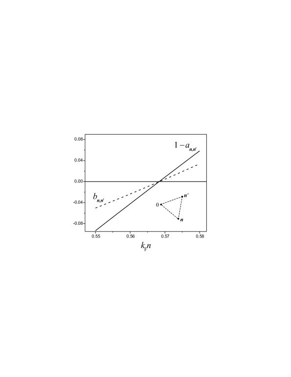
Figure 1: An example of simultaneous solution of the two conditions, $a_{\mathbf{n},\mathbf{n}^{\prime}}=1$ and $b_{\mathbf{n},\mathbf{n}^{\prime}}=0$, necessary for impurity triples to contribute into the in-gap DOS of a planar SC system. Inset: the chosen geometry of equilateral triangle $0,\mathbf{n},\mathbf{n}^{\prime}$.

But for the next, triple term of GE, which contains the inverse of the matrix (see, e.g., Ref. ip ):

$$1-2\widehat{A}_{0,\mathbf{n}}^{0}\widehat{A}_{0,\mathbf{n}^{\prime}}^{0}\widehat{A}_{\mathbf{n},\mathbf{n}^{\prime}}^{0}-\left(\widehat{A}_{0,\mathbf{n}}^{0}\right)^{2}-\left(\widehat{A}_{0,\mathbf{n}^{\prime}}^{0}\right)^{2}-\left(\widehat{A}_{\mathbf{n},\mathbf{n}^{\prime}}^{0}\right)^{2}=$$

$$=1-\widehat{M}\left(a_{\mathbf{n},\mathbf{n}^{\prime}},b_{\mathbf{n},\mathbf{n}^{\prime}}\right),$$ (27)

the conditions by Eq. 25 turn already realizable. They are explicitly formulated as follows:

$$a_{\mathbf{n},\mathbf{n}^{\prime}}=2\mathcal{F}_{0,\mathbf{n}}\mathcal{F}_{0,\mathbf{n}^{\prime}}\mathcal{F}_{\mathbf{n},\mathbf{n}^{\prime}}\cos\left(\varphi_{\mathbf{n}}+\varphi_{\mathbf{n}^{\prime}}+\varphi_{\mathbf{n}-\mathbf{n}^{\prime}}\right)+$$

$$+\mathcal{F}_{0,\mathbf{n}}^{2}\cos 2\varphi_{\mathbf{n}}+\mathcal{F}_{0,\mathbf{n}^{\prime}}^{2}\cos 2\varphi_{\mathbf{n}^{\prime}}+$$

$$+\mathcal{F}_{\mathbf{n},\mathbf{n}^{\prime}}^{2}\cos 2\varphi_{\mathbf{n}-\mathbf{n}^{\prime}}=1,$$ (28)

and

$$b_{\mathbf{n},\mathbf{n}^{\prime}}=2\mathcal{F}_{0,\mathbf{n}}\mathcal{F}_{0,\mathbf{n}^{\prime}}\mathcal{F}_{\mathbf{n},\mathbf{n}^{\prime}}\sin\left(\varphi_{\mathbf{n}}+\varphi_{\mathbf{n}^{\prime}}+\varphi_{\mathbf{n}-\mathbf{n}^{\prime}}\right)+$$

$$+\mathcal{F}_{0,\mathbf{n}}^{2}\sin 2\varphi_{\mathbf{n}}+\mathcal{F}_{0,\mathbf{n}^{\prime}}^{2}\sin 2\varphi_{\mathbf{n}^{\prime}}+$$

$$+\mathcal{F}_{\mathbf{n},\mathbf{n}^{\prime}}^{2}\sin 2\varphi_{\mathbf{n}-\mathbf{n}^{\prime}}=0.$$ (29)

The easiest localization of quasiparticles of course is expected at the very edge of the gap: $\varepsilon\rightarrow\Delta$, where ${\textrm{e}}^{-|\mathbf{n}|/r_{\varepsilon}}\rightarrow 1$. Then, e.g., for $v\approx 1.728$ it is achieved with $|\mathbf{n}|=|\mathbf{n}^{\prime}|=|\mathbf{n}-\mathbf{n}^{\prime}|\approx 0.566k_{\mathrm{F}}^{-1}$, as shown in Fig. 1, and it can be also reached for close values of $v$ by small adjustments of the distances.

Once such a pole exists, we can introduce in the configuration space of triangles $0,\mathbf{n},\mathbf{n}^{\prime}$, in the vicinity of this pole, the effective variables:

$$r=\sqrt{\left(1-a_{\mathbf{n},\mathbf{n}^{\prime}}\right)^{2}+b_{\mathbf{n},\mathbf{n}^{\prime}}^{2}},\quad\varphi=\arctan\frac{b_{\mathbf{n},\mathbf{n}^{\prime}}}{1-a_{\mathbf{n},\mathbf{n}^{\prime}}},$$

and a certain $z$, independent of $r,\,\varphi$, arriving at the general form for $\rho_{3}\left(\varepsilon\right)$ as an integral

$$\rho_{3}\left(\varepsilon\right)=c^{3}{\textrm{Im}}\int\frac{F\left(r,\varphi,z\right)}{r}dr\>d\varphi\>dz=$$

$$=2\pi c^{3}\int F\left(0,\varphi,z\right)d\varphi\>dz.$$

Here the function

$$F\left(r,\varphi,z\right)=2(a_{z,\varphi}\cos\varphi+b_{z,\varphi}\sin\varphi)J(r,\varphi,z)$$

contains the $\widehat{M}$-algebra coefficients $a_{z,\varphi},\>b_{z,\varphi}$ related to a certain matrix numerator in the triple GE term (see its explicit form in Ref. ip ) and the Jacobian $J(r,\varphi,z)$ of transition from $\mathbf{n},\mathbf{n}^{\prime}$ to the effective variables. Apart from technical details of calculation, this contribution $\sim c^{3}\rho_{{\textrm{F}}}$ can be routinely obtained.

It should be noted however that the above approach uses the asymptotical form, Eq. 18, of interaction functions, so it is only justified if the resulting poles, like that in Fig. 1, are related to long distances $n\gg a$. This is easier achieved if $ak_{{\textrm{F}}}\ll 1$ for the host crystal, as is the case for HTSC systems, but hardly for common s-wave superconductors. In the latter case, the finite in-gap DOS should result more probably from high enough terms of GE.

Another important aspect is the analysis of convergency of matrix GE’s, Eqs. 12, 14, permitting to distinguish between band-like and localized spectrum areas in the non-uniform SC system. This can be realized, using the above estimates for the non-renormalized functions $\widehat{A}_{0,\mathbf{n}}^{0}$ and $\widehat{T}^{0}$ as approximations for the renormalized ones $\widehat{A}_{0,\mathbf{n}}$ and $\widehat{T}$ in the region of band-like states $\varepsilon>\Delta$.

A similar algebraic techniques can be also developed for the d-wave SC systems, related in that case to the impurity resonance states. In this situation, the higher DOS corrections $\rho_{2,\ldots}$ to non-zero $\rho_{0}+\rho_{1}$ within the gap can be not so pronounced as for the zero-background case of s-wave system. Nevertheless the important criteria for GE convergence can be obtained, permitting a more consistent validation of T-matrix approximation and demarcation between band-like and localized states, compared to the recently suggested check based on the phenomenological Ioffe-Regel criterion lp .

References

• (1) M.A. Ivanov, Sov. Phys. Sol. State, 12, 1508 (1971).
• (2) Yu.G. Pogorelov, Solid State Commun. 95, 245 (1995).
• (3) J.E. Mayer, M. Goeppert-Mayer, Statistical Mechanics, Wiley, N.Y. (1977).
• (4) M.A. Ivanov, V.M. Loktev, Yu.G. Pogorelov, Phys. Rep., 153, 209 (1987).
• (5) P.W. Anderson, J. Phys. Chem. Solids, 3, 11 (1959).
• (6) E.N. Economou, Green’s Functions in Quantum Physics, Springer, Berlin (1983).
• (7) L.P. Gor’kov, Sov. Phys. JETP, 7, 505 (1958).
• (8) G. Baym, Phys. Rev. 127, 1391 (1962).
• (9) M.A. Ivanov, Yu.G. Pogorelov, Sov. Phys. JETP, 45, 1155 (1977).
• (10) V.M. Loktev, Yu.G. Pogorelov, Phys. Lett. A (to be published).