Heat Transport through Rough Channels

Abstract

We investigate the two-dimensional transport of heat through viscous flow between two parallel rough interfaces with a given fractal geometry. The flow and heat transport equations are solved through direct numerical simulations, and for different conduction-convection conditions. Compared with the behavior of a channel with smooth interfaces, the results for the rough channel at low and moderate values of the Péclet number indicate that the effect of roughness is almost negligible on the efficiency of the heat transport system. This is explained here in terms of the Makarov’s theorem, using the notion of active zone in Laplacian transport. At sufficiently high Péclet numbers, where convection becomes the dominant mechanism of heat transport, the role of the interface roughness is to generally increase both the heat flux across the wall as well as the active length of heat exchange, when compared with the smooth channel. Finally, we show that this last behavior is closely related with the presence of recirculation zones in the reentrant regions of the fractal geometry.

I Introduction

The study of transport phenomena in irregular media is fully recognized nowadays as an important research subject with many technological and industrial applications. In particular, the role of the morphology of an active interface on the efficiency of heat and mass transport devices has also been a theme of great interest for the scientific community. For example, the development of a modern approach for the project of heat exchangers must necessarily take the detailed description of the surface geometry as a possibility for the proper design of these devices. It is well-known in this field that the inclusion of extended surfaces or fins to the surface of the heat exchanger can substantially increase the rate of heat transfer in the system and, therefore, the efficiency of the equipment Arpaci66 ; Incropera90 .

For all practical purposes, the restrictions imposed to the geometrical features of an exchange interface should be the result of an intimate balance between its complexity and cost from one side, and the performance of the equipment from the other. In any case, an important issue in the design of heat exchangers is certainly the extent to which the heat transfer capacity of the system is dictated by the available surface area. For instance, under diffusion-limited conditions, the access of heat to an irregular surface can be highly nonuniform due to screening effects. In this situation, the regions corresponding to fins or extended protrusions will display a higher activity as opposed to the deep parts of fjords which are more difficult to access. As a result, under strong diffusive constraints, the efficiency of the surface for heat exchange can be substantially different from the one expected, considering its total area, the intrinsic conductive properties of the material, and the transport properties of the heating (or cooling) fluid.

An analogous problem can be found in the context of electrochemistry. The nonuniform activity during the linear transport through irregular interfaces of electrodes has been explained in terms of a screening effect which is entirely similar to the one observed in heat transfer. The extensive research developed on this subject in recent years Sapoval94 ; Pfeifer95 ; Sapoval96 has been mainly devoted to the introduction, calculation and application of the concept of active zone in the Laplacian transport to and across irregular interfaces. For example, through the coarse-graining method proposed in Sapoval94 it is possible to compute the flux through electrode surfaces from their geometry alone, without solving the general Laplace problem. In a subsequent study Sapoval01 , it has been shown that this technique provides consistent predictions for the activity of irregular catalyst surfaces. More recently, the activity of irregular absorbing interfaces operating under diffusion-limited conditions has been investigated through nonequilibrium molecular dynamics Andrade03 . The simulation results indicate that the extent of the interface that is significantly active is rather sensitive to the governing mechanism of transport. Precisely, the length of the active zone decreases continuously with density from the Knudsen to the molecular diffusion regime.

The study of laminar-forced-convective heat transfer through tubes or between parallel plates with smooth walls is well known in the literature as the Graetz problem Graetz . Graetz solved the problem analytically with the assumptions of steady, irrotational and incompressible flow, constant fluid properties, fully developed velocity profiles, and in the absence of energy dissipation effects. Much effort has been dedicated in the past years to improve the accuracy of the Graetz solution and generalize the Graetz problem to include other types of boundary conditions Randall97 ; Dennis56 ; Coelho01 ; Telles02 ; Sellars56 ; Brown60 ; Mikhailov97 . The development and solution of more realistic models for heat transport in internal flow configurations and under forced convection conditions has also been a research theme of great scientific interest Johnston94 ; Papoutsakis81 ; Lahjomri03 . Few studies, however, have been dedicated to the investigation of an important extension of the Graetz problem, namely, the case in which the flow and heat transfer processes are confined to walls of irregular geometry.

In the present work we apply the concept of active zone to investigate the steady-state transport of heat in a fluid flowing through a two-dimensional channel whose walls are irregular interfaces. We investigate through direct computational simulations the effect of the interface geometry on the heat exchange efficiency of the system for different diffusive(conductive)-convective conditions. Compared to the behavior of a smooth channel under conditions where the convective mechanism of transport is relevant, our results show that the activity of the interface can be significantly underestimated if geometrical details are not adequately considered.

This paper is organized as follows. In Section 2, we introduce the general description of the physical system and study the flow through the irregular geometry. The transport of heat through the flowing fluid in the rough channel is then numerically treated in Section 3. Finally, general conclusions and perspectives are drawn in Section 4.

II Viscous flow between rough interfaces

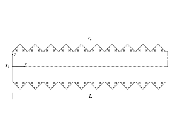
Figure 1: Schematic diagram of the rough channel under study. The walls are a sequence of irregular interfaces with the geometry of square Koch trees. The fluid flows steadily from left to right at $Re\approx 1$. A constant temperature $T_{0}$ is maintained at the inlet, while the temperature on both walls is $T_{w}$. We study the steady-state transport of heat for the case in which $T_{0}>T_{w}$, i.e., the heat goes from the bulk of the fluid to the walls of the channel.

As shown in Fig. 1, our physical system is a two-dimensional channel of length $L$ whose delimiting walls are identical interfaces with arbitrary geometry separated by a distance $2h$. By definition, the two interfaces are made by the connection of several wall subsets. In the particular roughness model adopted here, we consider that these subsets are identical pre-fractal curves with the geometry of a square Koch tree Evertsz92 .

The mathematical description for the detailed fluid mechanics in the channel is based on the assumptions that we have a continuum, Newtonian and incompressible fluid flowing under steady state conditions. Thus, the Navier-Stokes and continuity equations reduce to

$$\rho\left[u{\partial u\over\partial x}+v{\partial u\over\partial y}\right] = -{\partial p\over\partial x}+\mu\left[{\partial^{2}u\over\partial x^{2}}+{\partial^{2}u\over\partial y^{2}}\right]~{},$$ (1)

$$\rho\left[u{\partial v\over\partial x}+v{\partial v\over\partial y}\right] = -{\partial p\over\partial y}+\mu\left[{\partial^{2}v\over\partial x^{2}}+{\partial^{2}v\over\partial y^{2}}\right]~{},$$ (2)

$${\partial u\over\partial x}+{\partial v\over\partial y} = 0~{}.$$ (3)

Here the independent variables $x$ and $y$ denote the position in the channel, $u$ and $v$ are the components of the velocity vector in the $x$ and $y$ directions, respectively, and $p$ is the local pressure in the system. The relevant physical properties of the flowing fluid are the density $\rho$ and the viscosity $\mu$. In our simulations, we consider non-slip boundary conditions at the entire solid-fluid interface. In addition, the changes in velocity rates are assumed to be zero at the exit $x=L$ (gradientless boundary conditions), whereas a parabolic velocity profile is imposed at the inlet of the channel,

$$u(0,y)=\frac{3}{2}V[1-{(\frac{y}{h})}^{2}]~{}.$$ (4)

The Reynolds number is defined here as $Re\equiv{\rho Vh/\mu}$, where $V$ is the average velocity at the inlet. For simplicity, we restrict our study to the case where the Reynolds number is sufficiently low ($Re\approx 1$) to ensure a laminar viscous regime for fluid flow. Finally, we also assume that the fluid density and viscosity are constant properties of the flow throughout the channel. As a consequence, the flow field is decoupled from temperature and can be independently calculated.

The numerical solution of Eqs. (1)-(3) for the velocity and pressure fields in the rough channel is obtained through discretization by means of the control volume finite-difference technique Patankar80 . For the complex geometry involved, we solve this problem using a structured mesh based on quadrangular grid elements. For example, in the case of the channel with walls subsets that are 3-generation Koch curves, a total of 79,200 cells generates satisfactory results when compared with numerical meshes of small resolution. The integral form of the governing equations is then considered at each cell of the numerical grid to produce a set of algebraic equations which are pseudo-linearized and solved using the SIMPLE algorithm Patankar80 . The criteria for convergence used in the simulations is defined in terms of residuals, i.e., a measure of the degree to which the conservation equations are satisfied throughout the flow field. In all simulations we performed, convergence is considered to be achieved only when each of the residuals fall below $10^{-6}$.

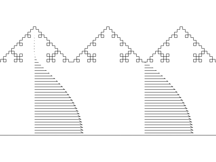
Figure 2: Longitudinal velocity profiles at two distinct cross-sections of the rough channel. Although small when compared to the mainstream flow, the velocities inside the reentrant zones of the pre-fractal geometry are not equal to zero, as can be observed in the profile on the left. At the cross-section on the right, the velocity profile is typically parabolic.

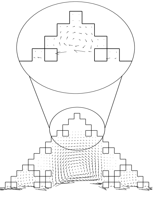
Figure 3: Vortices in the reentrant zones of the pre-fractal roughness. A close-up view of a smaller roughness detail reveals the sequence of eddies with intensities that fall off in geometric progression.

In Fig. 2 we show the velocity profiles corresponding to two different sections of the rough channel along its longitudinal direction. Although very small when compared to the velocities at the center, the velocities of the fluid cells constituting the reentrant zones are still finite. Indeed, as depicted in Fig. 3, a close-up of these roughness details shows fluid layers in the form of consecutive eddies whose intensities fall off in geometric progression Moffat64 ; Leneweit99 . Although much less intense than the mainstream flow, these recirculating structures are located deeper in the system, and therefore experience closer the landscape of the solid-fluid interface. More precisely, viscous momentum is transmitted laterally from the mainstream flow and across successive laminae of fluid to induce vortices inside the fractal cavity. These vortices will then generate other vortices of smaller sizes and intensities. In the next section, we show how this flow structure affects the overall transport of heat as well as the distribution of fluxes among the active wall elements in the rough channel.

III Heat transport

Once the velocity and pressure fields are obtained for the flow in the rough channel, we proceed with the mathematical modeling and numerical computation of the temperature scalar field. As already mentioned, we assume that the flow is independent of the temperature. In practice, we simply “freeze” the velocity field solution previously calculated and use it to compute the steady-state temperature field $T(x,y)$ solving the two-dimensional diffusion-convection equation,

$$u\frac{\partial T}{\partial x}+v\frac{\partial T}{\partial y}=\alpha\left(\frac{\partial^{2}T}{\partial x^{2}}+\frac{\partial^{2}T}{\partial y^{2}}\right)~{},$$ (5)

where $\alpha\equiv k/\rho c_{p}$ is the thermal diffusivity, $k$ is the thermal conductivity, and $c_{p}$ is the specific heat of the fluid. For boundary conditions, we consider that the inlet is subjected to a constant temperature $T_{0}$ and that the temperature $T_{w}$ is imposed on both wall interfaces. In particular, we study the case in which $T_{0}>T_{w}$, i.e., the heat is transported from the bulk of the fluid to the walls of the rough channel. The relative influence of the conductive (diffusive) and convective mechanisms of heat transport on the behavior of the system is quantified here in terms of the Péclet number, defined as

$$Pe\equiv Vh^{2}/\alpha L~{}.$$ (6)

Similarly to the procedure already utilized for the calculation of the flow, the temperature $T(x,y)$ is also obtained through discretization of Eq. (5) by means of finite-differences, with an upwind scheme to avoid numerical instabilities due to the presence of convection Patankar80 . Using this numerical technique, simulations have been performed for three types of channels corresponding to the first three pre-fractal generations of the square Koch tree.

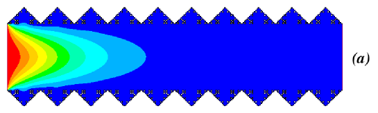
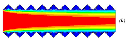
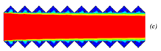
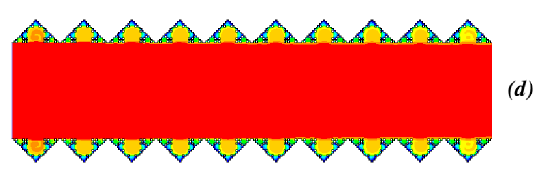
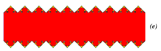
Figure 4: Contour plot of the temperature field for different values of the Péclet number: (a) $Pe=0.25$, (b) $Pe=10$, (c) $Pe=200$, (d) $Pe=10^{5}$, and (e) $Pe=10^{7}$. The temperature decreases from red (gray dark) to blue (gray light).

In Fig. 4 we show contour plots of the temperature field in a 3-generation channel for four different diffusion-convection conditions. At very low $Pe$ (Fig. 4a), conduction is the dominant mechanism with the transport of heat being practically limited to the entrance region of the channel. By increasing the value of $Pe$ (Figs. 4b-d), the contribution of convection to heat transfer through the center of the channel becomes relevant. As shown in Fig. 4c, although the inlet temperature can reach the exit at $Pe\approx 200$, the temperature at the reentrant zones of the wall remains virtually unaffected by convection. Only at very high values of $Pe$, when the vortices inside these irregularities can effectively transport heat, the high temperature front can penetrate deeper in the system (Fig. 4e).

The role of the wall roughness on the transport of heat in the channel can be quantified in terms of the normalized heat flux

$$\phi\equiv q_{w}/q_{0}~{},$$ (7)

where $q_{w}$ is the total heat flux crossing the fluid-solid interface from the bulk,

$$q_{w}=-k\displaystyle\int_{surf}~{}\frac{\partial T}{\partial n}~{}ds~{}.$$ (8)

The reference value $q_{0}$ corresponds to the heat flux crossing a smooth interface of size $L$ at temperature $T_{w}$ that is part of a system where heat is transported by conduction through a static fluid from a line at a fixed temperature $T_{0}$,

$$q_{0}=k\frac{T_{0}-T_{w}}{h}L~{}.$$ (9)

The dependence of the flux $\phi$ on the $Pe$ number is shown in Fig. 5 for the first three generations of the selected pre-fractal geometry. The behavior of a smooth channel of size $L$ and subjected to the same boundary conditions is also shown for comparison. In this simpler case, the system displays a sharp increase of the flux with $Pe$, up to a point ($Pe\approx 10$) where the following power-law regime persists for more than 5 orders of magnitude:

$$\phi\sim Pe^{1/3}~{}.$$ (10)

This behavior has been observed in previous theoretical studies Sellars56 . In the case of the power-law, it has been demonstrated that the analytical solution of the classical Graetz problem, where the mechanism of axial conduction is disregarded, converges asymptotically to this scaling behavior Sellars56 . Alternatively, as we show in the Appendix, this typical power-law regime of heat transport, known to be valid for moderate and high $Pe$ values, can be readily recovered by means of a global heat balance on the system combined with a simple scaling argument.

Remarkably, the results shown in Fig. 5 indicate that different rough channels display approximately the same behavior for low and moderate $Pe$ numbers ($Pe<200$). Moreover, their performances are also similar to the behavior of the smooth channel for the same range of $Pe$ values. Under these conditions, the conduction of heat either predominates over convection or still represents a significant contribution to the overall flux across the walls.

For Péclet values in the range $10<Pe<200$, each pre-fractal subset of the interface with the surrounding fluid can be approximately taken as a purely diffusive cell subjected to a constant temperature $T_{w}$ at the wall, and a temperature $T_{0}$ at a line in the bulk of the fluid separated by a given distance from the center of the channel. Considering steady-state conditions, the system can then be treated as a two-dimensional Laplacian transport unit subjected to Dirichlet’s boundary condition. This is a typical situation where the the theorem of Makarov holds Makarov85 . This theorem states that the information dimension of the harmonic measure on a singly connected interface in $d=2$ is exactly equal to 1, where $d$ represents dimension. Makarov’s theorem has a simple but important consequence: the screening effect due to geometrical irregularities of the interface can be accessed in terms of the ratio $S\equiv L_{p}/L$ Sapoval94 , where $L_{p}$ is the perimeter of the interface. Because the active length of the interface $L_{a}$ is of the order of the system size, $L_{a}\approx L$, then $L_{a}\approx L_{p}/S$ and the factor $S$ can be considered as the “screening factor” of the Dirichlet-Laplacian field. When applied to our physical system, the practical meaning of this exact result is that, irrespective of the surface morphology, the length of the zone within the heat exchange wall which receives most of the heat flux should be of the order of the system size $L$, instead of the perimeter $L_{p}$. This explains why in Fig. 5 the heat flux at the interface is nearly insensitive to differences in the roughness geometry for low and moderate values of $Pe$.

For $Pe>200$, the predominance of convection over conduction is extended to the reentrant zones of the pre-fractal units. This crossover value results from the fact that the magnitudes of the velocity vectors constituting the largest vortices in the rough region are approximately two orders of magnitude smaller than the main flow velocity $V$. At high $Pe$ values, heat can then be convected through these recirculating structures of the flow towards the less accessible wall elements of the interface. Under such circumstances, the theorem of Makarov is not valid anymore, and the flux $\phi$ across the wall becomes dependent on the geometrical details of the interface. As shown in Fig. 5, the higher the generation of the pre-fractal interface, larger is the heat flux at high Péclet conditions.

We now show that the previous analysis based on the overall heat flux $\phi$ is consistent with the behavior of a more detailed measure of transport. In particular, the flux heterogeneity at the interface can be quantified in terms of an active length defined as Sapoval99

$$L_{a}\equiv 1/\sum_{i=1}^{L_{p}}\phi_{i}^{2}~{}~{}~{}~{}(1\leq L_{a}\leq L_{p})~{},$$ (11)

where the sum is over the total number of interface elements $L_{p}$, $\phi_{i}\equiv q_{i}/\sum q_{j}$, and $q_{i}$ is the thermal flux at the wall element $i$. From the definition (11), $L_{a}=L_{p}$ indicates a limiting state of equal partition of normalized fluxes (${\phi_{i}}=1/L_{p}$, $\forall i$) whereas $L_{a}=1$ should correspond to the case of a fully “localized” flux distribution. The active length therefore provides an useful index to quantify the interplay between the Laplacian phenomenology and the complex geometry of the absorbing interface at the local scale. As expected, the results shown in Fig. 6 indicate that $L_{a}$ generally increases with $Pe$. It is important to note, however, that the activities of smooth and rough interfaces behave approximately in the same way for low values of $Pe$. This is also consistent with Makarov’s theorem under conditions where the conduction mechanism controls the transport of heat inside the pre-fractal roughness.

For high Péclet values, $L_{a}$ becomes strongly sensitive to the geometrical details of the interface. Again, due to the relevant contribution of convection to the transport at the smaller scales, the flux distribution among the interface units becomes more uniform. The higher the pre-fractal generation used to create the roughness geometry, higher is the available number of wall elements for heat exchange. As a consequence, a substantial increase in the active length can be observed for a fixed value of $Pe$.

IV Conclusions

The development of a coherent scientific approach to the project of heat and mass transport devices involving new concepts from mathematics and physics still represents an important research and technological challenge to chemical and mechanical engineers. In the present work, we have studied the conditions under which the roughness geometry of a channel with a flowing fluid should play a relevant role on the transport of heat. For low Péclet numbers, when the mechanism of heat conduction dominates, it is shown that the overall flux of heat across a pre-fractal interface subjected to Dirichlet boundary conditions has little sensitivity to details and irregularities of the heat absorption zone. Under similar conditions, the length of the active zone computed for a smooth channel is very close to the measure obtained for a rough system. This behavior is then interpreted in terms of a screening phenomenon that privileges the absorbing activity of the geometrically exposed sites of the interface. Moreover, such a “localization” of the heat flux can be formally explained in terms of Makarov’s theorem for Laplacian transport in two-dimensional irregular geometries.

The situation is entirely different at high Péclet numbers. In this case, our simulations reveal that both the heat flux and the active length start to depend noticeably on the morphological details of the interface. In this situation, not only the total heat flux leaving the system increases faster for higher generations of the pre-fractal interface, but the distribution of fluxes at the wall units also becomes gradually less “localized” ($L_{a}$ increases) as $Pe$ increases. This transition reflects the onset of convective effects on the heat transport in the proximity of the rough interface. A closer look at the system indicates that the significant changes observed in $L_{a}$ above the transition point are induced by the presence of recirculation zones of flow (vortices) in these regions.

As a future work, we will extend the approach introduced here to simulate the effect of different geometries on the transport efficiency of the system as well as other types of “absorption” mechanisms (e.g., finite-rate heat transfer at the walls) limited by diffusion transport. Finally, we also believe that the results presented in this study provide useful information to the understanding of other physico-chemical systems with relevance to science and technology that include heat, mass or momentum transport. The modeling strategy devised here should also be helpful as a design tool to choose a suitable interface geometry for a given heat exchange system.

V Acknowledgments

We thank Bernard Sapoval and Marcel Filoche for many helpful discussions. We acknowledge the Brazilian agencies CNPq, CAPES and FUNCAP for financial support.

VI Appendix: The smooth channel

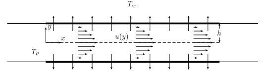
Figure 7: Schematic diagram of the smooth channel showing the fully developed parabolic profile of the flow. As in the case of the rough channel, the inlet is at temperature $T_{0}$ while the temperature on both walls is maintained at $T_{w}$. We also consider the case in which $T_{0}>T_{w}$.

Here we revisit the classical problem of heat transport through a fluid flowing in a channel whose walls are smooth interfaces. The system setup is shown in Fig. 7. As in the case of the rough channel, we consider a Newtonian and incompressible fluid with constant properties that is flowing under viscous and steady-state conditions. Assuming non-slip boundary conditions at the walls, the velocity along the channel follows the classical parabolic profile

$$u=\frac{3}{2}V(1-{\eta}^{2})~{},$$ (12)

where $\eta\equiv y/h$, $V\equiv\Delta p~{}h/(3\mu L)$, and $\Delta p$ is the pressure drop between the entrance and the exit of the channel. Under these simple flow conditions, the fluid is suddenly subjected to the temperature $T_{0}$ at the channel inlet, while a constant temperature $T_{w}$ is imposed at both walls. At steady-state, and assuming that the axial heat conduction mechanism is negligible, this corresponds to the so-called Graetz problem, where the temperature field in the channel obeys the following differential equation:

$$u(y)\frac{\partial T}{\partial x}=\alpha\frac{\partial^{2}T}{\partial y^{2}}~{},$$ (13)

with boundary conditions

$$T(0,y)=T_{0}~{}~{}~{}~{}~{}\text{and}~{}~{}~{}~{}~{}T(x,h)=T_{w}~{}.$$ (14)

An analytical solution for the linear partial differential equation (13) subjected to (14) can be obtained through separation of variables and a proper expansion in terms of the so-called Graetz functions Arpaci66 ; Sellars56 . From this solution, it is possible to show that the overall heat flux through the absorbing walls, $\phi$, follows the power law behavior, $\phi\sim Pe^{1/3}$, that is valid for moderate and high $Pe$ values.

The objective here is to show that this power-law regime of heat transport can be readily recovered by means of a global heat balance combined with a simple scaling argument. First, in the absence of sources or sinks of heat, the total heat crossing the walls should be equal to the difference

$$q_{w}=q_{in}-q_{out}~{},$$ (15)

where $q_{in}$ and $q_{out}$ are the fluxes at the entrance and at the exit sections of the channel, respectively. At sufficiently high values of the Péclet number, the convective part of the flux dominates the heat transfer process. As shown in Fig. 8, the temperature profile at the exit displays a central plateau in the range $-y^{*}\leq y\leq y^{*}$, where the temperature is equal to the entrance temperature $T_{0}$, and then decays monotonously towards the wall temperature $T_{w}$, in the region $y^{*}\leq|y|\leq h$. The value of $\eta^{*}(\equiv y^{*}/h)$ can be found from the definition of the local Péclet number

$$Pe_{\eta}\equiv\frac{\tau_{D}}{\tau_{C}}=\frac{\delta^{2}/\alpha}{L/u(\eta)}~{},$$ (16)

where $\tau_{D}\equiv\delta^{2}/\alpha$ is the characteristic conduction time, $\tau_{C}\equiv L/u$ is the local convective time, and $\delta\equiv h(1-\eta^{*})$. If we now argue that $\eta^{*}$ should correspond to the position where $Pe_{\eta}\approx 1$, we can write from Eqs. (12) and (16) that

$$\frac{3}{2}\frac{Vh^{2}}{\alpha L}(1-\eta^{*})^{2}[1-(\eta^{*})^{2}]=1~{},$$

which, from the definition (6), leads to

$$(1-\eta^{*})^{3}(1+\eta^{*})=\frac{2}{3Pe}~{}.$$

For high values of $Pe$, $\eta^{*}$ is very close to 1, such that $(1-\eta^{*})^{3}(1+\eta^{*})\approx 2(1-\eta^{*})^{3}$, resulting in

$$\eta^{*}\approx 1-\frac{1}{(3Pe)^{1/3}}~{}.$$ (17)

Going back to Eq. (15), the heat flux $q_{in}$ entering the system is given by

$$q_{in}=2\rho c_{p}T_{0}\int^{h}_{0}u(y)\,dy~{}.$$

The flux $q_{out}$ leaving the channel can be expressed as the sum

$$q_{out}=q_{1}+q_{2}~{},$$ (18)

where the first term corresponds to the heat escaping through the plateau region of temperature $T_{0}$ and size $y^{*}$

$$q_{1}=2\rho c_{p}T_{0}\int^{y^{*}}_{0}u(y)\,dy~{},$$ (19)

while the second term represents the flux through the remaining part of the channel cross-section with variable temperature

$$q_{2}=2\rho c_{p}\int^{h}_{y^{*}}u(y)T(y)\,dy~{}.$$ (20)

As a first approximation, if we assume that the temperature in this region decreases linearly with $y$,

$$T(y)=\frac{T_{0}-T_{w}}{y^{*}-h}(y-y^{*})+T_{0}~{},$$

Eq. (20) can then be written as

$$q_{2} = 2\rho c_{p}T_{0}\int^{h}_{y^{*}}u(y)\,dy$$

$$+ 2\rho c_{p}\int^{h}_{y^{*}}u(y)\frac{T_{0}-T_{w}}{y^{*}-h}(y-y^{*})\,dy~{},$$

and the total flux becomes

$$q_{w}=2\rho c_{p}\frac{T_{0}-T_{w}}{h-y^{*}}\int_{y^{*}}^{h}\frac{3}{2}V\left[1-\left(\frac{y}{h}\right)^{2}\right](y-y^{*})dy~{}.$$

Rewriting this expression in terms of the dimensionless variable $\eta$, we obtain

$$q_{w} = 3\rho c_{p}(T_{0}-T_{w})Vh\frac{1}{1-\eta^{*}}\int_{\eta^{*}}^{1}\left(1-\eta^{2}\right)(\eta-\eta^{*})d\eta$$

$$= \frac{3}{12}\rho c_{p}(T_{0}-T_{w})Vh\left[(\eta^{*})^{3}+(\eta^{*})^{2}-5\eta^{*}+3\right]~{}.$$

From this equation and the definitions (6) and (7), the normalized flux can be expressed as

$$\phi=\frac{3}{12}Pe\left[(\eta^{*})^{3}+(\eta^{*})^{2}-5\eta^{*}+3\right]~{},$$

and using the approximation (17), we finally get the scaling relation

$$\phi\approx\frac{\left(3Pe\right)^{1/3}}{3}-\frac{1}{12}~{}.$$ (21)

Figure 5: Log-log plot showing the dependence of the normalized flux across the walls, $\phi$, on the Péclet number, $Pe$. The solid line represents the behavior of a smooth channel, while the dashed, dot-dashed and dotted lines correspond to the first, second and third pre-fractal generations, respectively.

Figure 6: Logarithmic plot showing the variation of the length of the active zone, $L_{a}$, with the Péclet number, $Pe$. The solid line corresponds to the case of a smooth channel, while the dashed, dot-dashed and dotted lines represent the behavior of the first, second and third pre-fractal generations, respectively.

Figure 8: Steady-state profiles of the normalized temperature at the exit of the smooth channel for three different values of the Péclet number.

References

- (1) V. S. Arpaci, Conduction Heat Transfer (Addison-Wesley, Reading, MA, 1966).
- (2) F. P. Incropera and D. P. DeWitt, Fundamentals of Heat and Mass Transfer (John Wiley & Sons, New York, 1990).
- (3) B. Sapoval, Phys. Rev. Lett. 73, 3314 (1994).
- (4) Pfeifer and B. Sapoval, Mat. Res. Soc. Symp. Proc. 366, 271 (1995).
- (5) B. Sapoval, in Fractals and Disordered Systems, 2nd ed., edited by A. Bunde and S. Havlin, (Springer-Verlag, Berlin, 1996), p.232.
- (6) B. Sapoval, J. S. Andrade Jr., and M. Filoche, Chem. Eng. Sci. 56, 5011 (2001); J. S. Andrade Jr., M. Filoche, and B. Sapoval, B., Europhys. Lett. 55, 573 (2001).
- (7) J. S. Andrade Jr., H. F. da Silva, M. Baquil, and B. Sapoval Phys. Rev. E 68, 041608 (2003).
- (8) L. Graetz, Ann. Phys. Chem. 25, 337 (1885).
- (9) R. F. Barron, X. Wang, T. A. Ameel, and R. Warrington, Int. J. Heat Mass Tran. 40, 1817 (1997).
- (10) S. C. R. Dennis and G. Poots, Q. Appl. Math. 14, 231 (1956) .
- (11) R. M. Coelho and A. S. Telles, Int. J. Heat Mass Tran. 45, 3101 (2002).
- (12) A. S. Telles, E. M. Queiroz, and G. Elmor, Int. J. Heat Mass Tran. 44, 471 (2001).
- (13) J. R. Sellars, M. Tribus, and J. S. Klein, Transactions of the ASME 78, 441 (1956).
- (14) G. M. Brown, A.I.Ch.E. J. 6, 179 (1960).
- (15) M. D. Mikhailov and R. M. Cotta, Int. Commun. Heat Mass 24, 449 (1997).
- (16) P. R. Johnston, Math. Comput. Model. 19, 1 (1994).
- (17) E. Papoutsakis and D. Ramkrishna, Chem. Eng. Sci. 36, 1381 (1981).
- (18) J. Lahjomri, K. Zniber, A. Oubarra, and A. Alemany, Energ. Convers. Manage. 44, 11 (2003).
- (19) C. J. G. Evertsz and B. B. Mandelbrot, J. Phys. A: Math. Gen. 25 1781 (1992).
- (20) S. V. Patankar, Numerical Heat Transfer and Fluid Flow (Hemisphere, Washington DC, 1980); We use the FLUENT fluid dynamics analysis package (FLUENT Inc.) in this study.
- (21) H. K. Moffat, J. Fluid. Mech. 18, 1 (1964).
- (22) G. Leneweit and D. Auerbach, J. Fluid Mech. 387, 129 (1999).
- (23) N. G. Makarov, Proc. London Math. Soc. 51, 369 (1985); P. Jones and T. Wolff, Acta Math. 161, 131 (1988).
- (24) B. Sapoval, M. Filoche, K. Karamanos, and R. Brizzi, Eur. Phys. J. B 9, 739 (1999).