On electronic shells surrounding charged insulated metallic clusters

Abstract

We determine the wavefunctions of electrons bound to a positively charged mesoscopic metallic cluster covered by an insulating surface layer. The radius of the metal core and the thickness of the insulating surface layer are of the order of a couple of ångström. We study in particular the electromagnetic decay of externally located electrons into unoccupied internally located states which exhibits a resonance behaviour. This resonance structure has the consequence that the lifetime of the “mesoscopic atoms” may vary by up to 6 orders of magnitude depending on the values of the parameters (from sec to years).

1 Introduction

Clusters consisting of some 10² to 10⁵ atoms, which can be produced for instance in the course of the condensation of vapour, have attracted great interest during the last 20 years. These ”mesoscopic” clusters were found to exhibit classical as well as quantum mechanical features. In the special case of metallic clusters [1], the conduction electrons, which move in the average potential produced by the positively charged ions, exhibit shell effects. As a consequence, the binding energy of the cluster becomes a function of the number of free electrons (and thus also of the number of ions). In turn, this implies measurable variations of the formation probability of a cluster as a function of its mass in a thermal vapour-gas equilibrium.

Other interesting types of mesoscopic systems are the so-called ”fullerenes” which represent a crystal of atoms covering a closed, usually spherical surface [2]. A number of review articles exist on this exciting new field of physics (see for instance Ref. [3] and Ref. [4] and books mentioned at the end of Ref. [1] and Ref. [2]).

In the present paper, we consider a mesoscopic system which consists of a spherical metallic core of radius $R_{2}$ carrying $Z$ positive charges and surrounded by an insulating layer of external radius $R_{1}$ (see Fig. 1). We determine analytically the bound states of a single electron in the potential $V(r)$ which is produced by the positive surface charge density of the metallic core and the insulating dielectric surface layer. As in the case of an ordinary atom, these single electron wave functions describe also approximately the case that several electrons are bound in this potential. For $Z$ bound electrons, the system has total charge 0. Because of the obvious similarity of this system with an atom or ion, we refer to it as a ”mesoscopic atom” or ”mesoscopic ion”.

As one can surmise, there are two different types of bound electronic states: electrons localized in the metallic core inside of the insulating layer (region II, Fig. 1) and electrons localized in the vacuum outside of the insulating layer (region 0, Fig. 1). The bound states localized outside are reminiscent of the bound states of an electron in the Coulomb potential of the atomic nucleus. We are mainly interested in these externally localized electronic states (”class 1-states”) and their decay into lower-lying bound states predominantly localized within the metallic core (”class 2-states”).

The paper is organized as follows:

In Sec. 2, we formulate the single-particle Hamiltonian and determine the eigenfunctions and eigenenergies of bound electrons. In doing so, we take into account the polarization of the insulating surface layer which is produced by the uniform positive charge distribution on the surface $S_{2}$ of the metal, but we neglect the additional polarization effects produced by the externally localized electrons.

In Sec. 3 we determine these additional polarization effects within the classical Maxwellian electrodynamics. They lead to an additional potential acting on the electrons which is of importance close to the surface $S_{1}$ of the insulator. So far, we have not yet studied the effect of this additional potential on the externally localized electrons.

The Sec. 4 is dedicated to a presentation of the results. In Subsec. 4.1, we describe the procedure which we used in order to obtain the eigenvalues and eigenfunctions and we present typical examples of spectra and wavefunctions. In Subsec. 4.2, we discuss the electromagnetic decay of a predominantly externally localized bound electron into a lower-lying internally localized state. We show that the transition rate and the corresponding life-time may vary by several orders of magnitude depending on the parameters of the system.

In general, the transition is hindered by the small overlap between externally and internally localized states (”class 1-states” and ”class 2-states”) if the insulating surface layer is sufficiently thick. In particular, we discuss the special role in this decay of ”class 3-states” which exhibit non-negligible amplitudes both in the external region 0 and the internal region II.

Finally, in Sec. 5, we summarize the results and discuss some related open questions.

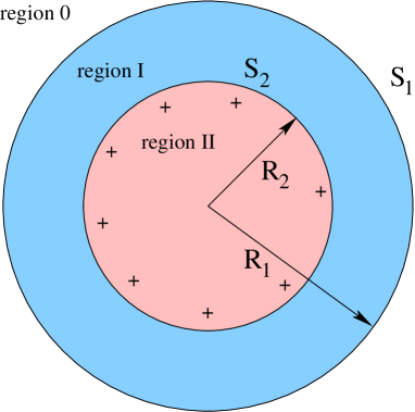
Figure 1: Schematic view of the charged metallic cluster (radius $R_{2}$, surface $S_{2}$) covered by an insulating layer (outer radius $R_{1}$, surface $S_{1}$). States of bound electrons predominantly localized in the surrounding vacuum ($R>R_{1}$, region 0) are called ”class 1-states” in distinction from states localized in the metallic core (”class 2-states”).

2 Theory

In the single-particle Hamiltonian for an electron bound to a positively charged and insulated metallic core ($M$ = mass of the electron)

$$\widehat{H}=\widehat{T}+\widehat{V}=-{\hbar^{2}\over 2M}\Delta+V(r)\,\,,$$ (1)

the potential $V(r)$ contains the interaction of the electron with the positive surplus charge $Ze_{0}$ ($e_{0}$ = elementary charge) and with the ionic background (”jellium”) of the metal. Furthermore, it contains the effects of the insulating surface layer. The radius $R_{2}$ of the metal and the thickness ($R_{1}-R_{2}$) of the surface layer are assumed to be of the order of 5 to 20 Å(1 Å= 10^-10 m) and the number $Z$ of positive charges of the metal is considered to be 1 to 5. For these dimensions of the system we may expect that, on the one hand, the dynamics of the electron is fully quantum-mechanical and, on the other hand, we may use macroscopic concepts in formulating the potential $V(r)$, at least as a first approximation. So we assume that the positive surplus charge is uniformly distributed over the surface $S_{2}$ of the metal

$$\rho_{2}(r)=\rho_{S_{2}}\cdot\delta(r-R_{2})={Ze_{0}\over 4\pi R^{2}_{2}}\delta(r-R_{2})\,.$$ (2)

The Coulomb potential produced by this simple charge distribution acting upon an electron (charge $-e_{0}$) is given by

$$-e_{0}\int d^{3}r^{\prime}{\rho_{2}(r^{\prime})\over|\vec{r}-\vec{r}^{\prime}|}=-{Ze^{2}_{0}\over R_{2}}\,\theta_{0}(R_{2}-r)-{Ze^{2}_{0}\over r}\theta_{0}(r-R_{2})\,\,,$$ (3)

where $\theta_{0}(x)$ is the Heaviside function

$$\theta_{0}(x)=\left\{\begin{array}[]{lll}1&{\rm for}&x>0\\ 0&{\rm for}&x<0\end{array}\right.\,\,.$$

Inside of the metal, the conduction electrons feel not only the constant potential produced by the positive surface charge but also the attractive interaction with the ionic background which we represent by a constant negative potential $-V^{0}_{\rm II}$ $(V^{0}_{\rm II}>0$).

On the other hand, the average energy gap above the Fermi level in the insulator may act upon the electron like a repulsive barrier of a height $B_{0}>0$.

Last not least, there are polarization effects produced by the positive surplus charge and also by the charge distribution $\rho_{e}(\vec{r})$ of the externally (i.e. predominantly in region 0) localized electrons. The polarization effects are investigated in Sec. 3 on the basis of Maxwell’s equations for the electric field $\vec{E}$ and for the displacement field $\vec{D}$ in the presence of homogeneous dielectric media. In the case that we only take into account the polarization effects produced by the positive surplus charge (2), the following modifications of the Coulomb potential (3) are to be considered: Within region I, i.e. within the insulating layer, the Coulomb potential $-Ze^{2}_{0}/r$ is to be replaced by

$$-{Ze^{2}_{0}\over r}\rightarrow-{Ze^{2}_{0}\over r\cdot\varepsilon_{\rm I}}-{Ze^{2}_{0}\cdot(\varepsilon_{\rm I}-1)\over R_{1}\cdot\varepsilon_{\rm I}}$$

and within region II, i.e. within the metallic core, the constant potential $-{Ze^{2}_{0}/R_{2}}$ is to be supplanted by

$$-{Ze^{2}_{0}\over R_{2}}\,\rightarrow\,-{Ze^{2}_{0}\over R_{2}\varepsilon_{\rm I}}-{Ze^{2}_{0}\cdot(\varepsilon_{\rm I}-1)\over R_{1}\varepsilon_{\rm I}}=-{Ze^{2}_{0}\over R_{2}}+Ze^{2}_{0}\left({1\over R_{2}}-{1\over R_{1}}\right)\left({\varepsilon_{\rm I}-1\over\varepsilon_{\rm I}}\right)\,.$$

Within region 0, i.e. in the vacuum surrounding the insulating layer, the value $-{Ze^{2}_{0}/r}$ of the Coulomb potential (3) is unchanged.

One should note that the potential in region I assumes the value $-{Ze^{2}_{0}/R_{1}}$ at the outer surface $r=R_{1}$ of the insulating layer.

Let us denote the sum of the constant parts of the potentials in region I and II by

$$B:=B_{0}-{Ze^{2}_{0}\over\varepsilon_{\rm I}R_{1}}(\varepsilon_{\rm I}-1)$$ (4)

and

$$V_{\rm II}:=V^{0}_{\rm II}-Ze^{2}_{0}\left({1\over R_{2}}-{1\over R_{1}}\right)\left({\varepsilon_{\rm I}-1\over\varepsilon_{\rm I}}\right)\,.$$ (5)

If $Z$ is equal to 1 or 2 and the dielectric constant $\varepsilon_{\rm I}$ exceeds 1 only slightly, and if the radii are in the range of values treated in Sec. 4, the 2^nd terms on the right-hand sides of Eqs. (4) and (5) are much smaller than the 1^st terms. So far, it is only these cases which we treated numerically.

Altogether, the potential $V(r)$ felt by the electron has the form

$$V(r)=-\left[V_{\rm II}+{Ze^{2}_{0}\over R_{2}}\right]\theta_{0}(R_{2}-r)+\left[B-{Ze^{2}_{0}\over\varepsilon_{\rm I}r}\right]\theta_{0}(R_{1}-r)\theta_{0}(r-R_{2})-{Ze^{2}_{0}\over r}\theta_{0}(r-R_{1})\,\,.$$ (6)

The constants $V_{\rm II}$, $\varepsilon_{\rm I}$ and $B_{0}$ are empirical parameters. The potential $V(r)$ is shown in Fig. 2 for a specific choice of the parameters.

Figure 2: Semi-quantitative picture of the potential $V(r)$ for the following choice of parameters: $R_{2}=20$ Å; $R_{1}=30$ Å; $Z=1$; $W_{0}=3.3$ eV; $V_{\rm II}=6.3$ eV; $B=3$ eV; $\varepsilon_{\rm I}=3$ ; $Ze^{2}_{0}/(\varepsilon_{\rm I}\cdot R_{2})=0.24~{}{\rm eV};Ze^{2}_{0}/(\varepsilon_{\rm I}\cdot R_{1})=0.16~{}{\rm eV};Ze^{2}_{0}/R_{1}=0.48~{}{\rm eV}\,.$

The eigenfunctions $\psi(r,\vartheta,\varphi)$ of the Schrödinger equation

$$-{\hbar^{2}\over 2M}\Delta\psi+V(r)\psi=E\psi$$ (7)

separate

$$\psi(r,\vartheta,\varphi)=R(r)Y_{lm}(\vartheta,\varphi)={u(r)\over r}Y_{lm}(\vartheta,\varphi)$$ (8)

and the radial functions $R(r)$ and $u(r)$ have to satisfy the differential equations

$$-{\hbar^{2}\over 2M}\left({d^{2}\over dr^{2}}+{2\over r}{d\over dr}-{l(l+1)\over r^{2}}\right)R+V(r)R=ER\,\,,$$ (9)

$$-{\hbar^{2}\over 2M}\left({d^{2}\over dr^{2}}-{l(l+1)\over r^{2}}\right)u+V(r)u=Eu\,\,,$$ (10)

respectively.

For $r<R_{2}$ (region II), the potential $V(r)$ is constant and thus the Eq. (9) represents the differential equation for ”spherical Bessel functions”. Of the 2 linearly independent solutions, only the regular one, $j_{l}$, qualifies as a physical solution. Up to a normalization factor which will be determined later on, the radial function $R(r)$ in region II is simply given by

$$R_{\rm II}(r)=j_{l}(\kappa_{\rm II}r)\,\,,$$ (11)

where $\kappa_{\rm II}$ is defined by

$$\kappa_{\rm II}=\sqrt{{2M\over\hbar^{2}}\left({Ze^{2}_{0}\over R_{2}}+V_{\rm II}-|E|\right)}$$ (12)

and $j_{l}(x)$ is the spherical Bessel function of the 1^st kind (see Chapt. 9 of Ref. [5]). As bound states have an energy between the well depth $-\left(V_{\rm II}+Ze^{2}_{0}/R_{2}\right)$ and 0, the parameter $\kappa_{\rm II}$ is assured to be real.

For $R_{2}<r<R_{1}$ (region I) let us postpone the treatment of the general case and first turn to the simpler situation when the $r$-dependent term $Ze^{2}_{0}/(\varepsilon_{\rm I}r)$ is negligible in comparison to the constant $B$ in the entire region I. This is so, if the inequality

$${Ze^{2}_{0}\over\varepsilon_{\rm I}R_{2}}<<B$$ (13)

holds. For the case shown in Fig. 2, the condition is fulfilled. Generally speaking, the barrier heights $B_{0}$ range from 2 to 5 eV, and the dielectric constant $\varepsilon_{\rm I}$ may have values between slightly more than 1 up to more than 100 (Examples: $\varepsilon_{\rm I}$ (caoutchouc) = 4; $\varepsilon_{\rm I}$ (Ti0₂-crystal) = 115).

Let us now investigate the case that the potential (6) can be approximated by

$$V(r)\approx-\left[V_{\rm II}+{Ze^{2}_{0}\over R_{2}}\right]\theta_{0}(R_{2}-r)+B\theta_{0}(R_{1}-r)\theta_{0}(r-R_{2})-{Ze^{2}_{0}\over r}\theta_{0}(r-R_{1})\,\,.$$ (14)

The radial Schrödinger equation (9) in region I then assumes again the form of Bessel’s differential equation. But as the energy $E$ is lower than the barrier height $B$, the solution in region I is given by a linear combination of two independent ”modified spherical Bessel functions” (see Chapt. 10.2 of Ref. [5]).

We choose the pair $\left\{(-i)^{l}j_{l}(iy),-{\pi\over 2}i^{l}h^{(1)}_{l}(iy)\right\}$, where $j_{l}(iy)$ and $h^{(1)}_{l}(iy)$ are the spherical Bessel-function and spherical Hankel-function of the 1^st kind, resp., with imaginary arguments. The dimensionless real variable $y$ is related to the radial coordinate $r$ by

$$y=\kappa_{\rm I}r\,\,,$$ (15)

$$\kappa_{\rm I}=\sqrt{{2M\over\hbar^{2}}(B+|E|)}\,\,.$$ (16)

The two factors $(-i)^{l}$ and $-{\pi\over 2}i^{l}$ are chosen so that the pair of solutions are simply related to the modified Bessel function of integer order $I_{l+{1\over 2}}(y)$ and $K_{l+{1\over 2}}(y)$ for which a number of rapidly converging series expansions exist (see Ref. [5], Chapt. 10.2)

$$\{(-i)^{l}j_{l}(iy),-{\pi\over 2}i^{l}h^{(1)}_{l}(iy)\}=\left\{\sqrt{{\pi\over 2y}}I_{l+{1\over 2}}(y),\sqrt{{\pi\over 2y}}K_{l+{1\over 2}}(y)\right\}\,\,.$$ (17)

The radial function $R(r)$ in region I thus has the general form

$$R_{\rm I}(r)=A_{\rm I}\sqrt{{\pi\over 2\kappa_{\rm I}r}}I_{l+{1\over 2}}(\kappa_{\rm I}r)+B_{\rm I}\sqrt{{\pi\over 2\kappa_{\rm I}r}}K_{l+{1\over 2}}(\kappa_{\rm I}r)\,\,.$$ (18)

For $r>R_{1}$ (region 0), it is more convenient to deal with the differential Eq. (10) for $u(r)$ which has the form

$$-{\hbar^{2}\over 2M}u^{\prime\prime}(r)+{\hbar^{2}l(l+1)\over 2Mr^{2}}u-{Ze^{2}_{0}\over r}u=Eu\,\,.$$ (19)

We have to find a normalizable solution of (19). It turns out that the only normalizable solution of (19) has the form

$$u(r)=C_{0}z^{l+1}_{0}U(a_{0},b_{0},z_{0})e^{-{z_{0}\over 2}}\,\,,$$ (20)

where the dimensionless variable $z_{0}$ is related to $r$ by

$$z_{0}=2\lambda r$$ (21)

with

$$\lambda=\sqrt{{2M|E|\over\hbar^{2}}}$$ (22)

and where $w=U(a_{0},b_{0},z_{0})$ is a particular solution Kummer’s differential equation

$$z_{0}{d^{2}w\over dz^{2}_{0}}+(b_{0}-z_{0}){dw\over dz_{0}}-a_{0}w=0\,\,.$$ (23)

The parameters $a_{0}$ and $b_{0}$ in (23) are related to the parameters in Eq. (19) by

$$a_{0}={2(l+1)-d_{0}\over 2}$$ (24)

$$b_{0}=2(l+1)$$ (25)

$$d_{0}={Ze^{2}_{0}\over\hbar}\sqrt{{2M\over|E|}}$$ (26)

and the solution $U(a_{0},b_{0},z_{0})$ of (23) is defined as follows:
We write $b_{0}$ in the form

$$b_{0}=1+n\,\,,$$ (27)

which implies

$$n=2l+1\,\,.$$ (28)

Then the function $U(a_{0},1+n,z_{0})$, where $n=1,\ldots$ reads (see Ref. [5], Eq. (13.1.6) or Ref. [6], Eq. (13) of Chapt. 6.7.1)

$$U(a_{0},n+1,z_{0}) = {(-1)^{n-1}\over n!\Gamma(a_{0}-n)}\cdot\left\{M(a_{0},n+1,z_{0})\ln z_{0}+\right.$$ (29)

$$+ \left.\sum^{\infty}_{\nu=0}{(a_{0})_{\nu}z^{\nu}_{0}\over(n+1)_{\nu}\nu!}[\psi(a_{0}+\nu)-\psi(1+\nu)-\psi(1+n+\nu)]\right\}$$

$$+ {(n-1)!\over\Gamma(a_{0})}\sum^{n-1}_{\nu=0}{(a_{0}-n)_{\nu}\over(1-n)_{\nu}}\cdot{z^{\nu-n}_{0}\over\nu!}$$

In (29), the function $\psi(x)$ is the logarithmic derivative of the $\Gamma$-function

$$\psi(x):={d\Gamma(x)\over dx}/\Gamma(x)={d\ln\Gamma(x)\over dx}$$ (30)

and $(c)_{\nu}$ is Pochhammer’s symbol

$$(c)_{\nu}:=c(c+1)\ldots(c+\nu-1)={\Gamma(c+\nu)\over\Gamma(c)}\,\,.$$ (31)

Furthermore, $M(a_{0},b_{0},z_{0})$ is the confluent hypergeometric function

$$M(a_{0},b_{0},z_{0})=\sum^{\infty}_{\nu=0}{\Gamma(a_{0}+\nu)\Gamma(b_{0})\over\Gamma(a_{0})\Gamma(b_{0}+\nu)}\cdot{z^{\nu}_{0}\over\nu!}\,\,.$$ (32)

We note in passing that the complicated form of the solution (29) is due to the fact that the parameter $b_{0}$ in $U(a_{0},b_{0},z_{0})$ is an integer. For non-integer $b_{0}$, the function $U(a_{0},b_{0},z_{0})$ depends in a simple way on two confluent hypergeometric functions (see Ref. [5], Eq. (13.1.3)). This form of $U(a_{0},b_{0},z_{0})$ becomes singular if $b_{0}$ tends to an integer value. The limiting process which leads to the form (29) is discussed in Ref. [6].

For any value of $b_{0}$, the asymptotic behaviour of $U$ for $\Re(z_{0})\rightarrow\infty$ is given by

$$U(a_{0},b_{0},z_{0})\rightarrow{1\over z^{a_{0}}_{0}}\left[1+0\left({1\over|z_{0}|}\right)\right]$$ (33)

(see Ref. [5], Eq. (13.1.8)). From (33) and (20) it is clear that $u(r)$ is a normalizable function irrespectively of the value of the energy $E$. However, it turns out that the continuity conditions can only be met for certain discrete values of $E$. The radial function $R_{0}(r)$ in region 0 is thus defined by

$$R_{0}(r)={u(r)\over 2\lambda r}=C_{0}(2\lambda r)^{l}U(a_{0},2l+2,2\lambda r)e^{-\lambda r}\,\,.$$ (34)

Before we proceed to the explicit formulation of the continuity conditions, we return to the form of the solution in region I in the general case that the $r$–dependent term $Ze^{2}_{0}/(\varepsilon_{\rm I}r)$ is not neglected. Then the differential equation for $u(r)$ in region I has the form

$$-{\hbar^{2}\over 2M}\left({d^{2}\over dr^{2}}-{l(l+1)\over r^{2}}\right)u+\left(B-{Ze^{2}_{0}\over\varepsilon_{\rm I}r}\right)u=Eu\,\,.$$ (35)

Eq. (35) resembles Eq. (19). In fact, with the replacements

$$Z\rightarrow{Z\over\varepsilon_{\rm I}}\,\,,$$ (36)

$$E\rightarrow E-B\,\,,$$ (37)

Eq. (19) becomes Eq. (35).
With the ansatz

$$u(r)=z^{l+1}_{\rm I}w(z_{\rm I})e^{-{Z_{\rm I}\over 2}}$$ (38)

we obtain again Kummer’s differential equation for $w(z)$

$$z_{\rm I}{d^{2}w\over dz^{2}_{\rm I}}+(b_{0}-z_{\rm I}){dw\over dz_{\rm I}}-a_{\rm I}w=0\,,$$ (39)

where $b_{0}$ is again given by (25) or (27), but $a_{\rm I}$ is obtained from $a_{0}$ by the replacements (36), (37):

$$a_{\rm I}={2(l+1)-d_{\rm I}\over 2}\,\,,$$ (40)

$$d_{\rm I}={Ze^{2}_{0}\over\varepsilon_{\rm I}\hbar}\sqrt{{2M\over|E-B|}}$$ (41)

and the dimensionless variable $z_{\rm I}$ is related to $r$ by

$$z_{\rm I}=2\cdot\sqrt{{2M\cdot|E-B|\over\hbar^{2}}}r=2\kappa_{\rm I}r\,\,.$$ (42)

The parameter $\kappa_{\rm I}$ defined in (16) agrees with $\sqrt{2M/\hbar^{2}\cdot|E-B|}$ because $E<0$ and $B>0$. The general solution $w$ of Eq. (39) can be written as a linear combination of the function $U(a_{\rm I},2l+2,z_{\rm I}$) and, as linearly independent 2^nd solution, the confluent hypergeometric function $M(a_{\rm I},2l+2,z_{\rm I})$:

$$w(z_{\rm I})=\tilde{A}_{\rm I}M(a_{\rm I},2l+2,z_{\rm I})+\tilde{B}_{\rm I}U(a_{\rm I},2l+2,z_{\rm I})\,\,.$$ (43)

We note that we had to suppress the solution $M(a_{0},2l+2,z_{0})$ in region 0 because it would lead to a non-normalizable solution.

The radial solution $R(r)$ in region I thus assumes the form

$$R_{\rm I}(r)={u(r)\over 2\kappa_{\rm I}r}\,\,,$$ (44)

$$R_{\rm I}(r)=(2\kappa_{\rm I}r)^{l}e^{-\kappa_{\rm I}r}\cdot[\tilde{A}_{\rm I}M(a_{\rm I},2l+2,2\kappa_{\rm I}r)+\tilde{B}_{\rm I}U(a_{\rm I},2l+2,2\kappa_{\rm I}r)]\,\,.$$ (45)

We now turn to the continuity conditions which enable us to determine the amplitudes $A_{\rm I}$, $B_{\rm I}$ (or $\tilde{A}_{\rm I}$, $\tilde{B}_{\rm I}$), $C_{0}$, and the energy eigenvalues $E$. Once these parameters will be obtained, we shall normalize the entire radial function to 1.

The radial wave function $R(r)$ and its 1^st derivatives must be continuous at the limits $r=R_{2}$ and $r=R_{1}$ of the regions II and I:

$$R_{\rm II}(R_{2})=R_{\rm I}(R_{2})\,\,,$$ (46)

$${dR_{\rm II}(R_{2})\over dR_{2}}={dR_{\rm I}(R_{2})\over dR_{2}}\,\,,$$ (47)

$$R_{\rm I}(R_{1})=R_{0}(R_{1})\,\,,$$ (48)

$${dR_{\rm I}(R_{1})\over dR_{1}}={dR_{0}(R_{1})\over dR_{1}}\,\,.$$ (49)

We proceed as follows:
Eqs. (46) and (47) are 2 linear inhomogeneous equations for the amplitudes $A_{\rm I}$, $B_{\rm I}$ (or $\tilde{A}_{\rm I}$, $\tilde{B}_{\rm I}$). We solve them for these amplitudes and substitute the result into the equation

$${d\ln R_{\rm I}(R_{1})\over dR_{1}}={d\ln R_{0}(R_{1})\over dR_{1}}\,\,,$$ (50)

i.e. the ratio of the Eqs. (49) and (48). Eq. (50) represents a transcendental equation for the energy. It is solved numerically. The amplitude $C_{0}$ can subsequently be obtained from (48). The resulting wavefunction $R(r)$ is not yet normalized to 1. This can be easily achieved by the replacement

$$R(r)\rightarrow\tilde{R}(r):={\cal N}\cdot R(r)\,\,,$$ (51)

with

$${\cal N}=\left\{\int\limits^{\infty}_{0}drr^{2}R^{2}(r)\right\}^{-{1\over 2}}\,.$$ (52)

Let us present this procedure in more detail:
We introduce the abbreviations:

$$f^{(1)}_{l}(\kappa_{\rm I}r)\equiv[f^{(1)}_{l}(x)]_{x=\kappa_{\rm I}r}=\left[\sqrt{{\pi\over 2x}}I_{l+{1\over 2}}(x)\right]_{x=\kappa_{\rm I}r}\,\,,$$ (53)

$$f^{(2)}_{l}(\kappa_{\rm I}r)\equiv[f^{(2)}_{l}(x)]_{x=\kappa_{\rm I}r}:=\left[\sqrt{{\pi\over 2x}}K_{l+{1\over 2}}(x)\right]_{x=\kappa_{\rm I}r}\,\,,$$ (54)

$$\tilde{f}^{(1)}_{l}(2\kappa_{\rm I}r)\equiv[\tilde{f}^{(1)}_{l}(y)]_{y=2\kappa_{\rm I}r}:=\left[y^{l}e^{-{y\over 2}}M(a_{\rm I},2l+2,y)\right]_{y=2\kappa_{\rm I}r}\,\,,$$ (55)

$$\tilde{f}^{(2)}_{l}(2\kappa_{\rm I}r)\equiv[\tilde{f}^{(2)}_{l}(y)]_{y=2\kappa_{\rm I}r}:=\left[y^{l}e^{-{y\over 2}}U(a_{\rm I},2l+2,y)\right]_{y=2\kappa_{\rm I}r}\,\,.$$ (56)

Furthermore, we use the prime ’ to denote the derivative with respect to the variable given as argument:

$$f_{l}^{(i)}\,{}^{\prime}(\kappa_{\rm I}R_{2}):=\left[{df^{(i)}_{l}(x)\over dx}\right]_{x=\kappa_{\rm I}R_{2}}\,\,,$$

$$\tilde{f}_{l}^{(i)}\,{}^{\prime}(2\kappa_{\rm I}R_{2}):=\left[{d\tilde{f}^{(i)}_{l}(y)\over dy}\right]_{y=2\kappa_{\rm I}R_{2}}\,\,,$$

$$j_{l}^{\prime}(\kappa_{\rm II}R_{2}):=\left[{dj_{l}(x)\over dx}\right]_{x=\kappa_{\rm II}R_{2}}\,\,,$$

a.s.o.
From the continuity equations (46), (47) we find the amplitudes $A_{\rm I}$, $B_{\rm I}$ and $\tilde{A}_{\rm I}$, $\tilde{B}_{\rm I}$ to be given by very similar relations

$$A_{\rm I}={j_{l}(\kappa_{\rm II}R_{2})f^{(2)}_{l}\,{}^{\prime}(\kappa_{\rm I}R_{2})-{\kappa_{\rm II}\over\kappa_{\rm I}}f^{(2)}_{l}(\kappa_{\rm I}R_{2})j^{\prime}_{l}(\kappa_{\rm II}R_{2})\over[W(f^{(1)}_{l},f^{(2)}_{l})]_{\kappa_{\rm I}R_{2}}}\,\,,$$ (57)

$$B_{\rm I}=-{j_{l}(\kappa_{\rm II}R_{2})f^{(1)}_{l}\,{}^{\prime}(\kappa_{\rm I}R_{2})-{\kappa_{\rm II}\over\kappa_{\rm I}}f^{(1)}_{l}(\kappa_{\rm I}R_{2})j^{\prime}_{l}(\kappa_{\rm II}R_{2})\over[W(f^{(1)}_{l}(x),f^{(2)}_{l}(x))]_{x=\kappa_{\rm I}R_{2}}}\,\,.$$ (58)

The Wronskian in the denominators is given by (see Ref. [5], Eq. (10.2.8))

$$W(f_{l}^{(1)}(x),f^{(2)}_{l}(x)):=f^{(1)}_{l}(x)f^{(2)}_{l}\,{}^{\prime}(x)-f^{(2)}_{l}(x)f^{(1)}_{l}\,{}^{\prime}(x)=-{\pi\over 2x^{2}}\,\,,$$ (59)

$$\tilde{A}_{\rm I}={j_{l}(\kappa_{\rm II}R_{2})\tilde{f}^{(2)}_{l}\,{}^{\prime}(2\kappa_{\rm I}R_{2})-{\kappa_{\rm II}\over 2\kappa_{\rm I}}\tilde{f}^{(2)}_{l}(2\kappa_{\rm I}R_{2})j^{\prime}_{l}(\kappa_{\rm II}R_{2})\over[W(\tilde{f}^{(1)}_{l}(y),\tilde{f}^{(2)}_{l}(y))]_{y=2\kappa_{\rm I}R_{2}}}\,\,,$$ (60)

$$\tilde{B}_{\rm I}=-{j_{l}(\kappa_{\rm II}R_{2})\tilde{f}^{(1)}_{l}\,{}^{\prime}(2\kappa_{\rm I}R_{2})-{\kappa_{\rm II}\over 2\kappa_{\rm I}}\tilde{f}^{(1)}_{l}(2\kappa_{\rm I}R_{2})j^{\prime}_{l}(\kappa_{\rm II}R_{2})\over[W(\tilde{f}^{(1)}_{l}(y),\tilde{f}^{(2)}_{l}(y))]_{y=2\kappa_{\rm I}R_{2}}}\,\,.$$ (61)

The Wronskian in the denominators of (60) and (61) can be related to the Wronskian $W(M(a_{\rm I},2l+2,y),U(a_{\rm I},2l+2,y))$:

$$\begin{array}[]{l}W(\tilde{f}^{(1)}_{l}(y),\tilde{f}^{(2)}_{l}(y)):=\tilde{f}^{(1)}_{l}(y){\tilde{f}^{(2)}_{l}\,{}^{\prime}(y)}-\tilde{f}^{(2)}_{l}(y){\tilde{f}^{(1)}_{l}\,{}^{\prime}(y)}\\ W(\tilde{f}^{(1)}_{l}(y),\tilde{f}^{(2)}_{l}(y)=y^{2l}e^{-y}\cdot W(M(a_{\rm I},2l+2,y),U(a_{\rm I},2l+2,y))\end{array}$$ (62)

Using the differential Eq. (39), one finds for $W(M,U)$ (see Ref. [5], Eq. (13.1.22))

$$W(M(a_{\rm I},2l+2,y),U(a_{\rm I},2l+2,y))=-{\Gamma(2l+2)\cdot e^{y}\over\Gamma(a_{\rm I})\cdot y^{2l+2}}$$ (63)

and thus for $W(\tilde{f}^{(1)}_{l}(y),\tilde{f}^{(2)}_{l}(y))$:

$$W(\tilde{f}^{(1)}_{l}(y),\tilde{f}^{(2)}_{l}(y))=-{\Gamma(2l+2)\over\Gamma(a_{\rm I})\cdot y^{2}}\,.$$ (64)

Substituting (59) into (57) and (58) and, analogously, substituting (64) into (60) and (61) we obtain the following forms of the amplitudes in region I:

$$A_{\rm I}=-{2\kappa^{2}_{\rm I}R^{2}_{2}\over\pi}\left[j_{l}(\kappa_{\rm II}R_{2})f^{(2)}_{l}\,{}^{\prime}(\kappa_{\rm I}R_{2})-{\kappa_{\rm II}\over\kappa_{\rm I}}f^{(2)}_{l}(\kappa_{\rm I}R_{2})j^{\prime}_{l}(\kappa_{\rm II}R_{2})\right]\,\,,$$ (65)

$$B_{\rm I}={2\kappa^{2}_{\rm I}R^{2}_{2}\over\pi}\left[j_{l}(\kappa_{\rm II}R_{2})f^{(1)}_{l}\,{}^{\prime}(\kappa_{\rm I}R_{2})-{\kappa_{\rm II}\over\kappa_{\rm I}}f^{(1)}_{l}(\kappa_{\rm I}R_{2})j^{\prime}_{l}(\kappa_{\rm II}R_{2})\right]\,\,,$$ (66)

$$\tilde{A}_{\rm I}=-{4\kappa^{2}_{\rm I}R^{2}_{2}\Gamma(a_{\rm I})\over\Gamma(2l+2)}\left[j_{l}(\kappa_{\rm II}R_{2})\tilde{f}^{(2))}_{l}\,{}^{\prime}(2\kappa_{\rm I}R_{2})-{\kappa_{\rm II}\over 2\kappa_{\rm I}}\tilde{f}^{(2)}_{l}(2\kappa_{\rm I}R_{2})j_{l}^{\prime}(\kappa_{\rm II}R_{2})\right]\,\,,$$ (67)

$$\tilde{B}_{\rm I}={4\kappa^{2}_{\rm I}R^{2}_{2}\Gamma(a_{\rm I})\over\Gamma(2l+2)}\left[j_{l}(\kappa_{\rm II}R_{2})\tilde{f}^{(1))}_{l}\,{}^{\prime}(2\kappa_{\rm I}R_{2})-{\kappa_{\rm II}\over 2\kappa_{\rm I}}\tilde{f}^{(1)}_{l}(2\kappa_{\rm I}R_{2})j_{l}^{\prime}(\kappa_{\rm II}R_{2})\right]\,\,.$$ (68)

With (65), (66) or (67), (68) the amplitudes of the 2 linearly independent solutions in region I are represented as a function of the energy $E$. The eigenvalues can now be obtained from the ratio of the two continuity conditions (49) and (48), i.e. from the equation

$$\left({d\ln R_{\rm I}(r)\over dr}\right)_{r=R_{1}}=\left({d\ln R_{0}(r)\over dr}\right)_{r=R_{1}}\,.$$ (69)

This is a transcendental equation for the eigenenergies. It has infinitely many solutions close to the energy $E=0$ due to the ”infinite range” of the Coulomb potential. In spite of the complicated nature of the wavefunctions it is not difficult to find the numerical solutions of (69). More explicitly, the logarithmic derivatives in (69) look as follows:

$$\left[{d\ln R_{0}(r)\over dr}\right]_{r=R_{1}}=\left[{{d\over dr}((2\lambda r)^{l}U(a_{0},2l+2,2\lambda r)e^{-\lambda r})\over(2\lambda r)^{l}U(a_{0},2l+2,2\lambda r)e^{-\lambda r}}\right]_{r=R_{1}}$$ (70)

$$\left[{d\ln R_{\rm I}(r)\over dr}\right]_{r=R_{1}}=\left[{{d\over dr}(A_{\rm I}f^{(1)}_{l}(r)+B_{\rm I}f^{(2))}_{l}(r))\over A_{\rm I}f^{(1)}_{l}(r)+B_{\rm I}f^{(2)}_{l}(r)}\right]_{r=R_{1}}$$ (71)

$$\left[{d\ln R_{\rm I}(r)\over dr}\right]_{r=R_{1}}=\left[{{d\over dr}(\tilde{A}_{\rm I}\tilde{f}^{(1)}_{l}(r)+\tilde{B}_{\rm I}\tilde{f}^{(2))}_{l}(r))\over\tilde{A}_{\rm I}\tilde{f}^{(1)}_{l}(r)+\tilde{B}_{\rm I}\tilde{f}^{(2)}_{l}(r)}\right]_{r=R_{1}}$$ (72)

Eq. (72) and (71) deal with the case of the exact potential and of the approximate constant potential in region I. In calculating the derivative $f^{(i)}_{l}\,{}^{\prime}(r)$ or $\tilde{f}^{(i)}_{l}\,{}^{\prime}(r)$ one can use properties of the different functions involved.

Having determined the eigenvalues from Eq. (69) one obtains the amplitude $C_{0}$ from Eq. (48) and thereafter the correct normalization of the entire function must be achieved by numerical calculation of the normalization constant (52).

3 Polarization effects in a macroscopic description

In Sec. 2, only the polarization of the insulator which is produced by a constant positive surface charge density $Ze_{0}/(4\pi R^{2}_{2})$ on the surface $S_{2}$ of the metal was taken into account. However, the charge distribution $\rho_{e}(\vec{r})$ of the externally localized electrons produces not only additional polarization effects in the insulating surface layer but also modifies the distribution of the positive surplus charge on the surface $S_{2}$ of the metal. In this section, we present a simple macroscopic description of the polarization effects which is based on Maxwell’s equations in the presence of homogeneous dielectric media.

Outside of the metallic core, i.e. in the region I ($R_{2}<r<R_{1}$) of the insulator, and in the vacuum 0 ($r>R_{1}$) surrounding the insulator the ”electric field” $\vec{E}$ and the ”displacement” $\vec{D}$ are related by:

$$\vec{D}(\vec{r})=\varepsilon_{\rm I}\vec{E}(\vec{r})=(1+4\pi\chi_{\rm I})\vec{E}(\vec{r}) {\rm for}~{}R_{2}<r<R_{1}~{}~{}~{}{\rm region~{}I}\,\,,$$ (73)

$$\vec{D}(\vec{r})=\vec{E}(\vec{r}) {\rm for}~{}r>R_{1}~{}~{}~{}~{}{\rm region~{}0}~{}~{}~{}~{},$$ (74)

where $\varepsilon_{\rm I}$ and $\chi_{\rm I}$ are the ”dielectric constant” and the ”electric susceptibility” of the insulator, respectively. The fields satisfy Maxwell’s equations

$$div~{}\vec{D}=4\pi\rho_{e}(\vec{r})\,\,,$$ (75)

$$rot~{}\vec{E}=0\,\,.$$ (76)

For the sake of simplicity, we assume that the distribution $\rho_{e}(\vec{r})$ of the externally located electrons and, as a consequence, also the positive surface charge distribution $\rho_{S_{2}}(\vec{r})$ on $S_{2}$, are azimuthally symmetric, i.e. that they depend only on the polar angle $\vartheta$ and the radial coordinate $r$. They can thus be written in the form

$$\rho_{e}(\vec{r})=\rho_{e}(r,\vartheta)=\sum^{\infty}_{l=0}\rho_{l}(r)\,Y_{l0}(\vartheta)\,\,,$$ (77)

$$\rho_{S_{2}}(\vec{r})=\rho_{S_{2}}(R_{2},\vartheta)=\sum^{\infty}_{l=0}\rho^{S_{2}}_{l}\,Y_{l0}(\vartheta)\,\,.$$ (78)

Integrating the surface charge density over the surface $S_{2}$ must yield the total positive surface charge $Ze_{0}$. This implies the condition

$$Ze_{0}=\int d^{3}r\,\delta(r-R_{2})\,\rho_{S_{2}}(R_{2},\vartheta)$$ (79)

or, with (78)

$$\rho^{S_{2}}_{l=0}={Ze_{0}\over\sqrt{4\pi}R^{2}_{2}}\,.$$ (80)

The components $\rho_{l}(r)$ of the electronic charge distribution are related to the total electronic charge distribution by

$$\rho_{l}(r)=2\pi\int\limits^{\pi}_{0}d\vartheta\sin\vartheta\,\rho_{e}(r,\vartheta)Y_{l0}(\vartheta)\,.$$ (81)

The Maxwell equations (75) and (76) are equivalent to the Poisson equation

$$\Delta\Phi_{\rm I}(r,\vartheta)=-{4\pi\over\varepsilon_{\rm I}}\rho_{e}(r,\vartheta)$$ (82)

in region I and to

$$\Delta\Phi_{0}(r,\vartheta)=-4\pi\rho_{e}(r,\vartheta)$$ (83)

in region 0. Here, the potential

$$\Phi(r,\vartheta)=\Phi_{\rm I}(r,\vartheta) ~{}~{}{\rm for}~{}R_{2}<r<R_{1}\,\,,$$ (84)

$$\Phi(r,\vartheta)=\Phi_{0}(r,\vartheta) ~{}~{}{\rm for}~{}r>R_{1}$$ (85)

is related to the electric field $\vec{E}$ by

$$\vec{E}=-\vec{\nabla}\Phi\,.$$ (86)

The following boundary conditions must be fulfilled at the surfaces $S_{2}$ and $S_{1}$:

$$-\varepsilon_{\rm I}{\partial\Phi_{\rm I}(R_{2},\vartheta)\over\partial R_{2}}=4\pi\,\rho_{S_{2}}(R_{2},\vartheta)$$ (87)

$${\partial\Phi_{\rm I}(R_{2},\vartheta)\over\partial\vartheta}=0$$ (88)

$$\varepsilon_{\rm I}{\partial\Phi_{\rm I}(R_{1},\vartheta)\over\partial R_{1}}={\partial\Phi_{0}(R_{1},\vartheta)\over\partial R_{1}}$$ (89)

$$\Phi_{\rm I}(R_{1},\vartheta)=\Phi_{0}(R_{1},\vartheta)\,.$$ (90)

Furthermore, the potential $\Phi_{0}(r,\vartheta)$ must satisfy the asymptotic condition

$$\Phi_{0}(r,\vartheta)\rightarrow 0\left({1\over r}\right)\,.$$ (91)

The conditions (87) and (89) are obtained from the Maxwell equation (75), and the conditions (88) and (90) result from (76) and the requirement that the classical electric field should be everywhere finite.

The solutions $\Phi_{\rm I}$ and $\Phi_{0}$ of the Poisson equations (82) and (83) in the regions I and 0, respectively, can be written in the form:

$$\Phi_{\rm I}(r,\vartheta)={1\over\varepsilon_{\rm I}}\,\Psi(r,\vartheta)+\varphi_{\rm I}(r,\vartheta)\,\,,$$ (92)

$$\Phi_{0}(r,\vartheta)=\Psi(r,\vartheta)+\varphi_{0}(r,\vartheta)\,,$$ (93)

where $\Psi(r,\vartheta)$ is the Coulomb potential produced by the electronic charge distribution $\rho_{e}(\vec{r}^{\prime},\vartheta^{\prime})$

$$\Psi(r,\vartheta):=\int d^{3}r^{\prime}{\rho_{e}(r^{\prime},\vartheta^{\prime})\over|\vec{r}-\vec{r}^{\prime}|}\,.$$ (94)

The charge distribution $\rho_{e}(\vec{r})$ itself is to be calculated from the wavefunctions of the bound and predominantly externally located (i.e. in region 0, $r>R_{1}$) electrons. The ”conduction electrons” which are located internally (i.e. in region II, $r<R_{2}$) do not contribute to $\rho_{e}(\vec{r})$ because they are already taken into account by the number $Z$ of positive surplus charges. The density $\rho_{e}(\vec{r})$ is thus mainly located in region 0 and it is very small in region I, i.e. inside of the insulating surface layer, because the eigenenergies of the electrons are far below the positive barrier in region I.

The function $\varphi_{\rm I}(r,\vartheta)$ is the general azimuthally symmetric solution of the Laplace equation in region I

$$\varphi_{\rm I}(r,\vartheta)=\sum^{\infty}_{l=0}\left(C^{\rm I}_{l}r^{l}+{D^{\rm I}_{l}\over r^{l+1}}\right)Y_{l0}(\vartheta)$$ (95)

and $\varphi_{0}(r,\vartheta)$ the corresponding most general solution of the Laplace equation in region 0 satisfying in addition the asymptotic condition (91):

$$\varphi_{0}(r,\vartheta)=\sum^{\infty}_{l=0}{D^{0}_{l}\over r^{l+1}}Y_{l0}(\vartheta)\,.$$ (96)

The Coulomb potential $\Psi(r,\vartheta)$ can be written as

$$\Psi(r,\vartheta)=\sum^{\infty}_{l=0}{4\pi\over 2l+1}\left(a_{l}(r)r^{l}+{b_{l}(r)\over r^{l+1}}\right)Y_{l0}(\vartheta)\,,$$ (97)

where the functions $a_{l}(r)$ and $b_{l}(r)$ are related to the components $\rho_{l}(r)$ of the electronic charge distribution by

$$a_{l}(r):=\int\limits^{\infty}_{r}dr^{\prime}\rho_{l}(r^{\prime})\,r^{\prime 1-l}\,\,,$$ (98)

$$b_{l}(r):=\int\limits_{0}^{r}dr^{\prime}\rho_{l}(r^{\prime})\,r^{\prime l+2}\,\,.$$ (99)

Substituting the explicit forms (95) to (97) into the boundary conditions (87), (89), and (90), we obtain the relations

$$-\sum^{\infty}_{l=0}\left\{{4\pi\over(2l+1)\varepsilon_{\rm I}}\left(a_{l}(R_{2})lR^{l-1}_{2}-{b_{l}(R_{2})(l+1)\over R_{2}^{l+2}}\right)+C^{\rm I}_{l}lR^{l-1}_{2}\right.$$

$$~{}~{}~{}~{}~{}~{}~{}~{}~{}~{}~{}~{}~{}\left.-{D^{\rm I}_{l}\cdot(l+1)\over R^{l+2}}+{4\pi\over\varepsilon_{\rm I}}\rho^{S_{2}}_{l}\right\}Y_{l0}(\vartheta)=0\,\,,$$ (100)

$$\varepsilon_{\rm I}\sum^{\infty}_{l=0}\left\{C^{\rm I}_{l}lR^{l-1}_{1}-{D^{\rm I}_{l}\cdot(l+1)\over R^{l+2}_{1}}+{D^{0}_{l}\cdot(l+1)\over R^{l+2}_{1}\varepsilon_{\rm I}}\right\}Y_{l0}(\vartheta)=0\,\,,$$ (101)

$$\sum^{\infty}_{l=0}\left\{C^{\rm I}_{l}R^{l}_{1}+{D^{\rm I}_{l}\over R^{l+1}_{1}}-{D^{0}_{l}\over R^{l+1}_{1}}\right\}Y_{l0}(\vartheta)=0\,\,.$$ (102)

Furthermore, using the identity (see for instance Ref. [5]) for $l\geq 1$

$$\sin\vartheta{dY_{l0}\over d\vartheta}={l(l+1)\over\sqrt{2l+1}}\left[{Y_{l+1,0}\over\sqrt{2l+3}}-{Y_{l-1,0}\over\sqrt{2l-1}}\right]$$ (103)

together with (92), (93) and (95), the condition (88) can be shown to be equivalent to the relation

$${4\pi\over(2l+1)\varepsilon_{\rm I}}\left(a_{l}(R_{2})R^{l}_{2}+{b_{l}(R_{2})\over R^{l+1}_{2}}\right)+C^{\rm I}_{l}R^{l}_{2}+{D^{\rm I}_{l}\over R^{l+1}_{2}}=0\,\,,$$ (104)

where $l\geq 1$. Eq. (104) is seen to imply that the potential $\Phi_{\rm I}(r,\vartheta)$ is constant on the surface $S_{2}$. For $l=0$, we obtain from (100)

$$D^{\rm I}_{0}={4\pi\over\varepsilon_{\rm I}}[-b_{0}(R_{2})+R^{2}_{2}\rho^{S_{2}}_{0}]$$ (105)

and from (101) and (102) the relations

$$\varepsilon_{\rm I}D^{\rm I}_{0}=D^{0}_{0}\,\,,$$ (106)

$$C^{\rm I}_{0}+{D^{\rm I}_{0}\over R_{1}}={D^{0}_{0}\over R_{1}}\,\,.$$ (107)

Hence, with (105), we find

$$C^{\rm I}_{0}={(\varepsilon_{\rm I}-1)4\pi\over\varepsilon_{\rm I}R_{1}}[-b_{0}(R_{2})+R^{2}_{2}\rho^{S_{2}}_{0}]$$ (108)

and

$$D^{0}_{0}=4\pi[-b_{0}(R_{2})+R^{2}_{2}\rho^{S_{2}}_{0}]\,\,.$$ (109)

For $l\geq 1$, we obtain from (100) and (104):

$$C^{\rm I}_{l}=-{4\pi\over(2l+1)\varepsilon_{\rm I}}\left[a_{l}(R_{2})+{\rho^{S_{2}}_{l}\over R^{l-1}_{2}}\right]\,\,,$$ (110)

$$D^{\rm I}_{l}={4\pi\over(2l+1)\varepsilon_{\rm I}}\left[-b_{l}(R_{2})+\rho^{S_{2}}_{l}R^{l+1}_{2}\right]\,\,.$$ (111)

For the coefficients $D^{0}_{l}$, we find the relations

$$D^{0}_{l}=C^{\rm I}_{l}R^{2l+1}_{1}+D^{\rm I}_{l}$$ (112)

and

$$D^{0}_{l}=\varepsilon_{I}\left[-C^{\rm I}_{l}\cdot{l\over(l+1)}R^{2l+1}_{1}+D^{\rm I}_{l}\right]$$ (113)

from the Eqs. (102) and (101), which hold for $l\geq 0$.

The equality of the righthand sides of (112) and (113) together with (110) and (111) yields a condition for the surface charge components $\rho^{S_{2}}_{l}$ for $l\geq 1$. From this equation one finds the explicit form

$$\rho^{S_{2}}_{l}=R^{l-1}_{2}{\left\{-a_{l}(R_{2})\left({l\over l+1}\varepsilon_{\rm I}+1\right)+b_{l}(R_{2})R^{-(2l+1)}_{1}\cdot(\varepsilon_{\rm I}-1)\right\}\over\left\{\left({l\over l+1}\varepsilon_{\rm I}+1\right)+\left({R_{2}\over R_{1}}\right)^{2l+1}(\varepsilon_{\rm I}-1)\right\}}$$ (114)

for $l\geq 1$. The component $\rho^{S_{2}}_{0}$ is determined by the conservation of the total positive charge on $S_{2}$ and is given by Eq. (80).

For $l\geq 1$, one obtains from (110), (111) and (113)

$$D^{0}_{l}={4\pi\over(2l+1)}\left\{{l\over l+1}R^{2l+1}_{1}a_{l}(R_{2})-b_{l}(R_{2})+\rho^{S_{2}}_{l}\cdot\left({l\over l+1}{R^{2l+1}_{1}\over R^{l-1}_{2}}+R^{l+2}_{2}\right)\right\}$$ (115)

As we have mentioned already, the charge distribution $\rho_{e}(r,\vartheta)$ of the externally located electrons is vanishingly small for $r<R_{1}$. Consequently, we have

$$b_{l}(r)\approx 0~{}~{}~{}~{}~{}~{}{\rm for}~{}~{}~{}~{}~{}~{}r<R_{1}$$ (116)

and

$$a_{l}(r)\approx a_{l}(R_{1})~{}~{}~{}~{}{\rm for}~{}~{}~{}~{}r<R_{1}\,\,.$$ (117)

The potentials $\Phi_{0}(\vec{r})$, $\Phi_{\rm I}(\vec{r})$, $\Phi_{\rm II}=\Phi_{\rm I}(R_{2})$, and the charge distribution $\rho_{S_{2}}(R_{2},\vartheta)$ on the surface $S_{2}$ are thus fully determined for a given azimuthally symmetric distribution $\rho_{e}(r,\vartheta)$ of the externally located electrons.

The potential $\tilde{V}(\vec{r})$ acting on an electron in our ”mesoscopic atom” is related to the potential functions as follows:

$$\tilde{V}(r,\vartheta)=-e_{0}\Phi_{\rm II}-V^{0}_{\rm II}=-e_{0}\Phi_{\rm I}(R_{2})-V^{0}_{\rm II} ~{}~{}{\rm for}~{}~{}r<R_{2}\,\,,$$ (118)

$$\tilde{V}(r,\vartheta)=-e_{0}\Phi_{\rm I}(r,\vartheta)+B_{0} ~{}~{}{\rm for}~{}~{}R_{2}<r<R_{1}\,\,,$$ (119)

$$\tilde{V}(r,\vartheta)=-e_{0}\Phi_{0}(r,\vartheta) ~{}~{}{\rm for}~{}~{}r>R_{1}~{}(\rm region~{}0)\,\,.$$ (120)

The potential $(-V^{0}_{\rm II})$ represents the interaction of a conduction electron with the average ionic background charge in the metal and has to be added to the constant potential $-e_{0}\Phi_{\rm II}$ produced by the positive surplus charge on $S_{2}$. The potential barrier $B_{0}$ to be added in the insulating surface layer is related to the average energy gap between the electronic bands. Since it is of quantum mechanical origin, it is not contained in the classically determined term $-e_{0}\Phi_{\rm I}(r,\vartheta)$.

The Schrödinger equation with the potential $\tilde{V}(r,\vartheta)$ can no longer be solved analytically. One could diagonalize the Hamiltonian

$$\widehat{H}=-{\hbar^{2}\over 2M}\Delta+\tilde{V}(r,\vartheta)$$ (121)

within the set of analytical eigenfunctions which we have determined in Sec. 2. This represents a selfconsistency problem, because the eigenfunctions of the Hamiltonian (121) depend on the charge distribution $\rho_{e}(\vec{r})$ which is calculated from them. The solution thus requires an iteration process.

Let us consider two special cases for which the results of this section simplify considerably:

• If we neglect the polarization effects produced by the external electrons, that is if we put

  $$\rho_{e}(\vec{r})=0\,,$$ (122)

  the quantities $a_{l}(r)$, $b_{l}(r)$ vanish for $l\geq 0$, and, as a consequence, so do the components $\rho^{S_{2}}_{l\geq 1}$. The positive surplus charge density on $S_{2}$ is then spherically symmetric and given by

  $$\rho_{S_{2}}(r,\vartheta)=\rho^{S_{2}}_{0}Y_{00}={Ze_{0}\over 4\pi R^{2}_{2}}\,.$$ (123)

  It is easily seen that, in this case, the potential $V(r,\vartheta)$ becomes equal to the potential $V(r)$ we considered in Sec. 2.

• If we assume that the charge density $\rho_{e}(\vec{r})$ of the external electrons is spherically symmetric

  $$\rho_{e}(\vec{r})=\rho_{e}(r)\,,$$ (124)

  only the component $\rho_{l=0}(r)$ in (77) is unequal 0

  $$\rho_{l}(r)=\delta_{l0}\cdot\sqrt{4\pi}\rho_{e}(r)$$ (125)

  and, consequently, the quantities $a_{l}(r)$, $b_{l}(r)$, and $\rho^{S_{2}}_{l}$ vanish for $l\geq 1$. In this case, the potentials $\Phi_{\rm II}$, $\Phi_{\rm I}$ and $\Phi_{0}$ take the following form

  $$\Phi_{\rm II}=\Phi_{\rm I}(R_{2})~{}~{}~{}~{}({\rm for}~{}~{}r<R_{2})\,\,,$$ (126)

  $$\Phi_{\rm I}(r)=\left(a_{0}(r)+{b_{0}(r)\over r}\right)\sqrt{4\pi}+{(\varepsilon_{\rm I}-1)\over\varepsilon_{\rm I}}{Ze_{0}\over R_{1}}+{Ze_{0}\over\varepsilon_{\rm I}r}~{}~{}~{}({\rm for}~{}~{}R_{2}<r<R_{1})\,\,,$$ (127)

  $$\Phi_{0}(r)=\left(a_{0}(r)+{b_{0}(r)\over r}\right)\sqrt{4\pi}+{Ze_{0}\over r}~{}~{}~{}~{}({\rm for}~{}~{}r>R_{1})\,\,.$$ (128)

The case of a spherically symmetric distribution of the externally located electrons is realistic at finite temperature, because magnetic substates of a given electronic level are expected to be occupied with the same probability whenever the mesoscopic atom is in contact with a thermal reservoir of finite temperature.

The functions $a_{0}(r)$ and $b_{0}(r)$ depend themselves on the electronic distribution. For $r\gg R_{1}$, $a_{0}(r)$ decreases to zero as one can see from (98). The quantity $\sqrt{4\pi}b_{0}(r)$ represents the total charge of the externally located electrons inside the sphere of radius $r$

$$Q_{e}(r):=\int\limits^{r}_{0}dr^{\prime}r^{\prime 2}\int d\Omega^{\prime}\rho_{e}(r^{\prime},\vartheta^{\prime})\,\,.$$ (129)

Using (77) in (129) we find

$$\sqrt{4\pi}b_{0}(r)=Q_{e}(r)\,.$$ (130)

For $r>>R_{1}$, $\sqrt{4\pi}b_{0}(r)$ tends to the total charge $Q_{e}(\infty)$ of the externally located electrons.

If the mesoscopic atom is neutral, i.e. if there are as many externally bound electrons as there are positive surplus charges on the surface $S_{2}$ of the metallic core, the term $b_{0}(r)\sqrt{4\pi}/r$ in Eq. (128) cancels the potential $Ze_{0}/r$ for $r\gg R_{1}$, as it should.

Let us study the asymptotic behaviour of the function $a_{0}(r)$ and $b_{0}(r)$ for $r\rightarrow\infty$: For simplicity, let us assume that only the lowest external electron state is occupied by two electrons, one with intrinsic spin up and the other one with spin down. The external state of lowest energy belongs necessarily to orbital angular momentum ($l=0$) and to zero number of radial modes. We assume that the wavefunctions we determined in Sec. 2 are realistic for $r\gg R_{1}$. In region 0, the electronic density distribution is then given by

$$\rho_{e}(r)=(-e_{0})\cdot 2R^{2}_{l=0}(r;E)\,Y^{2}_{00}={(-e_{0})\over 2\pi}\left({u_{l=0}(2\lambda r)\over 2\lambda r}\right)^{2}$$ (131)

or, substituting the explicit wavefunction (20), by

$$\rho_{e}(r)={(-e_{0})\over 2\pi}C^{2}_{0}{\cal N}^{2}U^{2}\left({2-d_{0}\over 2},2,2\lambda r\right)e^{-2\lambda r}\,\,.$$ (132)

Here, ${\cal N}$ is the overall normalization constant introduced by Eq. (52).

For $z_{0}\gg 1$, the function $U(a_{0},b_{0},Z_{0})$ can be replaced by (see Ref. [5], Eq. (13.5.2))

$$U(a_{0},b_{0},z_{0})_{z_{0}\gg 1}\approx{1\over z^{a_{0}}_{0}}\left\{1+\sum^{\infty}_{n=1}{(a_{0})_{n}(1+a_{0}-b_{0})_{n}\over n!}\left({1\over-z_{0}}\right)^{n}\right\}\,\,.$$ (133)

Retaining only the 1^st term in (133), we obtain for the asymptotic density ($2\lambda r\ll 1$)

$$\rho_{e}(r)\approx{(-e_{0})(C_{0}{\cal N})^{2}\over 2\pi}(2\lambda r)^{d_{0}-2}e^{-2\lambda r}$$ (134)

and for the function $a_{0}(r)$

$$a_{0}(r)\approx\sqrt{4\pi}\int\limits^{\infty}_{r}dr^{\prime}r^{\prime}\rho_{e}(r^{\prime})={(-e_{0})(C_{0}{\cal N})^{2}\over\sqrt{\pi}(2\lambda)^{2}}\int\limits^{\infty}_{2\lambda r}dz_{0}(z_{0})^{d_{0}-1}e^{-z_{0}}$$ (135)

The integral in (135) is the ”incomplete $\Gamma$-function” (see Ref. [5], Eq. (6.5.3), $Re(a)>0$)

$$\Gamma(a,x):=\int\limits^{\infty}_{x}dtt^{a-1}e^{-t}$$ (136)

with the asymptotic expansion (Ref. [5], Eq. (6.5.32)

$$\Gamma(a,x)\approx x^{a-1}e^{-x}\left\{1+{a-1\over x}+{(a-1)(a-2)\over x^{2}}+\ldots\right\}\,.$$ (137)

From (135)–(137), we obtain $a_{0}(r)$ in the form

$$a_{0}(r)\approx{(-e_{0})(C_{0}{\cal N})^{2}\over\sqrt{\pi}(2\lambda)^{2}}(2\lambda r)^{d_{0}-1}e^{-2\lambda r}$$ (138)

for $2\lambda r\geq 1$.

Of course, one could raise the accuracy of the result (138) by incorporating one or two more terms in (133) and (137). The important point, however, is that $a_{0}(r)$ tends to zero exponentially for large values of $r\gg R_{1}$. This justifies the assumption that the electronic charge density $\rho_{e}(r)$ in the asymptotic regime $r\gg R_{1}$ is correctly described by the wavefunctions of Sec. 2, which do not contain the electronic polarization effects.

The function $b_{0}(r)$ can be written in the form (see (99))

$$b_{0}(r)=\sqrt{4\pi}\int\limits^{\infty}_{0}dr^{\prime}r^{\prime 2}\rho_{e}(r^{\prime})-\sqrt{4\pi}\int\limits^{\infty}_{r}dr^{\prime}r^{\prime 2}\rho_{e}(r^{\prime})\,\,,$$ (139)

with

$$\int\limits^{\infty}_{0}dr^{\prime}r^{\prime 2}\rho_{0}(r^{\prime})=\sqrt{4\pi}\int\limits^{\infty}_{0}dr^{\prime}r^{\prime 2}\rho_{e}(r^{\prime})={Q_{e}(\infty)\over\sqrt{4\pi}}\,\,.$$ (140)

The 2^nd term one the r.h.s. of (139) is easily seen to have the approximate form

$$\int\limits^{\infty}_{0}dr^{\prime}r^{\prime 2}\rho_{0}(r^{\prime})\approx{(-e_{0})(C_{0}{\cal N})^{2}\over\sqrt{\pi}(2\lambda)^{3}}(2\lambda r)^{d_{0}}e^{-2\lambda r}$$ (141)

for $2\lambda r\geq 1$.

Thus the function $b_{0}(r)$ is asymptotically $(2\lambda r\geq 1)$ given by

$$b_{0}(r)={Q_{el}(\infty)\over\sqrt{4\pi}}+{e_{0}(C_{0}{\cal N})^{2}\over\sqrt{\pi}(2\lambda)^{3}}(2\lambda r)^{d_{0}}\cdot e^{-2\lambda r}\,,$$ (142)

which means that it approaches exponentially the asymptotic value $Q_{e}(\infty)/\sqrt{4\pi}$.

In the general case of a $\vartheta$-dependent electronic charge density $\rho_{e}(r,\vartheta)$, the quantities $a_{l\neq 0}(r)$ and $b_{l\neq 0}(r)$ are different from zero and their asymptotic behaviour can be investigated in an analogous way. One finds that $a_{l>0}(r)$ tends exponentially to zero and $b_{l>0}(r)$ exponentially to constant values as $r$ goes to infinity. Therefore, at large values of $r$, the dominant part of the potential $\tilde{V}(r,\vartheta)$ is the potential $V(r)$ given by Eq. (6). Thereby, our assumption that the wavefunctions determined in Sec. 2 are essentially correct at large values of $\lambda r$ is seen to be justified.

For non-asymptotic values of $r$, the electronic charge density and the resulting functions $a_{0}(r)$ and $b_{0}(r)$ must be obtained from the eigenfunctions of the Hamiltonian (120) which contains the potential $\tilde{V}(r,\vartheta)$ defined in (118) to (120). Let us formulate the special case of a spherically symmetric charge density and the resulting spherically symmetric potential $V(r)$ in somewhat more detail:

The electronic charge density at a finite temperature $T$ is given by

$$\rho_{e}(\vec{r})=-e_{0}\sum^{\infty}_{n=1}\sum^{\infty}_{l=0}\left\{{2\over\exp\left({E_{nl}-\mu\over T}\right)+1}\right\}R^{2}_{l}(r;E_{nl})\sum^{l}_{m=-l}|Y_{lm}(\vartheta,\varphi)|^{2}$$ (143)

or, using the relation (see for instance Ref. [7], Eq. (3.69))

$$\sum^{+l}_{m=-l}|Y_{lm}(\vartheta,\varphi)|^{2}={(2l+1)\over 4\pi}$$ (144)

by

$$\rho_{e}(r)=-e_{0}\sum^{\infty}_{n=1}\sum^{\infty}_{l=0}{(2l+1)\over 2\pi}\cdot{1\over\left\{\exp\left({E_{nl}-\mu\over T}\right)+1\right\}}\cdot R^{2}_{l}(r;E_{nl})\,\,.$$ (145)

Here, $E_{nl}$ is the $n$-th eigenvalue for given angular momentum $l$ and $R_{l}(r;E_{nl})$ is the corresponding eigenfunction of the radial Schrödinger equation. The parameter $\mu$ represents the chemical potential which corresponds to the number of externally located electrons.
The potential $\tilde{V}(r,\vartheta)$ has the form

$$\tilde{V}(r) = -e_{0}\Phi_{\rm I}(R_{2})-V^{0}_{\rm II}~{}~{}~{}~{}~{}~{}~{}~{}~{}~{}~{}~{}~{}~{}~{}~{}~{}~{}~{}~{}~{}~{}~{}~{}~{}~{}~{}~{}~{}~{}~{}~{}~{}~{}~{}~{}~{}~{}~{}~{}~{}~{}~{}~{}~{}~{}~{}~{}{\rm for}~{}~{}r_{2}<R_{2}\,\,,$$ (146)

$$\tilde{V}(r) = -e_{0}\Phi_{\rm I}(r)+B_{0}$$ (147)

$$= B_{0}-e_{0}\left\{{4\pi\over\varepsilon_{\rm I}}\left(a_{0}(r)+{b_{0}(r)\over r}\right)+C^{\rm I}_{0}+{D^{\rm I}_{0}\over r}\right\}Y_{00}~{}~{}~{}~{}~{}~{}~{}~{}~{}{\rm for}~{}~{}R_{2}<r<R_{1}\,\,,$$

$$\tilde{V}(r) = -e_{0}\Phi_{0}(r)=-e_{0}\left\{4\pi\left(a_{0}(r)+{b_{0}(r)\over r}\right)+{D^{0}_{0}\over r}\right\}Y_{00}~{}~{}~{}~{}~{}~{}{\rm for}~{}r>R_{1}\,\,,$$ (148)

where $D^{\rm I}_{0}$, $C^{\rm I}_{0}$, and $D^{0}_{0}$ are given by the Eq. (105), (108), and (109), resp. The functions $a_{0}(r)$ and $b_{0}(r)$ are defined by (98) and (99), where $\rho_{0}(r^{\prime})=\sqrt{4\pi}\rho_{e}(r^{\prime})$. The wavefunctions $R_{l}(r;E_{nl})$ are solutions of the radial Schrödinger equation with $\tilde{V}(r)$ given by (146) - (148)

$$\left\{-{\hbar^{2}\over 2M}\left({d^{2}\over dr^{2}}+{2\over r}{d\over dr}-{l(l+1)\over r^{2}}\right)+\tilde{V}(r)-E_{nl}\right\}\tilde{R}_{l}(r;E_{nl})_{l}\,\,.$$ (149)

Since $\tilde{V}(r)$ depends itself on the functions $\tilde{R}_{l}(r;E_{nl})$, one has to solve (149) by iteration. One way to find the solutions $\tilde{R}_{l}(r;E_{nl})$ of (149) is to expand the solutions $R_{l}(r;E_{nl})$ in terms of the radial eigenfunctions $R_{l}(r;\buildrel\circ\over{E}_{0})$ defined in Sec. 2, where the potential $V(r)$ is given by Eq. (5) and related to $\tilde{V}(r)$ by

$$V(r)=\lim_{\rho_{e}(r)\rightarrow 0}\tilde{V}(r)$$ (150)

$$\tilde{R}_{l}(r;E_{nl})=\sum_{\nu}c_{\nu}R_{l}(r;\buildrel\circ\over{E}_{\nu})$$ (151)

$\buildrel\circ\over{E}_{\nu}$ are the eigenvalues obtained in Sec. 2. In Eq. (151) we left away the basis functions $R_{l}(r,E)$ corresponding to continuous eigenvalues $\buildrel\circ\over{E}$ of Eq. (9). Substitution of (151) into (149) leads to a nonlinear system of equations for the expansion coefficients $c_{\nu}$ which must be solved by iteration.

4 Results

We present results on the spectrum of eigenenergies, the eigenfunctions, and on the electromagnetic transition rate between externally and internally localized states for a range of values of the parameters $R_{1}$, $R_{2}$, and $\varepsilon_{I}$. So far, we have not taken into account the effects presented in Sec. 3, i.e. the polarization of the insulating dielectric material by externally localized electrons. The additional potential produced by this polarization is expected to modify the wave functions in the vicinity of the surface $S_{1}$, perhaps even rather substantially. At large distances (say a couple of Ångström outside of the surface $S_{1}$), the additional polarization potential tends rapidly to zero. Consequently, the wavefunctions presented in this article are expected to be trustworthy at distances of a couple of Ångström from the surface $S_{1}$.

4.1 Eigenfunctions and eigenenergies

We studied only the case that the Coulomb potential $-Ze_{0}^{2}/(r\varepsilon_{\rm I})$ within the insulator ($R_{2}\leq r\leq R_{1}$) is small compared to the barrier height $B$ which is related to the gap parameter $B_{0}$ by Eq. (4). This means that we neglected the Coulomb potential in region I.

Table 1: The energies $Ze^{2}_{0}/(R_{2}\varepsilon_{\rm I})$, $Ze^{2}_{0}(\varepsilon_{\rm I}-1)/(R_{1}\varepsilon_{\rm I})$, and the barrier height $B$ as a function of the radii $R_{1}$ and $R_{2}$ and of the dielectric constant $\varepsilon_{\rm I}$. Energies are given in meV and radii in Å. The parameter $B_{0}$ is chosen equal to 2500 meV or 4000 meV.

$R_{2}$ (Å)	20	20	20	10	10	10	3.5	3.5
$R_{1}$ (Å)	28	28	28	18	18	18	10	10
$\varepsilon_{\rm I}$	115	28	10	115	28	10	115	10
	(Ti02)	(Hg0)	(Al203)	(Ti02)	(Hg0)	(Al203)	(Ti02)	(Al203)
$Z$	1	1	1	1	1	1	1	1
${Ze^{2}_{0}\over R_{2}\varepsilon_{\rm I}}$ (meV)	6.26	25.7	72	12.5	51.4	144	35.8	411
${Ze^{2}_{0}(\varepsilon_{\rm I}-1)\over R_{1}\varepsilon_{\rm I}}$ (meV)	509.8	495.9	462.9	793	771	720	1427	1296
$B$ (meV) for $B_{0}=4000$	3490	3504	3537	3207	3229	3280	2573	2704
$B$ (meV) for $B_{0}=2500$	1990	2004	2037	1707	1729	1780	1073	1204

In Table 1 we present the energies $Ze_{0}^{2}/(R_{2}\varepsilon_{\rm I})$, $Ze_{0}^{2}(\varepsilon_{\rm I}-1)/(R_{1}\varepsilon_{\rm I})$, and the barrier height $B$ for typical values of the parameters $R_{1,2}$ and $\varepsilon_{\rm I}$. It is seen that neglecting the screened Coulomb potential $Ze_{0}^{2}/(R_{1}\varepsilon_{\rm I})$ in region I as compared to $B$ is sometimes a very good approximation, but, not in general, especially not for $Z>1$ and for radii $R_{1,2}\leq 10$ Å.

The eigenvalues were determined by a numerical solution of the eigenvalue equation (69) using the form of $d\ln R_{\rm I}(R_{1})/dR_{1}$ as given by the Eq. (71), (65), and (66). Up to the common normalization factor ${\cal N}$ (see (52)), the radial eigenfunctions $R(r;l,E)$ are then obtained from the equations (11), (18), and (20) in the regions II, I, and 0, resp.

In order to simplify the comparison of results which correspond to different choices of the parameters $R_{1,2}$, $B$, $V_{II}$ and $Z$, it is advantageous to use the energy unit $Ze^{2}_{0}/R_{1}$, i.e. the value of the Coulomb potential at the outer surface $S_{1}$. The resulting dimensionless quantities are denoted by

$$\varepsilon:={E\over Ze^{2}_{0}/R_{1}}\,\,,$$ (152)

$$b:={B\over Ze^{2}_{0}/R_{1}}\,\,,$$ (153)

$$v_{\rm II}:={V_{\rm II}\over Ze^{2}_{0}/R_{1}}\,\,,$$ (154)

$$\varepsilon_{\rm max}:={(V_{\rm II}+Ze^{2}_{0}/R_{2})\over Ze^{2}_{0}/R_{1}}={E_{\rm max}\over Ze^{2}_{0}/R_{1}}=v_{\rm II}+{R_{1}\over R_{2}}\,\,.$$ (155)

Furthermore, it is convenient to introduce the typical length parameters $R_{0}$ and $R_{00}$ (= 0,264589 Å):

$$R_{0}:={\hbar^{2}\over 2Me^{2}_{0}Z}\equiv{R_{00}\over Z}\,\,.$$ (156)

It what follows we give some technical details concerning the determination of the eigenvalues and eigenenergies.

In region I, due to our approximation, the radial eigenfunction $R_{\rm I}$ is given by Eq. (18), i.e. as a linear superposition of the modified spherical Bessel functions $f^{(1)}_{l}(x)$ and $f^{(2)}_{l}(x)$ defined in (53) and (54) with $x\equiv\kappa_{\rm I}r$. We calculate these functions by representing them in the form (see Ref. [5], Chapt. 10)

$$f^{(1)}_{l}(x)={1\over 2x}\left[R\left(l+{1\over 2},-x\right)e^{x}+(-1)^{l}\,R\left(l+{1\over 2},x\right)e^{-x}\right]\,\,,$$ (157)

$$f^{(2)}(x)={\pi\over 2x}R\left(l+{1\over 2},x\right)e^{-x}$$ (158)

as a linear superposition of exponentially rising and decreasing terms. Here, the function $R\left(l+{1\over 2},x\right)$ is defined (see Ref. [5], Eq. (10.2.11)) as

$$R\left(l+{1\over 2},x\right):=\sum^{l}_{k=0}\left(l+{1\over 2},k\right)(2x)^{-k}\,\,,$$ (159)

$$\left(l+{1\over 2},k\right):={(l+k)!\over k!(l-k)!}\,\,.$$

It turned out to be convenient to rewrite $R_{\rm I}(r)$ in the form

$$R_{\rm I}(r) = A^{\prime}_{\rm I}g^{(1)}_{l}(x)e^{x-\kappa_{\rm I}R_{2}}+{1\over\pi}\left[B^{\prime}_{\rm I}+(-1)^{l}A^{\prime}_{\rm I}e^{-2\kappa_{\rm II}R_{2}}\right]\cdot$$ (160)

$$\cdot\,g^{(2)}(x)e^{-(x-\kappa_{\rm I}R_{2})}\,\,,$$

where the functions $g_{l}^{(1,2)}(x)$ are related to $f^{(1,2)}_{l}(x)$ by

$$g^{(1)}_{l}(x):=f^{(1)}_{l}(x)e^{-x}\,\,,$$ (161)

$$g^{(2)}_{l}(x):=f^{(2)}_{l}(x)e^{x}\,\,.$$ (162)

The amplitudes $A^{\prime}_{\rm I}$, $B^{\prime}_{\rm I}$ are connected with the amplitudes $A_{\rm I}$ and $B_{\rm I}$ of Eq. (18) by

$$A^{\prime}_{\rm I}=A_{\rm I}e^{\kappa_{\rm I}R_{2}}\,\,,$$ (163)

$$B^{\prime}_{\rm I}=[(-1)^{l+1}A_{\rm I}+\pi B_{\rm I}]e^{-\kappa_{\rm I}R_{2}}\,.$$ (164)

The advantage of using (160) instead of (18) is that the functions $g^{1,2)}_{l}(y)$ can be numerically determined more comfortably than the functions $f^{(1,2)}_{l}(y)$ and that they have a simpler asymptotic behaviour

$$g^{(1)}_{l}(x)\rightarrow{1\over 2x}+O\left({1\over x^{2}}\right)\,\,,$$ (165)

$$g^{(2)}_{l}(x)\rightarrow{\pi\over 2x}+O\left({1\over x^{2}}\right)\,\,.$$ (166)

From the continuity conditions (46), (47) one obtains $A^{\prime}_{\rm I}$ and $B^{\prime}_{\rm I}$ in the form

$$A^{\prime}_{\rm I} = -{2\over\pi}(\kappa_{\rm I}R_{2})^{2}\left[dg^{(2)}_{l}(\kappa_{\rm I}R_{2})\cdot j_{l}(\kappa_{\rm II}R_{2})-{\kappa_{\rm II}\over\kappa_{\rm I}}g^{(2)}_{l}(\kappa_{\rm I}R_{2})j^{\prime}_{l}(\kappa_{\rm II}R_{2})\right]\,\,,$$ (167)

$$B^{\prime}_{\rm I} = (-1)^{l+1}A^{\prime}_{\rm I}e^{-2\kappa_{\rm I}R_{2}}+2(\kappa_{\rm I}R_{2})^{2}\left[dg^{(1)}(\kappa_{\rm I}R_{2})j_{l}(\kappa_{\rm II}R_{2})\right.$$ (168)

$$\left.-{\kappa_{\rm II}\over\kappa_{\rm I}}g^{(1)}_{l}(\kappa_{\rm I}R_{2})j^{\prime}_{l}(\kappa_{\rm II}R_{2})\right]\,\,,$$

where the function $dg^{(1,2)}(x)$ are defined by

$$dg^{(1)}(x)=e^{-x}{f^{(1)}_{l}}^{\prime}(x)\,\,,$$ (169)

$$dg^{(2)}(x)=e^{+x}{f^{(2)}_{l}}^{\prime}(x)\,\,.$$ (170)

Then, the continuity condition (69) assumes the explicit form

$$F(\varepsilon): = U\left(l+1-{d_{0}\over 2},2l+2,2\lambda R_{1}\right)[lR_{\rm I}+\kappa_{\rm I}R_{1}\tilde{R}_{\rm I}]$$

$$+ 2\lambda R_{1}\cdot(l+1-{d_{0}\over 2})U\left(l+2-{d_{0}\over 2},2l+3,2\lambda R_{1}\right)\cdot R_{\rm I}$$

$$+ (\lambda R_{1}-l)U\left(l+1-{d_{0}\over 2},2l+2,2\lambda R_{1}\right)\cdot R_{\rm I}=0$$

with

$$R_{\rm I}:=R_{\rm I}(R_{1})\,\,,$$ (172)

$$\tilde{R}_{\rm I}: = A^{\prime}_{\rm I}g^{(1)}_{l+1}(\kappa_{\rm I}R_{1})e^{\kappa_{\rm I}(R_{1}-R_{2})}-{1\over\pi}B^{\prime}_{\rm I}g^{(2)}_{l+1}(\kappa_{\rm I}R_{1})e^{-\kappa_{\rm I}(R_{1}-R_{2})}$$ (173)

$$-{(-1)^{l+1}\over\pi}A^{\prime}_{\rm I}g^{(2)}_{l+1}(\kappa_{\rm I}R_{1})e^{-\kappa_{\rm I}(R_{1}-R_{2})}e^{-2\kappa_{\rm I}R_{2}}\,\,.$$

In terms of the dimensionless parameters (152) to (155) the arguments which appear in the transcendental equation (4.1) take the form

$$\kappa_{\rm I}R_{1}=\sqrt{{R_{1}\over R_{0}}}\sqrt{b+|\varepsilon|}\,\,,$$ (174)

$$\kappa_{\rm II}R_{2}=\sqrt{{R_{2}\over R_{0}}}\sqrt{{R_{2}\over R_{1}}}\sqrt{b+|\varepsilon|}=\sqrt{{R_{2}\over R_{0}}}\sqrt{{R_{2}\over R_{1}}}\sqrt{\varepsilon_{\rm max}-|\varepsilon|}\,\,,$$ (175)

$$\lambda R_{1}=\sqrt{{R_{1}\over R_{0}}}\sqrt{\varepsilon}\,\,,$$ (176)

$$d_{0}=\sqrt{{R_{1}\over R_{0}}}{1\over\sqrt{\varepsilon}}\,\,.$$ (177)

We determined the zeros of the function $F(\varepsilon)$ by calculating numerically $F(\varepsilon)$ in small steps of $\varepsilon$ between limits $\varepsilon_{\rm min}$ and $\varepsilon_{\rm max}$. Whenever $F(\varepsilon)$ changed sign from a given step to the next one, we refined the mesh by usually a factor of 100 so as to determine the zero with the desired accuracy. We note that, for each given value of the angular momentum $l$, there is an infinity of eigenvalues as $\varepsilon$ approaches $\varepsilon=0$ from below. This is so as a result of the infinite range of the Coulomb potential in region 0. In the domain of small $|\varepsilon|$, i.e. of very weakly bound electrons, and also for large well depth $v_{\rm II}$, the function $F(\varepsilon)$ oscillates between large positive and negative values. Nevertheless, for a sufficiently narrow system of mesh points, the function $F(\varepsilon)$ is of reasonable size for the meshpoint closest to a zero. Therefore, we encountered no problems of numerical accuracy in determining the eigenvalues.

Once an eigenvalue is determined, the amplitudes $A^{\prime}_{\rm I}$, $B^{\prime}_{\rm I}$ are obtained from (167), (168) then $A_{\rm I}$, $B_{\rm I}$ from (163), (164). The amplitude $C_{0}$ of the radial wavefunction $R_{0}(r)$ in region 0 (see Eq. (34) is found from the continuity condition (48) and, finally, the overall normalisation constant ${\cal N}$ from (52). The integral in Eq. (52) is done numerically.

We note that the numerical determination of the eigenvalues and eigenfunctions turned out to be extremely rapid. Thus it is conceivable that one uses these eigenfunctions (in principle completed by the scattering states) as basis functions for diagonalizing the additional polarization potentials studied in Sec. 3.

We note in passing that $A^{\prime}_{\rm I}$ has in general a very small value which is difficult to obtain with sufficient accuracy from Eq. (167). It turned out that an accurate value of $A^{\prime}_{\rm I}$ can be obtained by solving the equation (4.1) for $A^{\prime}_{\rm I}$ at the value of the eigenvalue which had been determined before.

It is found that there are 3 classes of eigenfunctions: ”external” or ”class 1”-states which are predominantly localized in the vacuum outside of the insulator $(r>R_{1})$, ”internal” or ”class 2”-states which are mainly localized within the metallic core ($r<R_{2}$), and ”class 3”-states which exhibit a non-negligible probability amplitude both in region 0 and region II. For a sufficiently large value of $B$, the probability for finding the electron in region I, i.e. within the insulator, turns out to be negligibly small. The spectrum of class 1-states resembles the Coulomb spectrum. On the other hand, the eigenvalues of class 2-states, in lowest approximation, are given by the eigenvalues of an infinite spherical square well of radius $R_{2}$ i.e. by the boundary condition $j_{l}(\kappa_{\rm II}R_{2})=0$.

If $\kappa_{\rm II}R_{2}\gg 1$, the spherical Bessel function $j_{l}(\kappa_{\rm II}R_{2})$ can be approximated by

$$j_{l}(\kappa_{\rm II}R_{2})\approx{1\over\kappa_{\rm II}R_{2}}\cos\left[\kappa_{\rm II}R_{2}-{l\pi\over 2}-{\pi\over 4}\right]\,\,.$$ (178)

The zeros of this function together with (12) lead to the energy formula

$$E_{nl}==-V_{\rm II}-{Ze^{2}_{0}\over R_{2}}+{\hbar^{2}\pi^{2}\over 2MR^{2}_{2}}\left({3\over 4}+n+{l\over 2}\right)^{2}\,,$$ (179)

where $n=0,1,\ldots$ as well as $l$.

The spacing between neighbouring levels of given $l$ or given $n$ is

$$E_{n+1,l}-E_{nl}={\hbar^{2}\pi^{2}\over 2MR^{2}_{2}}\left({5\over 2}+2n+2l\right)\,\,,$$ (180)

$$E_{n,l+1}-E_{n,l}={\hbar^{2}\pi^{2}\over 2MR^{2}_{2}}\left(1+n+{l\over 2}\right)\,\,.$$ (181)

One should notice the completely different spacing of the eigenvalues of internally located electrons from the Coulomb dominated spacing of externally located electrons. Of course, if $\kappa_{\rm II}R_{2}$ is not large compared to 1, the simple results (178) to (181) do not hold.

If it happens that, for given $l$, the energy of a predominantly externally and of a predominantly internally localized state come very close to each other, the corresponding eigenfunctions are not negligible in both the regions II and 0. We call eigenstates of this nature ”class 3”-states. These states play an important role in the lifetime of the system and we shall come back to them in Subsec. 4.2.

Figure 3: Comparison of the spectra of $l=0$ states (Fig. 3a) and $l=1$ states (Fig. 3b) and $l=10$ states (Fig. 3a) for the following set of parameters: $Z=1$, $R_{1}=28$ Å; $R_{2}=20$ Å; $V_{\rm II}=15950$ meV; $b=5.83$; $v_{\rm II}=31.031$, $R_{0}=0.271$ Å; $\varepsilon_{\rm min}=0.1$; $\varepsilon_{\rm max}=32.41$; energy mesh $\Delta\varepsilon=0.0001$. Energy unit: $Ze^{2}_{0}/R_{1}=514$ meV.

In Fig. 3, we show the spectrum of eigenvalues $\varepsilon$ for $l=0$, $l=1$, and $l=10$ for a given set of parameters. We note that, apart from the dimensionless parameters defined in the text, lengths are given in Ångström (10^-10 m) and energies in meV (10^-3 eV).

Given the energy unit $Ze^{2}_{0}/R_{1}=514$ meV in Fig. 3, the $|\varepsilon|$-values belonging to externally located states must be smaller than 514 meV. The lowest-lying external state corresponds to the lowest line of the bunch of narrowly spaced lines at the top of the spectrum at $\varepsilon=0,68$ or $E=-350$ meV. Note that the energy difference between the first excited external $s$-state and the lowest external $s$-state is about 69,5 meV. This is also the order of magnitude of the average distance between low-lying external levels. Since the ”room temperature” of 300^∘ K corresponds to 26 meV, one may conclude that, at room temperature, for the parameter set chosen in Fig. 3, the externally bound electrons are predominantly in their lowest available states.

The spectrum of eigenvalues looks similarly for different fixed values of the angular momentum $l$. The fact that we show only the subsets of eigenvalues for given $l$-values in Fig. 3 should not lead to the erroneous impression that the levels of internally located electrons are so widely spaced that in general, no level of internal electrons is to be expected in the range of energies of external electrons. This is not so due to the fact that there are also the levels for $l\neq 0$. Consequently, there are generally ”intruders” of internal levels in the spectrum of external ones and, consequently, there is in general also a limited number of ”class 3-states” which. as we shall show, lead to rapid decay.

We should also notice in Fig. 3 that the distance between successive eigenvalues for given $l$ increases with increasing eigenvalue, i.e. as $|\varepsilon|\rightarrow 0$. The reason for this trend is qualitatively seen from the formulae (180) and (181). For the parameter set chosen in Fig. 3, these approximate formulae are only valid for the high-lying levels.

Figure 4: Internally located wavefunction (class 2-states) with radial node number $n=0$ (Fig. 4a), $n=1$ (Fig. 4b), and $n=8$ (Fig. 4c). Orbital angular momentum $l=0$. Energies (in units of $Ze^{2}_{0}/R_{1}=514.3~{}meV$): $|\varepsilon(n=0;l=0)|=32,235$; $|\varepsilon(n=1;l=0)|=31,698$; $|\varepsilon(n=8;l=0)|=17.963$. Choice of parameters as in Fig. 3.

In Fig. 4, we show the wavefunctions corresponding to internal $s$-states with 0, 1, and 8 radial nodes. It should be noted that even for the case of the highest one with 8 radial nodes at $|\varepsilon|=17,96$, the localization within region II is perfect and the tails in region I are very tiny.

Figure 5: Externally located wavefunctions (class 1-states) with radial node number $n=0$ (Fig. 5a), $n=1$ (Fig. 5b) and $n=5$ (Fig. 5c). Orbital angular momentum $l=0$ energies (in units of $Ze^{2}_{0}/R_{1}=514.3$ meV): $|\varepsilon(n=0;l=0)|=0.63325$; $|\varepsilon(n=1;l=0)|=0.44533$; $|\varepsilon(n=5;l=0)|=0.18213$. Choice of parameters as in Fig. 3.

In Fig. 5, we present a comparison of external $s$-wavefunctions for radial node numbers $n=0,1$, and 5. Again one notices that the wavefunctions dive only weakly into region I and are completely negligible in region II. The energy difference ($E_{n=1,l=0}-E_{n=0,l=0}$) between the two lowest-lying external levels turns out to be 96 meV. The parameter set was chosen to be the same for the Figs. 3–5.

For the high-lying eigenenergy $E_{n=8,l=0}\approx-93,5$ meV the most external maximum of the wave function is seen to occur at $r\approx 130$ Å  whereas the wavefunction of the lowest external $s$-state with $n=0$ becomes vanishingly small already at $r\approx 60$Å. This strong dependence of the radial extension on the energy of the state is typical for a Coulomb-spectrum.

The class 1- and class 2-states are thus of very different nature. The eigenvalues of class 1-states must be above the potential energy $\left(-Ze^{2}_{0}/R_{1}\right)$ on the surface $S_{1}$ of the insulator. Their spacing is much smaller than the one of class 2-states and tends to zero as the binding energy approaches zero. The lowering of the well-depth $-V^{0}_{\rm II}$ by the potential produced by the positive surface charge on the metal surface $S_{2}$ and the screening effects in the insulator is given by $-\left[Ze^{2}_{0}/(\varepsilon_{\rm I}R_{2})+Ze^{2}_{0}(\varepsilon_{I}-1)/(\varepsilon_{\rm I}R_{1})\right]$. This lowering of the Fermi energy $E_{F}$ in the metal is larger than the minimal binding energy $-\left[Ze^{2}_{0}/R_{1}\right]$ of the lowest external electron by the amount

$$\Delta E:=-{Ze^{2}_{0}\over\varepsilon_{\rm I}}\left[{1\over R_{2}}+{\varepsilon_{\rm I}-1\over R_{1}}\right]+{Ze^{2}_{0}\over R_{1}}=-{Ze^{2}_{0}\over\varepsilon_{\rm I}}\left({1\over R_{2}}-{1\over R_{1}}\right)$$ (182)

For the choice $R_{1}=28$ Å and $R_{2}=20$ Å and the charge number $Z=1$, we have

$$\Delta E=-{205,7~{}{\rm meV}\over\varepsilon_{\rm I}}$$

i.e. a number between –20 and –200 meV depending on the dielectric constant $\varepsilon_{\rm I}$ of the insulator.

If there are unoccupied levels between the Fermi energy $E_{F}$ and $(E_{F}+|\Delta E|)$, an electron in the lowest external state can decay into a lower-lying internal state.

4.2 Electromagnetic decay of external states

For the sake of simplicity, let us consider a system with one external electron and $Z$ positive surplus charges. If the external electron is in some arbitrary externally located state it will first decay to the lowest-lying external state by a cascade of unhindered transitions. This lowest-lying external state is characterized by the angular momentum $l=0$ and has no radial nodes ($n=0$).

Subsequently, this lowest class 1-state will decay into lower-lying unoccupied internally located states (class 2-states). The strongest transitions are of multipolarity E1 and we only consider such dipole transitions. Even these most rapid transitions between a class 1 and a class 2 state are reduced in comparison with transitions between states of the same class due to the small overlap between externally and internally located wavefunctions.

The probability per time-unit for a dipole transition from the initial state $\psi_{i}$ to the final state $\psi_{f}$ is given by [8]

$$W_{12}={4\alpha c\over 3}{|E_{1}-E_{2}|^{3}\over(\hbar c)^{3}}|\langle\psi_{1}|\vec{r}|\psi_{2}\rangle|^{2}\,\,,$$ (183)

where $E_{2}$ and $E_{1}$ denote the final and initial energy, resp., and $\alpha\equiv e^{2}_{0}/(\hbar c)$ is the fine structure constant.

The initial and final wavefunctions are

$$\psi_{1}(r,\vartheta,\varphi)=\tilde{R}_{l_{1}}(r,E_{1})Y_{l_{1}m_{1}}(\vartheta,\varphi)\,\,,$$ (184)

$$\psi_{2}(r,\vartheta\varphi)=\tilde{R}_{l_{2}}(r,E_{2})Y_{l_{2}m_{2}}(\vartheta,\varphi)\,\,,$$ (185)

where we leave away the spin-functions, and where $\tilde{R}_{l_{1}}$, $\tilde{R}_{l_{2}}$ are the properly normalized radial functions (51). The matrix-element factorizes

$$\langle\psi_{2}|\vec{r}|\psi_{1}\rangle=\int\limits^{\infty}_{0}dr\tilde{R}_{l_{2}}(r)r^{3}\tilde{R}_{l_{1}}(r)\cdot\int d\Omega\,Y^{\ast}_{l_{2}m_{2}}\vec{e}_{r}\,Y_{l_{1}m_{1}}\,\,.$$ (186)

It is easily seen that the following relation holds:

$$\left[\int d\Omega Y^{\ast}_{l_{1}m_{1}}\vec{e}_{r}Y_{l_{2}m_{2}}\right]^{2}=|W_{+}|^{2}+|W_{-}|^{2}+|W_{z}|^{2}\,,$$ (187)

where the quantities $W_{\pm}$ and $W_{z}$ are defined by

$$W_{\pm}:=\mp\sqrt{{4\pi\over 3}}\int d\Omega Y^{\ast}_{l_{1}m_{1}}Y_{1,\pm 1}Y_{l_{2}m_{2}}\,\,,$$ (188)

$$W_{z}:=\sqrt{{4\pi\over 3}}\int d\Omega Y^{\ast}_{l_{1}m_{1}}Y_{10}Y_{l_{2}m_{2}}\,\,.$$ (189)

They are evaluated in terms of Clebsch-Gordan coefficients using the Wigner-Eckart theorem [9]:

$$W_{\pm}:=\mp\sqrt{{2l_{2}+1\over 2l_{1}+1}}C(l_{2}1l_{1},m_{2},\pm 1,m_{1})C(l_{2}1l_{1}000)\,\,,$$ (190)

$$W_{z}:=\sqrt{{2l_{2}+1\over 2l_{1}+1}}C(l_{2}1l_{1}m_{2}0m_{1})C(l_{2}1l_{1}000)\,\,.$$ (191)

The non-vanishing values for $W_{\pm}$ and $W_{z}$ are presented in Table 2. The radial integral, i.e. the 1^st factor in Eq. (186) is evaluated numerically.

Table 2: The quantities $W_{z}$ and $W_{\pm}$ entering the dipole transition probability (see Eqs. (188), (189)).

	$l_{1}-l_{2}=1$	$l_{1}-l_{2}=-1$
$m_{2}=m_{1}+1$	$W_{-}=\left[{(l_{1}-m_{1}-1)(l_{1}-m_{1})\over(2l_{1}+1)(2l_{1}-1)\cdot 2}\right]^{{1\over 2}}$	$W_{-}=-\left[{(l_{1}+m_{1}+1)(l_{1}+m_{1}+2)\over(2l_{1}+1)(2l_{1}+3)\cdot 2}\right]^{{1\over 2}}$
$m_{2}=m_{1}$	$W_{z}=\left[{(l_{1}-m_{1})(l_{1}+m_{1})\over(2l_{1}+1)(2l_{1}-1)}\right]^{{1\over 2}}$	$W_{z}=\left[{(l_{1}-m_{1}+1)(l_{1}-m_{1}+2)\over(2l_{1}+1)(2l_{1}+3)}\right]^{{1\over 2}}$
$m_{2}=m_{1}-1$	$W_{+}=-\left[{(l_{1}+m_{1})(l_{1}+m_{1}+1)\over(2l_{1}+1)(2l_{1}-1)\cdot 2}\right]^{{1\over 2}}$	$W_{+}=\left[{(l_{1}-m_{1}+1)(l_{1}-m_{1}+2)\over(2l_{1}+1)(2l_{1}+3)\cdot 2}\right]^{{1\over 2}}$

We consider the case that the initial state is the lowest external state, i.e. a nodeless wavefunction with $l_{1}=0$. Thus, the final angular momentum $l_{2}$ is equal to 1.

The final magnetic moments $m_{2}$ may have the value $m_{2}=-1,0,+1$.

We are mainly interested in the lifetime $\tau$ of a ”mesoscopic atom” which is the inverse of the total decay rate $P$:

$$\tau:={1\over P}\,\,.$$ (192)

The total decay rate $P$ is defined by summing the transition probabilities $W_{12}$ over all the unoccupied final states $\psi_{2}$ which are connected with the initial state $\psi_{1}$ by a finite matrix element $\langle\psi_{1}|\vec{r}|\psi_{2}\rangle$:

$$P={\sum_{2}}^{\prime}W_{12}\,\,.$$ (193)

Considering only dipole transitions is, of course, an approximation which yields only a lower limit for the total transition rate and an upper limit for the lifetime.

The restriction of the sum in (193) to unoccupied internal electronic states is indicated by the prime ’.

At temperature 0, a dipole transition starting from the initial external $s$-state can go into all the $l_{2}=1$ states the energy of which is between the Fermi energy $E^{0}_{F}$ and the energy $E_{1}$ of the initial state

$$E^{0}_{F}<E_{2}<E_{1}\,\,.$$

At finite temperature, one has to weigh all the final states with the factor

$$\left[1-{1\over\exp\left({E_{2}-\mu\over T}\right)+1}\right]\,\,.$$

So far, we calculated the lifetime for the case $T=0$ only.

Table 3: Separation energy $W_{0}$ of an electron, Fermi-energy $E^{0}_{F}$ and well depth $V^{0}_{\rm II}$ of uncharged metals (in meV).

	Be	Na	Al	Ca	Fe	Cs	Au
$W_{0}$	3920	2350	4250	2800	4310	1810	4300
$E^{0}_{F}$	14300	3240	11700	4690	11100	1590	5530
$V^{0}_{\rm II}$	18220	5590	15950	7490	15410	3400	9830

In Table 3, we present the well depth $V^{0}_{\rm II}$, the separation energy $W_{0}$, and the Fermi energy $E^{0}_{F}=V^{0}_{\rm II}-W_{0}$ for a couple of metals. We note that these empirical parameters have been determined for materials with macroscopic size, not for mesoscopic clusters of such materials. Nevertheless, the parameters can be expected to be essentially correct also for mesoscopic systems.

Let us now come to the results we obtained for the lifetime as a function of the different parameters of the system. We studied separately the dependence of the lifetime $\tau$ on the parameters $R_{1}$, $B$, $Z$, and $R_{2}$, keeping always all but one parameter fixed.

Dependence of $\tau$ on $R_{1}$

Table 4: Lifetime $\tau$ as a function of the outer radius $R_{1}$ (Å) for: $Z=1$; $R_{2}=20$ Å; $B=3000$ meV; $V^{0}_{\rm II}=15950$ meV (Al). Lifetimes in units: sec, minute (min), day (d), year (a).

$R_{1}$	26	28	30	32	34	36	38	40
$\tau$	4.83 sec	52.9 sec	20.4 min	9.76 h	12.9 d	432 d	40.8 a	1431 a

Augmenting $R_{1}$ for fixed value of $R_{2}$ enlarges the width of the barrier and, consequently, decreases the amplitude which an externally located electron has in the inner region II. As the decay of a class 1-state into a class-2 state depends strongly on this tail, the transition probability must decrease and the lifetime must increase as a function of rising $R_{1}$. The results presented in Table 4 support this expectation. The lifetime $\tau$ is found to rise roughly exponentially with $(R_{1}-R_{2})$. This is so because the amplitude of the tail in region II depends exponentially on $(R_{1}-R_{2})$ as one can see from WKB. The dependence of $\tau$ on $R_{1}$ is also shown in Fig. 6 in logarithmic scale.

Figure 6: Lifetime in sec and logarithmic scale as a function of radius $R_{1}$. Apart from $R_{1}$ , all the other parameters are chosen as in Fig. 3.

Dependence of $\tau$ on the barrier height $B$

In Fig. 7, we show the dependence of the lifetime $\tau$ on the barrier height $B$ in logarithmic scale. The lifetime increases as a function of rising $B$. The increase is somewhat smaller than exponential as can be expected from WKB.

Figure 7: Lifetime $\tau$ in sec and logarithmic scale as a function of the barrier height $B$. Apart from $B$ , all the other parameters are chosen as in Fig. 3.

Dependence of $\tau$ on $R_{2}$ and on $Z$

Figure 8: Lifetime $\tau$ in sec and logarithmic scale as a function of $R_{2}$. Apart from $R_{2}$ , all the other parameters are chosen as in Fig. 3.

If one changes $R_{2}$ with all the other parameters fixed, one modifies predominantly the internally located class 2 states and the corresponding energies. As one can see from Fig. 8, the lifetime $\tau$ as a function of rising $R_{2}$ decreases on the average as one would expect from the fact that the thickness $(R_{1}-R_{2})$ of the surface layer decreases. However, beside the average decrease of the lifetime, one observes a kind of resonance structure: Within a change of $R_{2}$ by 1 Å, the lifetime $\tau$ can change by 10 orders of magnitude.
How can we understand these huge fluctuations of the lifetime?

Figure 9: Probability ($W$) of lowest external electron to be found in the inner region II ($R<R_{2}$) as a function of $R_{2}$. Apart from $R_{2}$ , all the other parameters are chosen as in Fig. 3.

In Fig. 9, we show the probability of an externally located electron to be found in the inner region II. This localization probability in region II, which is of crucial importance for the transition rate, is seen to show pronounced peaks at precisely those values of $R_{2}$, where the lifetime has very small values as one can see by comparing Fig. 8 and Fig. 9. The large variations of the transition rate as a function of $R_{2}$ (and of $Z$) can be simply explained as follows:
As one changes $R_{2}$ (or $Z$), the eigenvalues of class 2-states move whereas the ones of class 1-states remain essentially the same. More specifically, the eigenvalues $E_{nl}=-|E_{nl}|$ of class-2 states are lowered, if the inner radius $R_{2}$ or the positive surplus charge $Z$ is increased. Thereby, it happens regularly that a class 2-state which has the same angular momentum $l$ as the decaying class 1-state, crosses the energy of this class 1-state. If one augments $R_{2}$ or $Z$ on a sufficiently long scale, such crossings occur several times. Close to the crossing, the external class 1-state develops a non-negligible amplitude within region II and the class 2-state develops an appreciable amplitude in the external region 0. We call such mixed states ”class 3-states”. If the decaying class 1-state happens to have the nature of a class 3-state, its decay probability to lower-lying class 2-states is considerably enhanced as compared to the ordinary situation where no class 2-state of the same angular momentum is available. We note in passing that this enhancement of the transition probability to lower-lying class 2-states does not only occur for dipole transitions but also for transitions of higher multipolarity. So far we have not yet calculated the transition rates of higher multipolarity, because they would only matter if the decaying external state is a class 3-state.

The phenomenon can be considered as an example of the mechanism which Landau and Zener had studied in famous papers [10]. This is demonstrated in Appendix.

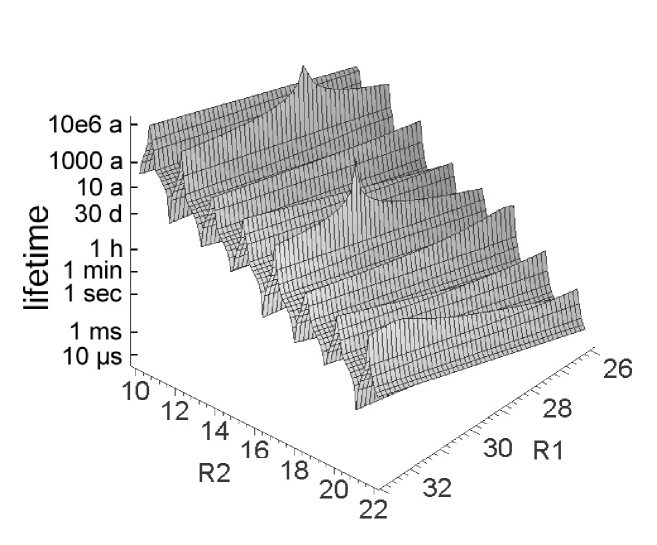
Figure 10: Lifetime $\tau$ (sec, log.scale) as a function of radius $R_{1}$ and $R_{2}$ (in Å) in a 3-dimensional plot. Except for $R_{1}$ and $R_{2}$, all the parameters are chosen as in Fig. 3.

In Fig. 10, the dependence of the lifetime $\tau$ on the radii $R_{1}$ and $R_{2}$ is shown in a 3-dimensional plot. Again one notices that the dependence of $\tau$ on $R_{1}$ is smooth whereas the one on $R_{2}$ contains ”resonances”.

Figure 11: Energy difference between lowest-lying class 1-state and the closest lying class 2-state of the same angular momentum as a function of $R_{2}$ (Å). Energies are given in units of $Ze^{2}_{0}/R_{1}=514.3$ meV. Except for $R_{2}$, all the other parameters are chosen as in Fig. 3.

In Fig. 11, the energy difference between the lowest-lying class 1 state and the closest lying class 2-state of the same angular momentum is shown. The plot supports the explanation of the resonance phenomenon in terms of a coupling between close-lying states.

In the numerical results presented in this section, the values $B$ of the barrier in region I and the well depth $V_{\rm II}$ of the average potential in region II and the dielectric constant $\varepsilon_{\rm I}$ were chosen arbitrarily, and not determined for given choices of the material.

5 Summary and Discussion

In this paper, we determined the quantum states and eigenenergies of an electron in the average potential produced by a positively charged metal cluster which is covered by an insulating surface layer. Because of the similarity of the externally localized electronic states with the bound states of an electron in the Coulomb potential of an atom, we occasionally referred to the system as a ”mesoscopic atom” or, in case of a non-zero total charge, as a ”mesoscopic ion”.

In particular, we investigated the electromagnetic decay of an externally located electron (”class 1-state”) to a lower-lying unoccupied electronic state located within the metal (”class 2-state”). It turned out that the life-time depends sensitively on the radius $R_{2}$ of the metal core and on the number $Z$ of positive surplus charges of the metal. In the model we studied, we found life-times varying between 10^-10 s and years depending on the value of $R_{2}$ or of $Z$.

The value $B$ of the barrier height was 3 eV in our calculations. The lifetime depends strongly on the value of this parameter and decreases for decreasing $B$.

The origin of the large fluctuations was found to be the appearance of states with non-negligible amplitudes both outside and inside of the insulating surface layer (”class 3-states”). The mechanism leading to these ”class 3-states” is described in Appendix.

The wavefunctions and eigenenergies were calculated neglecting the polarization of the insulating surface layer by externally located electrons. The potential produced by these electronic polarization effects was determined in Sec. 3. It was shown that this additional potential matters mainly in the vicinity of the outer surface $S_{1}$ of the insulator and decreases exponentially outside of this surface. The polarization potential could be taken into account by diagonalizing the total Hamiltonian including the polarization potential in the basis of the wavefunctions determined in this paper.

Apart from this physical simplification of the problem we neglected the Coulomb potential produced by the positive surplus charge within the insulator. This approximation is justified whenever the change of the Coulomb potential within the insulating surface layer is much smaller than the barrier height $B_{0}$. This condition was fulfilled in all the cases we studied numerically.

Let us now turn to the discussion of some open questions:

Is the model sufficiently realistic?
Certainly, our model should only be regarded as a first step which has to be improved in various respects.

The 1^st improvement we already mentioned is to incorporate the additional potential between the external electron and the polarization cloud it produces in the insulator. The form of this electronic polarization potential was derived in Sec. 3.

A 2^nd improvement would be to replace the constant potentials $-V^{0}_{\rm II}$ in the metal and $+B_{0}$ in the insulator by periodic potentials defined by the crystal structure of these materials. Of course, this is much more complicated and, to our knowledge, it has rarely been done so far for mesoscopic systems. Furthermore, the crystal structure in mesoscopic aggregates is in general poorly known.

As a result, the electronic eigenvalues of the total system are expected to exhibit a band structure similarly to a macroscopic solid, the insulating surface layer being characterized by a completely filled valence band and an empty conduction band. The empty conduction band in the insulator can be at negative or at positive energy if the energy of the neutral system plus one electron at infinity is put equal to 0. Describing the average potential in the insulator by a positive barrier $B_{0}>0$ is only meaningful if the conduction band of the insulator is at positive energy.

As a further restrictive condition for our model to be a reasonable 1^st approximation there should be no localized traps for an additional electron in the uncharged insulator. This implies that the individual atoms or molecules of the insulator should not have bound states with an additional electron as a monomer [11]. In general, bound states of an electron with a neutral atom or molecule do not exist for atoms or molecules with completely filled shells. Therefore, one should use insulators which exhibit this property. Presumably, Al₂0₃ fulfills this condition. Finally, we neglected effects of the electron-phonon coupling altogether. We presume that they tend to reduce the lifetime, but perhaps not drastically.

What were the physical motivations of this investigation

As long as one can only produce a limited number of ”mesoscopic atoms”, one could just investigate experimentally the effects which we studied in the present paper, especially the amusing strong dependence of the lifetime on the radius and the charge of the metallic core. Although we would be highly pleased by an experimental scrutiny of our predictions, still more exciting open questions could be asked, if it were possible to produce longlived systems of the kind we presented in this paper, and in large quantities. In this case, one would have access to the study of molecules formed from mesoscopic atoms and to condensed matter consisting of mesoscopic atoms as building blocks.

The presence of externally localized electrons would represent a fundamental difference from the case of a condensed system of uncharged mesoscopic clusters. On the one hand, one may expect that, in a condensed matter phase of mesoscopic atoms, the weakly bound external electrons would partly dissociate from their mother atoms and move freely in the average field produced by the charged insulated cores. We would thus surmise that such a system would be a (good) conductor. On the other hand, the fact that the building blocks of such a condensed matter carry charge, will have a profound influence on the equilibrium state of the material. Probably, its density is lower than for uncharged constituents, where the cohesive forces are of van der Waals type and, consequently, of much shorter range.

How far are such dreams from reality?
There are evidently two fundamental obstacles to overcome, a theoretical one and an experimental one.

The theoretical problem is the stability of the charged and insulated single system, and the experimental one is the production of a large number (10²³) of such systems.

As we learnt from this paper, a mesoscopic system of the kind we investigated can only be stable in a strict sense, if there is no empty internally located electronic state below the energy of the lowest externally located state which is at an energy slightly above $-Ze^{2}_{0}/R_{1}$.

The positive surplus charge $Ze_{0}$ on the surface $S_{2}$ of the metal leads to a decrease of the well-depth $V^{0}_{\rm II}\rightarrow V_{\rm II}$ as we have shown in Sec. 3:

$$V_{\rm II}=V^{0}_{\rm II}-{Ze^{2}_{0}\over\varepsilon_{\rm I}}\left({1\over R_{2}}+{\varepsilon_{\rm I}-1\over R_{1}}\right)\,\,.$$ (194)

If, for the uncharged metal, the Fermi level is at the energy $E^{0}_{F}-V^{0}_{\rm II}$ (with $V^{0}_{\rm II}$, $E^{0}_{F}>0$), it lies at the modified energy

$$E^{0}_{F}-V_{\rm II}=E^{0}_{F}-V^{0}_{\rm II}+{Ze^{2}_{0}\over\varepsilon_{\rm I}}\left({1\over R_{2}}+{\varepsilon_{\rm I}-1\over R_{1}}\right)$$ (195)

in the charged metal.

So the condition for strict stability is that there is no level of an internally located electron between $E^{0}_{F}-V_{\rm II}<0$ and $-Ze^{2}_{0}/R_{1}$. As the separation energy $W_{0}>0$ of an electron from the uncharged metal and the Fermi energy $E^{0}_{F}$ are related to $V^{0}_{\rm II}$ by

$$V^{0}_{\rm II}=E^{0}_{F}+W_{0}\,,$$ (196)

we can state that strict stability is achieved whenever there is no level between the energies $-\left\{W_{0}-Ze^{2}_{0}/\varepsilon_{\rm I}\cdot\left[1/R_{2}+(\varepsilon_{\rm I}-1)/R_{1}\right]\right\}$ and $-Ze^{2}_{0}/R_{1}$. This means that, metal with small $W_{0}$ is favourable for stability.

In an ordinary metal, the separation energy $W_{0}$ is of the order of a couple of eV (examples: $W_{0}(\rm Al)=4,28$ eV; $W_{0}(\rm Ag)=4,26$ eV). In the case of a radius $R_{2}=20$ Å of the metal core, the distance between neighbouring electronic levels is of the order of 100 meV. This means that in the case we chose for our numerical investigations, there are many unoccupied levels below the energy of the lowest external electron. However, if we consider a system with an inner radius $R_{2}\approx 4$ Å, the spacing of internally located electron levels of given $l$ approaches already 1 eV. It is therefore conceivable that one might succeed to model a strictly stable ,,mesoscopic atom”.

A further trick to widen the spectrum of internally localized electrons would be to replace the metallic sphere with radius $R_{2}$ by a metallic bubble of outer radius $R_{2}$ and a thickness of 1 Å to 2 Å. In this case the levels differing by the number of radial nodes would have a much larger spacing.

Can such a system be made experimentally?

This is perhaps possible, if one replaces the charged metal layer by a (charged) fullerene $C_{60}$, which has a radius of about 3,5 Å. The separation energy $W_{0}$ of an electron from graphite is known to be $W_{0}=3,8$ eV. We surmise that the separation energy from the fullerene is about the same. Of course, it would no longer be justified to describe free electrons in the fullerene as moving in a simple square well perpendicular to the sphere $S_{2}$. But the spacing of electronic levels is expected to be in the order of eV.

Finally, one is not limited to the spherical geometry. We may also envisage to consider charged nanotubes consisting of a cylindrical surface crystal of $C$-atoms covered by an insulating surface layer. The charge could in this case be generated by applying an external voltage to the ends of the nanotubes. As there is a lot of activity spent on nanotubes presently, we hope that one could succeed to produce small macroscopic amounts of insulated charged nanotubes in a not too far future. Of course, the problem of the stability of externally localized electrons with respect to electromagnetic decay would be similar for nanotubes as for the case of the system we investigated. So we hope that our investigation stimulates the interest of the experts in the field of mesoscopic physics.

Acknowledgement:
Klaus Dietrich gratefully acknowledges the hospitality and support on the occasion of his stay at the Theoretical Physics Institute of the UMCS in April 2003. Krzysztof Pomorski is indebted to the Physics Department of the Technical University of Munich for granting of the honorarium of a visiting professor position in February 2002.

Appendix

Landau-Zener Model for explaining the appearance of class 3-states

Let us consider the simplified potential

$$\widehat{V}(r)=-V_{\rm II}\theta_{0}(R_{2}-r)+B\theta_{0}(R_{1}-r)\theta_{0}(r-R_{2})-{Ze^{2}_{0}\over r}\theta_{0}(r-R_{1})\,\,.$$ (197)

We decompose this potential as follows

$$\widehat{V}(r)=\tilde{V}_{1}(r)+\tilde{V}_{2}(r)\,\,,$$ (198)

$$\widehat{V}_{1}(r)=\theta_{0}(r-R_{1})\left[-B-{Ze^{2}_{0}\over r}\right]\,\,,$$ (199)

$$\widehat{V}_{2}(r)=-V_{\rm II}\theta_{0}(R_{2}-r)+B\theta_{0}(r-R_{2})$$ (200)

and define the two Hamiltonians

$$\widehat{H}_{1(2)}:=\widehat{T}+\widehat{V}_{1(2)}(r)\,\,,$$ (201)

where $\widehat{T}$ is the kinetic energy operator of radial motion

$$\widehat{T}=-{\hbar^{2}\over 2M}\left({d^{2}\over dr^{2}}+{2\over r}{d\over dr}-{l(l+1)\over r^{2}}\right)\,\,.$$ (202)

The eigenstates $\varphi^{(1)}_{\nu}$, $\varphi^{(2)}_{\nu}$ of the Hamiltonians (201)

$$\widehat{H}_{1}\varphi_{\nu}^{(1)}(r)=E^{(1)}_{\nu}\varphi^{(1)}_{\nu}\,\,,$$ (203)

$$\widehat{H}_{2}\varphi_{\nu}^{(2)}(r)=E^{(2)}_{\nu}\varphi^{(2)}_{\nu}$$ (204)

form a non-orthogonal set of basis functions.

We consider an eigenstate $\psi$ of the Hamiltonian $\widehat{H}$ with eigenenergy $E$

$$\widehat{H}:=\widehat{T}+\widehat{V}(r)\,\,,$$ (205)

$$\widehat{H}\psi=E\psi$$ (206)

for the special case that the angular momentum $l$ is the same for all the states and that two specific eigenenergies $E^{(1)}_{\nu}$ and $E^{(2)}_{\nu}$ are very close to the energy $E$ in (206).

Then, we may expect that the expansion of $\psi$ in terms of the basis states $\varphi^{(1)}_{\nu}$ and $\varphi^{(2)}_{\nu}$ may be limited to the two states with the energies $E^{(1)}_{\nu}$, $E^{(2)}_{\nu}$ very close to $E_{\nu}$:

$$|\psi\rangle=A_{\nu}|\varphi^{(1)}_{\nu}\rangle+B_{\nu}|\varphi^{(2)}_{\nu}\rangle\,.$$ (207)

In principle, we would have to sum over all eigenstates $\varphi^{(1)}_{\nu}$ and $\varphi^{(2)}_{\nu}$ on the righthand side of (207), but of all the expansion coefficients $A_{\nu}$, $B_{\nu}$ only the ones corresponding to the energies $E^{(1)}_{\nu}$, $E^{(2)}_{\nu}$ closest to $E$ are expected to be large and all the others to be much smaller.

Henceforth, we leave away the subscript $\nu$ for simplifying the notation. It is convenient to introduce the dual basis states $\tilde{\varphi}^{(1))}$, $\tilde{\varphi}^{(2))}$ defined by the orthogonality conditions

$$\langle\tilde{\varphi}^{(i)}|\varphi^{(j)}\rangle=\delta_{ij}\,\,,$$ (208)

where $i$ and $j$ can be 1 or 2. $\tilde{\varphi}^{(1)}$ and $\tilde{\varphi}^{(2)}$ can be obtained by diagonalizing the inverse of the overlap matrix

$$M^{(ij)}=\langle\varphi^{(i)}|\varphi^{(j)}\rangle\,\,.$$ (209)

It is easily seen that the Schrödinger Eq. (206) together with the assumption (207) leads to the two coupled linear equations

$$\left(\begin{array}[]{cc}(E^{(1)}-E+V^{11}_{2})&V^{12}_{1}\\ V^{21}_{2}&(E^{(2)}-E+V^{22}_{1}\end{array}\right)\left(\begin{array}[]{c}A\\ B\end{array}\right)=0\,\,,$$ (210)

where the matrix elements are defined as follows:

$$V^{ij}_{1,2}:=\langle\tilde{\varphi}^{(i)}|V_{1,2}|\varphi^{(j)}\rangle\,\,.$$ (211)

Introducing the abbreviations

$$\tilde{E}^{(1)}:=E^{(1)}+V^{11}_{2}\,\,,$$ (212)

$$\tilde{E}^{(2)}:=E^{(2)}+V^{22}_{1}$$ (213)

the solutions $E_{\pm}$ of the eigenvalue equation

$$(\tilde{E}^{(1)}-E)(\tilde{E}^{(2)}-E)-V^{12}_{1}\cdot V^{21}_{2}=0$$ (214)

are given by

$$E_{\pm}={\tilde{E}^{(1)}+\tilde{E}^{(2})\over 2}\pm{1\over 2}\sqrt{(\tilde{E}^{(1)}-\tilde{E}^{(2)})^{2}+4V^{12}_{1}V^{21}_{2}}\,\,.$$ (215)

Writing the two states $|\psi\rangle$ in the form

$$|\psi_{\pm}\rangle=A_{\pm}\cdot\left\{|\varphi^{(1)}\rangle\pm\lambda_{\pm}|\varphi^{(2)}\rangle\right\}\,\,,$$ (216)

where

$$\lambda_{\pm}:={B_{\pm}\over A_{\pm}}\,\,,$$ (217)

one obtains $\lambda$ from the Eq. (210) and the amplitudes $A_{\pm}$ from the normalisation of $|\psi_{\pm}\rangle$.

The physically interesting quantities are the probabilities $W^{(1,2)}_{+}$ and $W^{(1,2)}_{-}$ to find the system described by $|\psi_{\pm}\rangle$ in the substate $\varphi^{(1)}$ or $\varphi^{(2)}$. These probabilities are given by the mean-values of the projection operators

$$\widehat{P}_{(1,2)}:=|\varphi^{(1,2)}\rangle\langle\tilde{\varphi}^{(1,2)}|\,\,.$$ (218)

It is easily seen that the probabilities are given by the following equations

$$W^{(1)}_{+}=\langle\psi_{+}|\widehat{P}_{(1)}|\psi_{+}\rangle={1+\lambda_{+}M^{12}\over 1+2\lambda_{+}M^{12}+\lambda_{+}^{2}}\,\,,$$ (219)

$$W^{(2)}_{+}=\langle\psi_{+}|\widehat{P}_{(2)}|\psi_{+}\rangle={\lambda_{+}(\lambda_{+}+M^{12})\over 1+2\lambda_{+}M^{12}+\lambda_{+}^{2}}\,\,,$$ (220)

$$W^{(1)}_{-}=\langle\psi_{-}|\widehat{P}_{(1)}|\psi_{-}\rangle={1-\lambda_{-}M^{12}\over 1-2\lambda_{-}M^{12}+\lambda_{-}^{2}}\,\,,$$ (221)

$$W^{(2)}_{-}=\langle\psi_{-}|\widehat{P}_{(2)}|\psi_{-}\rangle={\lambda_{-}(\lambda_{-}-M^{12})\over 1-2\lambda_{-}M^{12}+\lambda_{-}^{2}}\,\,,$$ (222)

where $M^{12}$ is the overlap of the two basis states

$$M^{12}=\langle\varphi^{(1)}|\varphi^{(2)}\rangle$$ (223)

and the quantities $\lambda_{\pm}$ by

$$\lambda_{\pm}={1\over 2V^{12}}\left\{-\Delta E^{(1,2)}\pm\sqrt{(\Delta E^{(1,2)})^{2}+4V^{12}_{1}V^{21}_{2}}\right\}\,\,,$$ (224)

where

$$\Delta E:=E^{(1)}-E^{(2)}\,.$$ (225)

It is seen that for

$$|\Delta E|^{2}\gg 4|V^{12}_{1}\cdot V^{21}_{2}|\,\,,$$ (226)

i.e. far away from the crossing of the energies $E^{(1)}$ and $E^{(2)}$, one of the ratios $\lambda_{\pm}$ is much larger than the other.

Figure 12: Schematic plot of the Landau-Zener crossing of an external and an internal energy $E^{(1,2)}$ yielding the class 3-state energies $E_{\pm}$.

For $\Delta E>0$ one finds

$$\lambda_{+}\approx{V^{21}_{2}\over\Delta E}\,\,,$$ (227)

$$\lambda_{-}\approx-\left[{\Delta E\over V^{12}_{1}}+{V^{21}_{2}\over\Delta E}\right]$$ (228)

and for $\Delta E<0$ the reversed result

$$\lambda_{+}\approx{\Delta E\over V^{12}_{1}}+{V^{21}_{2}\over|\Delta E|}\,\,,$$ (229)

$$\lambda_{-}\approx-{V^{21}_{2}\over|\Delta E|}\,.$$ (230)

This shows that a predominantly externally localized state turns into a predominantly internally localized one as the energies $E^{(1)}$ and $E^{(2)}$ cross as a function of $R_{2}$ or $Z$. The coupled true states $\psi_{\pm}$ are thus seen to change their nature as a result of the crossing of the energies $E^{(1)}$, $E^{(2)}$ of a class 1 and a class 2 state. Close to the crossing point the states $\psi_{\pm}$ are seen to be ”delocalized”, containing comparable contributions of the two basis states $\varphi^{(1,2)}$.

This is in essence a Landau-Zener crossing. In Fig. 12 we show a schematic picture of the energies $E^{(1)}$, $E^{(2)}$, $E_{+}$, and $E_{-}$ as a function of the the parameter $R_{2}$ or $Z$.

References

- [1] W. D. Knight, K. Clemenger, W. A. de Heer, W. A. Saunders, M. Y. Chou, M. L. Cohen: Phys. Rev. Lett. 52, (1984) 2141; W. D. Knight, W. A. de Heer, K. Clemenger, W. A. Saunders: Solid State Commun. 53, (1985) 44; Hellmut Haberland (ed): “Clusters of Atoms and Molecules”, vol. 1 and 2, Springer Verlag, 1994.
- [2] S. Frank, N. Malinowski, F. Tast, M. Heinebrodt, I.M.L. Billas, T.P. Martin: Z. Phys. D40, (1997) 250; M. Springborg, S. Satpathy, N. Malinowski, T.P. Martin, U. Zimmermann: Phys. Rev. Lett. 77, (1996) 1127; H. Kuzmany, J. Fink, M. Mehring, S. Roth (eds): “Electronic Properties of Fullerenes”, Springer-Verlag, 1993.
- [3] M. Brack: Rev. Mod. Phys. 65, 677 (1993).
- [4] W. A. de Heer, Rev. Mod. Phys. 65, 611 (1993).
- [5] M. Abramowitz and J.A. Stegun (eds): “Handbook of Mathematical Functions”, Nat. Bureau of Standards, Applied Mathematics, Series 55, issued June 1964.
- [6] A. Erdelyi, “Higher Transcendental Functions”, McGraw-Hill, 1953.
- [7] J.D. Jackson: “Classical Electrodynamics”, John Wiley, 1967.
- [8] B.H. Bransden and C.J. Joachain, “Physics of Atoms and Molecules”, Longman Group Limited, 1983.
- [9] M.E. Rose, “ Elementary Theory of Angular Momentum”, New York: Dover, 1995
- [10] L.D. Landau, Phys. Z. Sov. 2 (1932) 46; C. Zener, Proc. Roy. Soc. (London) A137 (1932) 696.
- [11] H. Haberland and K.H. Bowen: “Solvated Electron Clusters”, Chapt. 2.5 in “Cluster of Atoms and Molecules II”, vol. 56 of the Springer Series in Chemical Physics, 1994.