Fluctuation induced effects in confined electrolyte solutions

Abstract

We examine electrolyte systems confined between two parallel, grounded metal plates using a field-theoretic approach truncated at one-loop order. For symmetric electrolytes, the system is locally neutral, and the electric potential between the plates is everywhere zero, in agreement with the predictions of the Poisson-Boltzmann equation. The density distribution of the ions, however, is non-uniform, with a maximum value at the center of the system and that lies below the bulk electrolyte density. This differs from the Poisson-Boltzmann result, which is uniform and equal to the bulk electrolyte density. For asymmetric electrolytes, the system is no longer locally neutral, and there is a non-zero static electric potential. In addition, the surface of the metal plates becomes charged. When the plate separation is smaller than the screening length, the charge distribution has a single peak at the center of the system. As the separation becomes greater than the screening length, the charge distribution possesses two peaks with a local minimum at the center of the system. These peaks remain localized near the surface of the plates, while the bulk of the system has nearly zero charge. When the plates are immersed in a bulk electrolyte solution, an attractive fluctation induced force develops between them that is analogous to the Casimir force. Unlike the Casimir force, however, this attractive interaction has a finite limit in the zero separation limit and decays inversely with the separation at large separations.

I Introduction

The electrical double layer near a solid/electrolyte interface occurs in a wide variety of contexts and plays a crucial role in many colloidal, electrochemical, and biological systems. Much of our understanding of these systems are based on the Poisson-Boltzmann equation, which has been quite successful Gouy_1910 ; Chapman_1913 ; Israelachvili_1991 . This equation is based on a mean-field type approximation, and, consequently, neglects fluctuation effects which result in ion-ion correlations. In many cases, these fluctuations are not crucial, and only add a qualitative change in the predictions.

In certain situations, however, the contribution of fluctuations are important and lead to qualitatively different behavior than that predicted by the Poisson-Boltzmann equation Levin_2002 . Examples include the presence of an attractive interaction between two like-charged colloids Wu_etal_1999 ; Moreira_Netz_2001 , the collapse of polyelectrolytes Golestanian_etal_1999 , and charge segregation in confined electrolytes Yu_etal_1997 ; Sheng_Tsao_2002 .

Due to the importance of fluctuations, many theoretical methods have been developed to incorporate fluctuation corrections in electrolyte systems. Some of these include liquid-state theory approaches based on the Ornstein-Zernike equation coupled with an approximation closure, such as the hypernetted-chain or mean-spherical approximation Henderson_Blum_1978 ; Kjellander_Marcelja_1985 ; Attard_etal_1988a ; Attard_etal_1988b , density functional theories Biben_etal_1998 ; Boda_etal_1999 ; Boda_etal_2002 , the modified Poisson-Boltzmann equation Outhwaite_etal_1980 , computer simulation methods Torrie_Valleau_1980 ; Torrie_etal_1982 ; Boda_etal_1999 ; Boda_etal_2002 , and field theoretic approaches Kholodenko_Beyerlein_1986 ; Ortner_1999 ; Netz_Orland_2000b ; Brown_Yaffe_2001 .

We examine a pair of grounded, metal plates which are separated by a distance $L$ and immersed in an electrolyte solution which is dissolved in a continuum with uniform dielectric constant $\epsilon$. In this situation, the Poisson-Boltzmann equation predicts that the system behaves trivially: the ion concentration between the plates is uniform, and the electric potential is everywhere zero. For this system, the fluctuation corrections are non-trivial and lead to some interesting phenomena. In this case, the ion concentration is non-uniform, and in some situations can lead to the presence of a non-zero electric potential and a surface charge on the metal plates. In addition, we find a fluctuation induced attractive force, analogous to the Casimir force, between metal plates.

The remainder of the paper is organized as follows. In Section II, we quickly review the functional integral formulation of electrolyte systems. Then in Section III, we quickly summarize the main results in mean-field theory (i.e., the Poisson-Boltzmann equation) for electrolytes confined between two metal plates and then present field theory calculations to order one-loop. Finally, in Section IV we summarize the major finding in this work.

II Functional integral formulation

Consider an electrolyte system that is immersed in a continuous medium with a uniform dielectric constant $\epsilon$ and is composed of point charges. The charge density $Q({\bf r})$ in the system is given by

$$Q({\bf r}) = \sum_{\alpha,k}q_{\alpha}\delta({\bf r}-{\bf r}_{\alpha,k})+\Sigma({\bf r})$$ (1)

where $r_{\alpha,k}$ is the position of the $k$th particle of type $\alpha$, and $\Sigma({\bf r})$ is an applied charge density.

The total electrostatic energy $E$ of the system is given by Jackson_1975

$$E = \frac{\epsilon}{8\pi}\int d{\bf r}\nabla\phi({\bf r})\cdot\nabla\phi({\bf r})$$ (2)

where $\phi$ is the electrostatic potential, which can be obtained by solving Poisson’s equation

$$-\epsilon\nabla^{2}\phi({\bf r}) = 4\pi Q({\bf r})$$ (3)

where $\phi$ is the electrostatic potential, and $Q({\bf r})$ is the charge density.

The associated Green’s function to this problem is:

$$-\frac{\epsilon}{4\pi}\nabla^{2}G_{0}({\bf r},{\bf r}^{\prime}) = \delta({\bf r}-{\bf r}^{\prime})$$ (4)

where $G_{0}({\bf r},{\bf r}^{\prime})$ is the Green’s function. Given the Green’s function, the electrostatic potential can be determine directly from the charge density distribution $Q({\bf r})$ in the system Jackson_1975 :

$$\phi({\bf r}) = \int d{\bf r}^{\prime}G_{0}({\bf r}^{\prime},{\bf r})Q({\bf r}^{\prime})$$ (5)

$$\quad+\frac{\epsilon}{4\pi}\oint d{\bf r}^{\prime}[G_{0}({\bf r}^{\prime},{\bf r})\nabla^{\prime}\phi({\bf r}^{\prime})$$

$$\quad-\phi({\bf r}^{\prime})\nabla^{\prime}G_{0}({\bf r}^{\prime},{\bf r})]$$

where the surface integral is taken over the boundary of the system, with the vector $d{\bf r}^{\prime}$ pointing outwards from the system, normal to its surface. The second term depends only on the boundary conditions of the system and not on the charge distribution within the system.

For the problem of an electrolyte confined between two metal plates, we have Dirichlet boundary conditions and the potential $\phi$ is zero on the metal surface. In this situation, we choose $G_{0}({\bf r}^{\prime},{\bf r})=0$ for ${\bf r}^{\prime}$ on the surface, and so the surface terms in Eq. (5) vanish to yield:

$$\phi({\bf r}) = \int d{\bf r}^{\prime}G_{0}({\bf r},{\bf r}^{\prime})Q({\bf r}^{\prime})$$ (6)

The energy of the electrostatic field can then be written entirely in terms of the charge distribution

$$E = \frac{1}{2}\int d{\bf r}d{\bf r}^{\prime}Q({\bf r})G_{0}({\bf r},{\bf r}^{\prime})Q({\bf r}^{\prime})$$ (7)

The expression for the energy given above contains contribution from the interaction of each ion with itself — the self-energy. Subtracting this term from the energy, we write

$$E = \frac{1}{2}\int d{\bf r}dr^{\prime}Q({\bf r})G_{0}({\bf r},{\bf r}^{\prime})Q({\bf r}^{\prime})$$ (8)

$$\qquad-\frac{1}{2}\sum_{\alpha,k}q_{\alpha}^{2}G_{0}({\bf r}_{\alpha,k},{\bf r}_{\alpha,k})$$

The grand partition function $Z_{G}$ for a system of point charges at fixed chemical potential $\mu_{\alpha}$ is given by

$$Z_{G}[\gamma] = \sum_{N_{1}=0}^{\infty}\cdots\sum_{N_{M}=0}^{\infty}\prod_{\nu}\frac{1}{N_{\nu}!\Lambda_{\nu}^{3N_{\nu}}}$$ (9)

$$\qquad\times\int\prod_{\tau t}d{\bf r}_{\tau t}e^{-\beta E+\sum_{\alpha,k}\gamma_{\alpha}({\bf r}_{\alpha,k})}$$

$$= \sum_{N_{1}=0}^{\infty}\cdots\sum_{N_{M}=0}^{\infty}\prod_{\nu}\frac{1}{N_{\nu}!\Lambda_{\nu}^{3N_{\nu}}}\int\prod_{\tau t}d{\bf r}_{\tau t}$$

$$\qquad\times e^{-\frac{\beta}{2}\int d{\bf r}d{\bf r}^{\prime}Q({\bf r})G_{0}({\bf r},{\bf r}^{\prime})Q({\bf r}^{\prime})}$$

$$\qquad\times e^{\sum_{\alpha,k}[\gamma_{\alpha}({\bf r}_{\alpha,k})+\frac{\beta}{2}q_{\alpha}^{2}G_{0}({\bf r}_{\alpha,k},{\bf r}_{\alpha,k})]}$$

where $\beta=1/(k_{B}T)$, $k_{B}$ is the Boltzmann constant, $N_{\nu}$ is the number of ions of type $\nu$, ${\bf r}_{\alpha j}$ is the position of the $j$th ion of type $\alpha$, $\Lambda_{\nu}$ is the thermal wavelength of an ion of type $\nu$, $\gamma_{\alpha}({\bf r})=\beta[\mu_{\alpha}+u_{\alpha}({\bf r})]$, and $u_{\alpha}$ is an external potential acting on ions of type $\alpha$.

Introducing the Hubbard-Stratonovich transformation, the grand partition function can be expressed in terms of a functional integral Kholodenko_Beyerlein_1986 ; Lue_etal_1999 ; Ortner_1999 ; Netz_Orland_2000b

$$Z_{G}[\gamma] = \frac{1}{{\mathcal{N}}_{0}}\int{\mathcal{D}}\psi(\cdot)$$ (10)

$$\quad\times\exp\Bigg{[}-\frac{1}{2\beta}\int d{\bf r}d{\bf r}^{\prime}\psi({\bf r})G_{0}^{-1}({\bf r},{\bf r}^{\prime})\psi({\bf r}^{\prime})$$

$$\quad+\sum_{\alpha}\Lambda_{\alpha}^{-d}\int d{\bf r}e^{\gamma_{\alpha}({\bf r})-q_{\alpha}i\psi({\bf r})}$$

$$\quad\times e^{\frac{1}{2}\beta q_{\alpha}^{2}G_{0}({\bf r},{\bf r})}\Bigg{]}$$

where

$${\mathcal{N}}_{0} = \int{\mathcal{D}}\psi(\cdot)\exp\left[-\frac{1}{2\beta}\int d{\bf r}d{\bf r}^{\prime}\psi({\bf r})G_{0}^{-1}({\bf r},{\bf r}^{\prime})\psi({\bf r}^{\prime})\right].$$ (11)

The function $i\psi({\bf r})$ can be interpreted as being equal to an instantaneous value of $\beta\phi({\bf r})$, and the functional integral can be thought of as an integral over all possible “shapes” of the electric field due to the thermal motion of the electrolytes.

II.1 Mean-field approximation

In the mean-field approximation, the value of the functional integral is replaced by the value of the integrand at its saddle point. The value of the field at the saddle point, denoted by $\bar{\psi}$, is given implicitly by

$$\frac{\delta\ln Z_{G}[i\bar{\psi}]}{\delta i\psi(r)} = 0,$$

which leads to the relation

$$-\frac{\epsilon}{4\pi\beta}\nabla^{2}i\bar{\psi}({\bf r}) = \sum_{\alpha}q_{\alpha}\Lambda_{\alpha}^{-d}e^{\gamma_{\alpha}({\bf r})-q_{\alpha}i\bar{\psi}({\bf r})}$$ (12)

$$\qquad+\Sigma({\bf r}).$$

This is precisely the Poisson-Boltzmann equation. The electric potential is given by $\phi({\bf r})=k_{B}Ti\bar{\psi}({\bf r})$.

Within the mean-field approximation, the grand potential is given by

$$\ln\bar{Z}_{G}[\gamma] = \frac{1}{2\beta}\int d{\bf r}d{\bf r}^{\prime}i\bar{\psi}({\bf r})G_{0}^{-1}({\bf r},{\bf r}^{\prime})i\bar{\psi}({\bf r}^{\prime})$$ (13)

$$\quad+\sum_{\alpha}\Lambda_{\alpha}^{-d}\int d{\bf r}e^{\gamma_{\alpha}({\bf r})-q_{\alpha}i\bar{\psi}({\bf r})}$$

The density distribution of ion of species $\alpha$ can be determined by taking the functional derivative of the grand partition function with respect to $\gamma_{\alpha}$ Lebowitz_Percus_1963 , which yields

$$\bar{\rho}_{\alpha}({\bf r}) = \frac{\delta\ln\bar{Z}_{G}[\gamma]}{\delta\gamma_{\alpha}({\bf r})}$$ (14)

$$= \Lambda_{\alpha}^{-d}e^{\gamma_{\alpha}({\bf r})-q_{\alpha}i\bar{\psi}({\bf r})}$$

II.2 One-loop expansion

The functional integral for the grand partition function can be cast into a form that allows one to perform a loop-wise expansion around the mean-field solution $\bar{\psi}({\bf r})$. Defining $\delta\psi=\psi-\bar{\psi}$ as the deviation from the mean-field solution, Eq. (10) is re-written as a functional integral over $\delta\psi({\bf r})$. The quadratic term in the action is now defined by a screened propagator (Green’ s function) defined by a Dyson equation

$$G^{-1}({\bf r},{\bf r}^{\prime}) = G_{0}^{-1}({\bf r},{\bf r}^{\prime})+\delta({\bf r}-{\bf r}^{\prime})\bar{K}_{2}({\bf r}^{\prime}),$$ (15)

where the $n$-th moments of the mean-field charge densities have been defined as

$$\bar{K}_{n}({\bf r}) \equiv \beta\sum_{\alpha}q_{\alpha}^{n}\bar{\rho}_{\alpha}({\bf r}).$$ (16)

The second moment $\bar{K}_{2}({\bf r})$ corresponds to a (in general ${\bf r}$-dependent) inverse screening length. The third moment $\bar{K}_{3}({\bf r})$ will turn out to be crucial for the physics of asymmetric electrolytes. Expanding to order one-loop,

$$\ln Z_{G}^{(1)}[\gamma] = \ln\bar{Z}_{G}[\gamma]$$

$$- \frac{1}{2}{\rm Tr}[\ln(1+\bar{K}_{2}G_{0})-\bar{K}_{2}G_{0}].$$

Here, the last term $\frac{1}{2}{\rm Tr}[\bar{K}_{2}G_{0}]$ corresponds to the self-energy of the charges which has to be subtracted from the total electrostatic energy. Equation (II.2), which is still completely general, forms the starting point for the discussion of fluctuation-induced effects in electrolytes. Since in the following, all the calculations are to one-loop order, the index $(1)$ in $Z_{G}^{(1)}$ is omitted.

III Conducting parallel plates

Consider a medium of dielectric constant $\epsilon$ which is confined between two conducting metal plates separated by a distance $L$. In this geometry, the mean-field solution for the field $\bar{\psi}({\bf r})$ and the densities $\bar{\rho}_{\alpha}({\bf r})$ is trivial,

$$i\bar{\psi}({\bf r}) = 0,\quad\bar{\rho}_{\alpha}({\bf r})=\bar{\rho}_{\alpha}=\Lambda_{\alpha}^{-d}e^{\gamma_{\alpha}}.$$ (18)

That is, the electric potential between the plates is zero, and the electrolyte density is uniform and solely determined by the chemical potentials $\mu_{\alpha}$ and the temperature $k_{B}T=1/\beta$ ($\gamma_{\alpha}=\beta\mu_{\alpha}$).

The (screened) Green’s function $G({\bf r},{\bf r}^{\prime})$ for the Poisson-Boltzmann equation is obtained from a Fourier series for the screened Coulomb interaction and given by

$$G({\bf r},{\bf r}^{\prime}) = \frac{4\pi}{\epsilon}\frac{2}{L}\sum_{n=1}^{\infty}\int\frac{dq_{1}}{2\pi}\frac{dq_{2}}{2\pi}\left[\left(\frac{n\pi}{L}\right)^{2}+q_{1}^{2}+q_{2}^{2}+\kappa^{2}\right]^{-1}\sin\left(\frac{n\pi z}{L}\right)\sin\left(\frac{n\pi z^{\prime}}{L}\right)e^{iq_{1}(x-x^{\prime})+iq_{2}(y-y^{\prime})},$$ (19)

where $\kappa$ is the inverse Debye screening length in the mean-field approximation, which is defined as

$$\kappa^{2} \equiv \frac{4\pi}{\epsilon}\bar{K}_{2}=\frac{4\pi\beta}{\epsilon}\sum_{\alpha}q_{\alpha}^{2}\bar{\rho}_{\alpha}$$ (20)

The (unscreened) Green’s function $G_{0}({\bf r},{\bf r}^{\prime})$ of the Poisson equation (see Eqs. (3) and (4)), is obtained from Eq. (19) by setting $\kappa=0$.

III.1 Density profile

All the thermodynamic properties of the system can be derived from the grand potential. The density profile to one loop order is given by the functional derivative Lebowitz_Percus_1963

$$\rho_{\alpha}({\bf r}) = \frac{\delta\ln Z_{G}}{\delta\gamma_{\alpha}({\bf r})}\approx\bar{\rho}_{\alpha}\left[1-\frac{\beta q_{\alpha}^{2}}{2}\Delta G({\bf r},{\bf r})\right.$$

$$\qquad\left.+\frac{\beta q_{\alpha}}{2}\int d{\bf r}^{\prime}\Delta G({\bf r}^{\prime},{\bf r}^{\prime})\bar{K}_{3}({\bf r}^{\prime})G({\bf r}^{\prime},{\bf r})\right],$$

where

$$\Delta G({\bf r},{\bf r}) \equiv G({\bf r},{\bf r})-G_{0}({\bf r},{\bf r})=-\frac{2}{\epsilon L}I_{1}(\kappa L,z)$$ (22)

with $I_{1}$ defined as

$$I_{1}(\kappa L,z) \equiv \sum_{n=1}^{\infty}\sin^{2}\left(\frac{n\pi z}{L}\right)\ln\left(1+\left(\frac{\kappa L}{n\pi}\right)^{2}\right)$$ (23)

Note that in the bulk limit where $L\to\infty$, $G({\bf r},{\bf r}^{\prime})=e^{-\kappa|{\bf r}-{\bf r}^{\prime}|}/(\epsilon|{\bf r}-{\bf r}^{\prime}|)$, and $\Delta G(r,r)=-\kappa/\epsilon$. In this case, the density profile becomes uniform and is given by

$$\rho_{\alpha}^{\rm bulk} \approx \Lambda_{\alpha}^{-d}e^{\gamma_{\alpha}}\left[1+\frac{\beta q_{\alpha}^{2}\kappa}{2\epsilon}-\frac{4\pi\beta q_{\alpha}}{2\epsilon\kappa}\bar{K}_{3}\right]$$ (24)

For symmetric electrolytes, where the magnitude of all the charges of the particles is the same (i.e., $|q_{\alpha}|=q$ for all $\alpha$, and therefore $\bar{K}_{3}=0$), the last term in Eq. (III.1) vanishes, and the expression for the density profile reduces to

$$\rho_{\alpha}({\bf r}) \approx \Lambda_{\alpha}^{-d}e^{\gamma_{\alpha}}\left[1+\frac{\beta q_{\alpha}^{2}}{\epsilon L}I_{1}(\kappa L,z)\right]$$ (25)

The second term is the only correction term for a symmetric electrolyte, and its sign is independent of the sign of the charge. As a result, the fluctuation corrections increase the electrolyte concentration of the system, as compared to the mean-field approximation. However, the ion concentration at the metal surface remains at its mean-field value. In addition, the system is everywhere locally neutral.

The difference between the density between the plates and that of a bulk system at the same chemical potential is given by

$$\rho_{\alpha}({\bf r})-\rho_{\alpha}^{\rm bulk} \approx \frac{\beta\bar{\rho}_{\alpha}q_{\alpha}^{2}}{\epsilon L}\left[I_{1}(\kappa L,z)-\frac{\kappa L}{2}\right]$$ (26)

Plots of the density profile difference between the confined system and the bulk system at different values of $\kappa L$ are given in Fig. 1. In Fig. 1a, the plate separation $L$ is varied while holding the value of $\kappa$ (i.e., the ion chemical potentials) fixed; in Fig. 1b, the value of $\kappa$ is varied while the plate separation is held fixed.

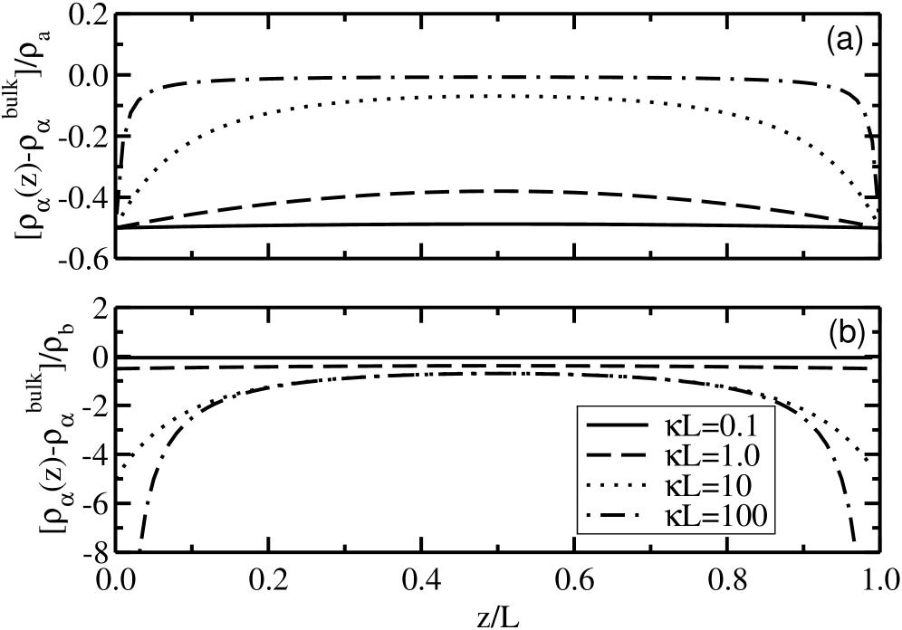
Figure 1: Density profile for a symmetric electrolyte solution confined between two conducting plates with (a) $\kappa$ held constant ($\rho_{a}=\beta\bar{\rho}_{\alpha}q_{\alpha}^{2}\kappa/\epsilon$) and with (b) $L$ held constant ($\rho_{b}=\beta\bar{\rho}_{\alpha}q_{\alpha}^{2}/(\epsilon L)$): (i) $\kappa L=0.1$ (solid line), (ii) $\kappa L=1$ (dashed line), (iii) $\kappa L=10$ (dotted line), and (iv) $\kappa L=100$ (dashed-dotted line).

The ions are more concentrated in the center of the system than near the plates. At the center of the plates, where the ion concentration is at a maximum, the density can be computed in closed form, to yield:

$$\rho_{\alpha}\left(\frac{L}{2}\right) = \bar{\rho}_{\alpha}\left[1+\frac{\beta q_{\alpha}^{2}}{\epsilon L}\ln\cosh\frac{\kappa L}{2}\right]$$ (27)

In addition, for a symmetric electrolyte, the concentration of the ions in the confined system is lower than that of the bulk system at the same chemical potentials.

The local charge distribution $Q({\bf r})$ between the plates can be computed from the density distribution of the ions:

$$Q({\bf r}) \equiv \sum_{\alpha}q_{\alpha}\rho_{\alpha}({\bf r})$$

$$= -\frac{\bar{K}_{3}}{2}\left\{\Delta G({\bf r},{\bf r})-\bar{K}_{2}\int d{\bf r}^{\prime}\Delta G({\bf r}^{\prime},{\bf r}^{\prime})G({\bf r}^{\prime},{\bf r})\right\}$$

$$= \frac{2\sigma^{*}}{L}\Bigg{\{}I_{1}(\kappa L,z)-(\kappa L)^{2}I_{2}(\kappa L,z)$$

$$\qquad+\frac{\sinh\frac{\kappa z}{2}\sinh\frac{\kappa L}{2}(z/L-1)}{\cosh\frac{\kappa L}{2}}(\kappa L)^{2}I_{3}(\kappa L)\Bigg{\}},$$

where we have used the fact that $\sum_{\alpha}q_{\alpha}\bar{\rho}_{\alpha}=0$, defined $\sigma^{*}\equiv\bar{K}_{3}/(2\epsilon)$, and introduced the functions (cf. Appendix A)

$$I_{2}(\kappa L,z) = \sum_{m=1}^{\infty}\frac{\ln\left(1+\left(\frac{\kappa L}{m\pi}\right)^{2}\right)}{(2m\pi)^{2}+(\kappa L)^{2}}\sin^{2}\frac{m\pi z}{L}$$ (29)

$$I_{3}(\kappa L) = \frac{1}{(\kappa L)^{2}}\sum_{m=1}^{\infty}\frac{(2m\pi)^{2}\ln\left(1+\left(\frac{\kappa L}{m\pi}\right)^{2}\right)}{(2m\pi)^{2}+(\kappa L)^{2}}.$$

In the case where $\bar{K}_{3}=0$ (e.g., a symmetric electrolyte with $|q_{\alpha}|=q$ for all $\alpha$), $Q({\bf r})$ is trivially zero, and the system (apart from being locally neutral everywhere) is globally neutral.

A non-trivial situation arises for asymmetric electrolytes with $\bar{K}_{3}\neq 0$. As shown below, the fluctuations around the mean-field solution lead to a non-zero charge distribution between the metal plates with a density profile that strongly depends on the dimensionless parameter $\kappa L$.

In Fig. 2, the variation of the local charge distribution for different values of $\kappa L$ is plotted at constant $\kappa$. For low values of $\kappa L$, the local charge distribution has a single peak located in the center of the system with the same sign as $\bar{K}_{3}$. For a binary asymmetric electrolyte, this implies that the sign of the net local charge is the same as that of the ion with the larger charge magnitude.

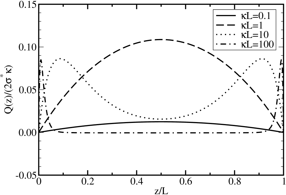
Figure 2: Variation of the charge density for an electrolyte solution confined between two conducting plates at constant $\kappa$: (i) $\kappa L=0.1$ (solid line), (ii) $\kappa L=1$ (dashed line), (iii) $\kappa L=10$ (dotted line), and (iv) $\kappa L=100$ (dashed-dotted line).

As $\kappa L$ further increases, the charge distribution initially uniformly increases; however, at a critical value of $\kappa L$, the single peak becomes a local minimum, and two peaks emerge on either side of this minimum. These peaks move towards the boundaries with increasing $\kappa L$, while the value of the charge density at the center of the system decreases, eventually changing sign. This is similar to the change in the monomer distribution for a polyelectrolyte confined between two oppositely charged plates Podgornik_Dobnikar_2001 .

As the plates become further and further separated, the charge density near the plates approaches a limiting form $Q_{\infty}(z)\equiv\lim_{\kappa L\to\infty}Q(z)/(2\kappa\sigma^{*})$, which can be written analytically as:

$$Q_{\infty}(z) = \frac{1}{4\kappa z}(e^{-2\kappa z}-1)+\left(\frac{1}{2}-\frac{\log 3}{8}\right)e^{-\kappa z}$$

$$\quad+\frac{e^{\kappa z}}{8}\left[\mbox{\rm Ei}(-3\kappa z)-\mbox{\rm Ei}(-\kappa z)\right]$$

$$\quad-\frac{e^{-\kappa z}}{8}\left[\mbox{\rm Ei}(-\kappa z)-\mbox{\rm Ei}(\kappa z)\right]$$

where ${\rm Ei}$ denotes the exponential integral. This function is plotted in Fig. 3.

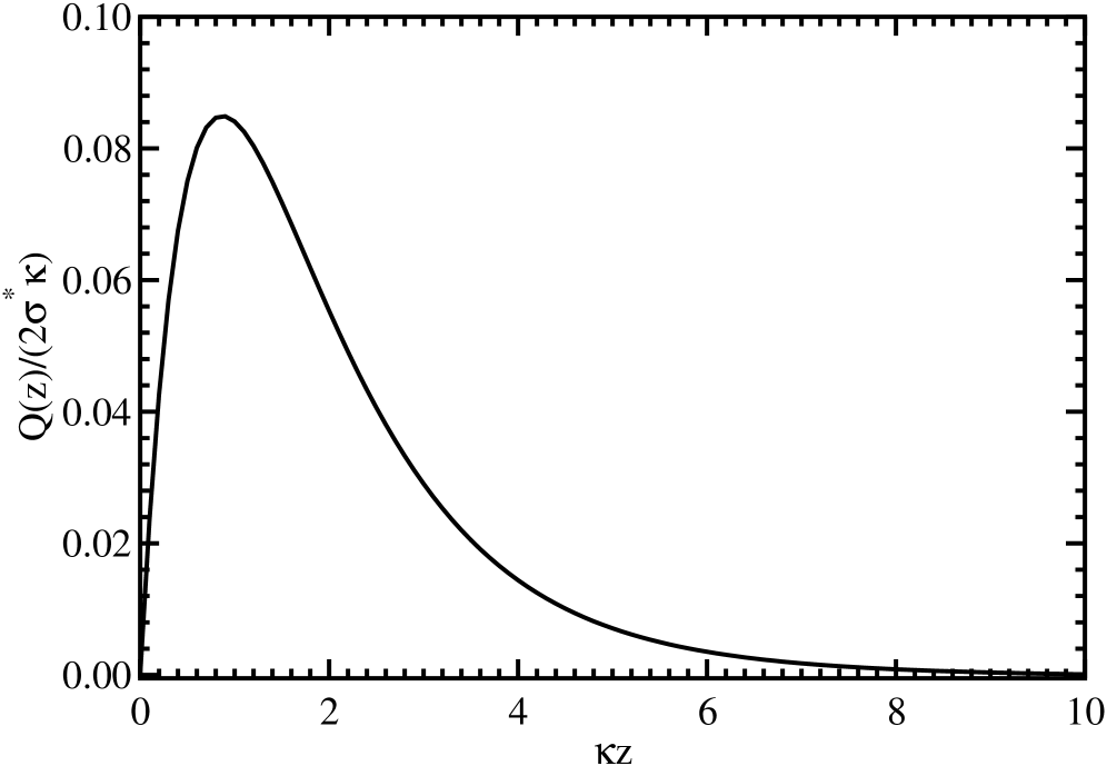
Figure 3: The local charge distribution near a metal plate in the limit of infinite plate separation.

Integrating the distribution of charge contained between the plates, the total net charge per unit area ${\mathcal{Q}}$ is determined to be

$${\mathcal{Q}} = \int_{0}^{L}dzQ({\bf r})=2\sigma^{*}(\kappa L)\tanh\frac{\kappa L}{2}I_{3}(\kappa L).$$ (31)

Therefore, an asymmetric electrolyte system has a non-vanishing net charge. As shown in the next section, this net charge is counter-balanced by an induced surface charge on the metal plates.

III.2 Electric potential

The electric potential $\phi({\bf r})$ between the plates can be obtained from the grand partition function Netz_Orland_2000b

$$\phi({\bf r}) = \frac{1}{\beta}i\psi({\bf r})=\frac{1}{\beta}\frac{\delta\ln Z_{G}}{\delta\Sigma({\bf r})}$$ (32)

$$\approx -\frac{\bar{K}_{3}}{2}\int dr^{\prime}\Delta G(r^{\prime},r^{\prime})G(r^{\prime},r)$$

$$\approx -\frac{8\pi\sigma^{*}L}{\epsilon}\Bigg{[}\frac{\sinh\frac{\kappa z}{2}\sinh\frac{\kappa L}{2}(z/L-1)}{\cosh\frac{\kappa L}{2}}I_{3}(\kappa L)$$

$$\qquad-I_{2}(\kappa L,z)\Bigg{]}$$

In the case of a symmetric electrolyte, the correction term vanishes, and the electric field is identically zero between the plates, similar to the mean-field approximation. In the case of an asymmetric electrolyte, however, the fluctuation correction is non-zero, and the electric potential varies within the cavity.

In Fig. 4, the electric potential $\phi(z)$ in the system is plotted. If the plate distance is kept fixed, then the electric potential between the plates uniformly increases with $\kappa$ to a constant profile (see Fig. 4a). If $\kappa$ is held fixed while the distance between the plates $L$ is increased, then the potential increases from zero to a maximum value at a critical value of $L$, and subsequently decrease to zero (see Fig. 4b).

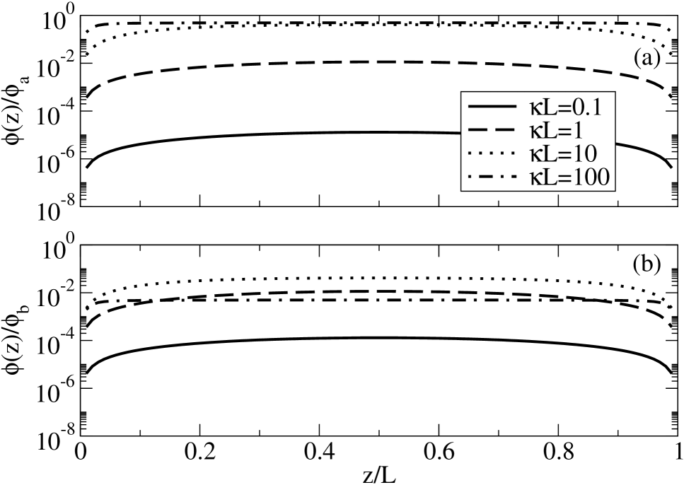
Figure 4: Variation of the electric potential between the metal plates at (a) fixed $\kappa$ ($\phi_{a}=-8\pi\sigma^{*}/(\epsilon\kappa)$) and (b) fixed plate separation $L$ ($\phi_{b}=-8\pi\sigma^{*}L/\epsilon$): (i) $\kappa L=0.1$ (solid line), (ii) $\kappa L=1$ (dashed line), (iii) $\kappa L=10$ (dotted line), and (iv) $\kappa L=100$ (dashed-dotted line).

As a result of the different density distribution between ion species, local charge densities develop. The electrolyte system is no longer necessarily electrically neutral overall. The metal plates, however, develop a surface charge, which keeps the overall system globally neutral. The magnitude of this surface charge is given by

$$\sigma = -\frac{\epsilon}{4\pi}\left.\frac{\partial\phi({\bf r})}{\partial z}\right|_{z=0}$$ (33)

$$\approx -\sigma^{*}(\kappa L)\tanh\frac{\kappa L}{2}I_{3}(\kappa L)$$

Note that the surface charge density on each of the plates is precisely half of the net charge of the electrolytes between the plates (i.e., $\sigma=-{\mathcal{Q}}/2$), so the system as a whole is electrically neutral.

In Fig. 5, we plot the variation of the surface charge on the metal plates as a function of $\kappa L$. As $\kappa L$ increases, the surface charge increases, reaching a constant non-zero value $\sigma/\sigma^{*}=1-\ln 3/2\approx 0.451$ as $\kappa L$ approaches infinity. This implies that in the limit where the plates are infinitely far apart, the fluctuations in an asymmetric electrolyte still induce a surface charge.

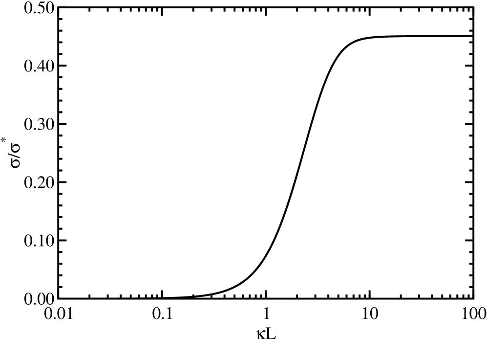
Figure 5: Variation of the surface charge density with $\kappa L$. Note $\sigma^{*}=-\bar{K}_{3}/(2\epsilon)$.

III.3 Casimir Force

We now consider the situation where two, grounded metal plates are immersed in a bulk electrolyte solution. The chemical potentials of the electrolytes in the bulk solution are fixed at $\gamma_{\alpha}=\beta\mu_{\alpha}$, which are identical to the chemical potentials of the electrolytes between the plates. We assume that the thickness of the metal plates is much larger than the size of the electrolytes and much larger than the separation between the plates.

In order to obtain the force between the two plates, we calculate the pressure which is given by

$$p = k_{B}T\frac{\partial\ln Z_{G}}{\partial V}=\frac{k_{B}T}{A}\frac{\partial\ln Z_{G}}{\partial L}$$ (34)

where $A$ is the surface area of the plates, and $V=AL$ is the total volume of the system. We therefore need the full expression for the grand potential $Z_{G}$, which to order one-loop is explicitely obtained from Eq. (II.2) and can be written as (see Appendix B)

$$\ln Z_{G}[\gamma] = AL\sum_{\alpha}\bar{\rho}_{\alpha}-\frac{\kappa^{2}A}{8\pi}I(\kappa L)$$

$$I(\kappa L) \equiv -\frac{2}{(\kappa L)^{2}}\int_{0}^{\kappa L}dxx\ln\left(\frac{\sinh x}{x}\right).$$ (35)

For large values of $L$, the the grand potential behaves as

$$\ln Z_{G}[\gamma] = AL\sum_{\alpha}\bar{\rho}_{\alpha}+AL\frac{\kappa^{3}}{12\pi}-A\left(\ln 2-\frac{1}{2}\right)\frac{\kappa^{2}}{8\pi}$$ (36)

$$\qquad-A\frac{\kappa^{2}}{8\pi}\ln(\kappa L)-\frac{A}{L^{2}}\frac{\zeta(3)}{16\pi}+\cdots$$

where the higher order terms vanish more rapidly than $L^{-2}$ with increasing $L$.

The first two terms are proportional to the volume of the system. This is essentially the Debye-Hückel approximation (order one-loop) for the fluctuation correction for a bulk electrolyte. The third term is proportional to the surface area of the metal plates and is independent of the separation distance $L$. This term is esentially the free energy of creating the metal/electrolyte interfaces. The higher order terms represent the free energy cost of separating the plates. These terms are responsible for inducing a net attraction between the metal plates, as demonstrated next.

Owing to Eqs. (34) and (III.3), the pressure in between the metal plates, due to the presence of the electrolytes, is given by

$$\frac{p(L)}{k_{B}T} = \sum_{\alpha}\bar{\rho}_{\alpha}-\frac{\kappa^{3}}{8\pi}I^{\prime}(\kappa L)$$ (37)

Using the large-$L$ expansion Eq. (36), for $\kappa L\gg 1$ the pressure behaves as

$$\frac{p(L)}{k_{B}T} = \sum_{\alpha}\bar{\rho}_{\alpha}+\frac{\kappa^{3}}{12\pi}-\frac{\kappa^{2}}{8\pi}\frac{1}{L}+\frac{\zeta(3)}{8\pi}\frac{1}{L^{3}}+\cdots$$ (38)

The sum of the first two terms on the right-hand side are equal to the pressure of the bulk solution (i.e., the solution outside the plates). This pressure acts on the outside surface of the plates.

The net attractive force per unit area ${\mathcal{P}}$ acting between the plates is given by the difference in the pressures inside and outside the plates:

$${\mathcal{P}}(L) = p(L,\gamma)-p(\infty,\gamma)$$ (39)

$$= -\frac{k_{B}T\kappa^{3}}{8\pi}\left[I^{\prime}(\kappa L)+\frac{2}{3}\right]$$

In Fig. 6, the variation of this attractive force with plate separation is plotted, while holding the inverse screening length $\kappa$ constant.

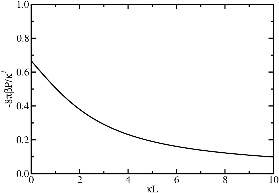
Figure 6: Fluctuation induced attraction between two parallel metal plates separated by a distance $L$.

For small values of $\kappa L$ (e.g., at small plate separations), the force between the plates behaves as

$${\mathcal{P}}(L) \approx -\frac{k_{B}T\kappa^{3}}{12\pi}\left[1-\frac{\kappa L}{4}+\frac{(\kappa L)^{3}}{90}+\cdots\right]$$ (40)

The leading term is proportional to the square root of the temperature. In the limit that the plate separation vanishes, we see the force approaches its maximum value, which is finite.

For large values of $\kappa L$ (e.g., for large plate separations), the force behaves as

$${\mathcal{P}}(L) \approx -\frac{k_{B}T}{8\pi}\frac{\kappa^{2}}{L}\left[1-\frac{\zeta(3)}{(\kappa L)^{2}}+\cdots\right]$$ (41)

The leading order term is independent of temperature. For large plate separations, the force decays inversely with the plate separation.

IV Conclusions

We have performed order one-loop calculations for an electrolyte confined between a pair of grounded, metal plates. For this system, we find that the fluctuation corrections lead to qualitatively different physics than predicted by the mean-field approximation.

The density profiles of the ions are non-uniform. For symmetric electrolytes, the densities of the ions have their minimum values (give by the mean-field values) at the metal interface and are peaked in the center of the system. The magnitude of the density profiles is always lower than the densities of the ions in an equilibrium bulk solution. Despite the non-uniform density distribution, the system still obeys local electrical neutrality, and the electric potential is everywhere zero.

For asymmetric electrolytes, local charge separation can occur. When the plate separation is much less than a screening length, the charge profile has a single peak at the center of the system. When the plate separation becomes much greater than the screening length, the charge profile develops two peaks, with a minimum in the center of the system. This non-uniform charge distribution generates a non-zero electrical potential throughout the system. In addition, a surface charge arises on the metal plates. In the limit of infinite plate separation, this surface charge approaches a finite limit $\sigma/\sigma^{*}\approx 0.451$. In addition, the charge distribution near the plates approaches a limiting form.

When the plates are immersed in a bath of electrolytes, the ion-ion correlations induce an attractive force between them. This force is greatest when the plates are touching and decays as $1/L$ at large plate separation.

In these calculations, the size of the ions was neglected. Consequently, the predictions are valid only in the limit where the plate separations are much greater than the ion sizes. Excluded volume interactions, as well as other types of forces, can be incorporated into the theory by changing the starting partition function Eq. (9) Lue_etal_1999 ; Burak_Andelman_2000 . This method can also be used to study other types of electrolyte systems, such as polyelectrolytes or even quantum systems. This work is currently being pursued.

Appendix A Integrals for density

For the evaluation of the charge density profile in the asymmetric case $\bar{K}_{3}\neq 0$, Eq.(III.1), one requires the following integrals:

$$\int_{0}^{L}dz^{\prime}\Delta G(z^{\prime},z^{\prime})\sin\frac{n\pi z^{\prime}}{L}$$

$$= \frac{1}{\epsilon}\sum_{m=1}^{\infty}\ln\left(1+\left(\frac{\kappa L}{m\pi}\right)^{2}\right)\frac{(2m\pi)^{2}(1-\cos n\pi)}{n\pi[(n\pi)^{2}-(2m\pi)]}$$

and

$$\int d{\bf r}^{\prime}\Delta G({\bf r}^{\prime},{\bf r}^{\prime})G({\bf r}^{\prime},{\bf r})$$

$$= \frac{8\pi}{\epsilon L}\sum_{n=1}^{\infty}\frac{\sin\frac{n\pi z}{L}}{\left(\frac{n\pi}{L}\right)^{2}+\kappa^{2}}\int_{0}^{L}dz^{\prime}\Delta G(z^{\prime},z^{\prime})\sin\frac{n\pi z^{\prime}}{L}$$

$$= \frac{8\pi L}{\epsilon^{2}}\sum_{m=1}^{\infty}(2m\pi)^{2}\ln\left(1+\left(\frac{\kappa L}{m\pi}\right)^{2}\right)$$

$$\qquad\times\sum_{n=1}^{\infty}\frac{(1-\cos n\pi)\sin\frac{n\pi z}{L}}{n\pi[(n\pi)^{2}+(\kappa L)^{2}][(n\pi)^{2}-(2m\pi)]}$$

To perform the summation over the index $n$, we first note the following relation,

$$\sum_{n=1}^{\infty}\frac{n\pi(1-\cos n\pi)\sin\frac{n\pi z}{L}}{(n\pi)^{2}+a^{2}} = \frac{\cosh\frac{a}{2}(2z/L-1)}{2\cosh(a/2)}$$ (44)

which can be verified by expanding the right-side of the expression in a Fourier sine series. In addition, we note that

$$\frac{1}{(n\pi)[(n\pi)^{2}+(\kappa L)^{2}][(n\pi)^{2}-(2m\pi)^{2}]}$$ (45)

$$\quad=\frac{1}{(2m\pi)^{2}+(\kappa L)^{2}}\left\{\frac{1}{(\kappa L)^{2}}\left[\frac{n\pi}{(n\pi)^{2}+(\kappa L)^{2}}-\frac{1}{n\pi}\right]\right.$$

$$\qquad\qquad+\left.\frac{1}{(2m\pi)^{2}}\left[\frac{n\pi}{(n\pi)^{2}-(2m\pi)^{2}}-\frac{1}{n\pi}\right]\right\}.$$

This is used when performing the summation,

$$\int d{\bf r}^{\prime}\Delta G({\bf r}^{\prime},{\bf r}^{\prime})G({\bf r}^{\prime},{\bf r}) = \frac{8\pi L}{\epsilon^{2}}\sum_{m=1}^{\infty}\frac{(2m\pi)^{2}}{(2m\pi)^{2}+(\kappa L)^{2}}\ln\left(1+\left(\frac{\kappa L}{m\pi}\right)^{2}\right)\frac{1}{2}\left\{\frac{1}{(\kappa L)^{2}}\left[\frac{\cosh\frac{\kappa L}{2}(2z/L-1)}{\cosh\frac{\kappa L}{2}}-1\right]\right.$$ (46)

$$\qquad\left.+\frac{1}{(2m\pi)^{2}}\left[\frac{\cos m\pi(2z/L-1)}{\cos m\pi}-1\right]\right\}$$

$$= \frac{4\pi L}{\epsilon^{2}}\frac{1}{(\kappa L)^{2}}\sum_{m=1}^{\infty}\frac{(2m\pi)^{2}}{(2m\pi)^{2}+(\kappa L)^{2}}\ln\left(1+\left(\frac{\kappa L}{m\pi}\right)^{2}\right)$$

$$\qquad\times\left\{\left[\frac{\cosh\frac{\kappa L}{2}(2z/L-1)}{\cosh\frac{\kappa L}{2}}-1\right]+\left(\frac{\kappa L}{2m\pi}\right)^{2}\left(\cos\frac{2m\pi z}{L}-1\right)\right\}$$

$$= \frac{4\pi L}{\epsilon^{2}}\frac{1}{(\kappa L)^{2}}\sum_{m=1}^{\infty}\frac{(2m\pi)^{2}}{(2m\pi)^{2}+(\kappa L)^{2}}\ln\left(1+\left(\frac{\kappa L}{m\pi}\right)^{2}\right)$$

$$\qquad\times\left\{2\frac{\sinh\frac{\kappa L}{2}\frac{z}{L}\sinh\frac{\kappa L}{2}(z/L-1)}{\cosh\frac{\kappa L}{2}}-2\left(\frac{\kappa L}{2m\pi}\right)^{2}\sin^{2}\frac{m\pi z}{L}\right\}$$

$$= \frac{8\pi L}{\epsilon^{2}}\Bigg{\{}\frac{\sinh\frac{\kappa L}{2}\frac{z}{L}\sinh\frac{\kappa L}{2}(z/L-1)}{(\kappa L)^{2}\cosh\frac{\kappa L}{2}}\sum_{m=1}^{\infty}\frac{(2m\pi)^{2}\ln\left(1+\left(\frac{\kappa L}{m\pi}\right)^{2}\right)}{(2m\pi)^{2}+(\kappa L)^{2}}$$

$$\qquad-\sum_{m=1}^{\infty}\frac{\ln\left(1+\left(\frac{\kappa L}{m\pi}\right)^{2}\right)}{(2m\pi)^{2}+(\kappa L)^{2}}\sin^{2}\frac{m\pi z}{L}\Bigg{\}}$$

$$= \frac{8\pi L}{\epsilon^{2}}\left[\frac{\sinh\frac{\kappa z}{2}\sinh\frac{\kappa L}{2}(z/L-1)}{\cosh\frac{\kappa L}{2}}I_{3}(\kappa L)-I_{2}(\kappa L,z)\right]$$

where $I_{2}$ and $I_{3}$ are defined in Eq. (29).

Finally, for the electric potential, we require the derivative

$$\left.\frac{\partial}{\partial z}\int dr^{\prime}\Delta G(r^{\prime},r^{\prime})G(r^{\prime},r)\right|_{z=0}$$ (47)

$$\qquad\qquad=-\frac{4\pi\kappa L}{\epsilon^{2}}\tanh\frac{\kappa L}{2}I_{3}(\kappa L)$$

which can easily be obtained by differentiating Eq. (46).

In order to perform asyptotic analysis for the functions $I_{1}$, $I_{2}$, and $I_{3}$, it is convenient to express them in terms of integrals rather than an infinite series. This can be acheived by first noting that

$$\ln\left(1+\left(\frac{\kappa L}{n\pi}\right)^{2}\right) = \int_{0}^{\kappa L}\frac{2xdx}{(n\pi)^{2}+x^{2}}$$ (48)

and then using the relation:

$$\sum_{n=1}^{\infty}\frac{\cos 2m\pi x}{(2m\pi)^{2}+\alpha^{2}} = \frac{\cosh\frac{\alpha}{2}(1-2x)\alpha}{4\alpha\sinh(\alpha/2)}-\frac{1}{2\alpha^{2}}$$ (49)

It can then be shown that

$$I_{1}(\kappa L,z) = \frac{(\kappa L)}{2}\int_{0}^{2}dx\frac{\sinh\frac{\kappa Lx}{2}(1-z/L)\sinh\frac{\kappa xz}{2}}{\sinh\frac{\kappa Lx}{2}}$$ (50)

$$I_{2}(\kappa L,z) = \frac{1}{2\kappa L}\int_{0}^{2}\frac{xdx}{x^{2}-1}\Bigg{[}\frac{\sinh\frac{\kappa L}{2}(1-z/L)\sinh\frac{\kappa z}{2}}{\sinh\frac{\kappa L}{2}}$$ (51)

$$\qquad-\frac{\sinh\frac{\kappa Lx}{2}(1-z/L)\sinh\frac{\kappa xz}{2}}{x\sinh\frac{\kappa Lx}{2}}\Bigg{]}$$

$$I_{3}(\kappa L) = \frac{1}{2\kappa L}\int_{0}^{2}\frac{xdx}{x^{2}-1}$$ (52)

$$\qquad\times\left(x\coth\frac{\kappa Lx}{2}-\coth\frac{\kappa L}{2}\right)$$

Appendix B One-loop Correction

The one-loop correction to the grand potential is given by the expression

$$\delta\ln Z_{G}[\gamma] = -\frac{1}{2}{\rm Tr}[\ln(1+\bar{K}_{2}G_{0})-\bar{K}_{2}G_{0}]$$ (53)

$$= -\frac{A}{2}\sum_{n=1}^{\infty}\int\frac{dq_{1}}{(2\pi)}\frac{dq_{2}}{(2\pi)}\left\{\ln\left(1+\frac{\kappa^{2}}{(n\pi/L)^{2}+q_{1}^{2}+q_{2}^{2}}\right)-\frac{\kappa^{2}}{(n\pi/L)^{2}+q_{1}^{2}+q_{2}^{2}}\right\}=-\frac{\kappa^{2}A}{8\pi}I(\kappa L).$$

We need to evaluate the following integral

$$I(\kappa L) = \sum_{n=1}^{\infty}\int_{0}^{\infty}dx\left[\ln\left(1+\frac{1}{(n\pi/\kappa L)^{2}+x}\right)\right.$$ (55)

$$\qquad\left.-\frac{1}{(n\pi/\kappa L)^{2}+x}\right]$$

$$= \sum_{n=1}^{\infty}\left\{1-\left[\ln\left(1+\left(\frac{\pi n}{\kappa L}\right)^{2}\right)-\ln\left(\frac{\pi n}{\kappa L}\right)^{2}\right]\right.$$

$$\qquad\left.\times\left[1+\left(\frac{\pi n}{\kappa L}\right)^{2}\right]\right\}.$$

Now, use the relation

$$\int_{0}^{1}dx\ln(1+x/a^{2})=(1+a^{2})\ln(1+1/a^{2})-1$$ (56)

to find

$$I(\kappa L) = -\sum_{n=1}^{\infty}\int_{0}^{1}dx\ln\left(1+\frac{x(\kappa L)^{2}}{\pi^{2}n^{2}}\right)$$ (57)

$$= -\int_{0}^{1}dx\ln\left(\frac{\sinh(\sqrt{x}\kappa L)}{\sqrt{x}\kappa L}\right).$$

$$= -\frac{2}{(\kappa L)^{2}}\int_{0}^{\kappa L}dxx\ln\left(\frac{\sinh x}{x}\right).$$

Asymptotic limits can easily be obtained from this expression. In the limit $\kappa L\to 0$, we find

$$I(\kappa L) = -\frac{2}{(\kappa L)^{2}}\left[\frac{(\kappa L)^{4}}{24}-\frac{(\kappa L)^{4}}{1080}+\cdots\right]$$ (58)

$$= -\frac{(\kappa L)^{2}}{12}+\frac{(\kappa L)^{4}}{540}+\cdots$$

and

$$I^{\prime}(\kappa L) = -\frac{\kappa L}{6}+\frac{(\kappa L)^{3}}{135}+\cdots$$ (59)

On the other hand, in the limit $\kappa L\to\infty$, we find

$$I(\kappa L) = -\frac{2}{3}(\kappa L)+\left(\ln 2-\frac{1}{2}+\ln(\kappa L)\right)$$

$$+ \frac{\zeta(3)}{2}(\kappa L)^{-2}+\cdots$$

and

$$I^{\prime}(\kappa L) = -\frac{2}{3}+\frac{1}{\kappa L}-\frac{\zeta(3)}{(\kappa L)^{3}}+\cdots$$ (61)

References

- (1) G. Gouy, J. Phys. (France) 9, 475 (1910).
- (2) D. L. Chapman, Philos. Mag. 25, 475 (1913).
- (3) J. Israelachvili, Intermolecular and Surface Forces (Academic Press, New York, 1991).
- (4) Y. Levin, Rep. Prog. Phys. 65, 1577 (2002).
- (5) J. Z. Wu, D. Bratko, H. W. Blanch, and J. M. Prausnitz, J. Chem. Phys. 111, 7084 (1999).
- (6) A. G. Moreira and R. R. Netz, Phys. Rev. Lett. 87, 078301 (2001).
- (7) R. Golestanian, M. Kardar, and T. B. Liverpool, Phys. Rev. Lett. 82, 4456 (1999).
- (8) J. Yu, L. Degrève, and M. Lozada-Cassou, Phys. Rev. Lett. 79, 3656 (1997).
- (9) Y. J. Sheng and H. K. Tsao, Phys. Rev. E 66, 040201 (2002).
- (10) D. Henderson and L. Blum, J. Chem. Phys. 69, 5441 (1978).
- (11) R. Kjellander and S. Marcelja, J. Chem. Phys. 82, 2122 (1985).
- (12) P. Attard, D. J. Mitchell, and B. W. Ninham, J. Chem. Phys. 88, 4987 (1988).
- (13) P. Attard, D. J. Mitchell, and B. W. Ninham, J. Chem. Phys. 89, 4358 (1988).
- (14) T. Biben, J.-P. Hansen, and Y. Rosenfeld, Phys. Rev. E 57, R3727 (1998).
- (15) D. Boda, D. Henderson, R. Rowley, and S. Sokolowski, J. Chem. Phys. 111, 9382 (1999).
- (16) D. Boda, W. R. Fawcett, D. Henderson, and S. Sokolowski, J. Chem. Phys. 116, 7170 (2002).
- (17) C. W. Outhwaite, L. B. Bhuiyan, and S. Levine, J. Chem. Soc. Faraday Trans. 2 76, 1388 (1980).
- (18) G. M. Torrie and J. P. Valleau, J. Chem. Phys. 73, 5807 (1980).
- (19) G. Torrie, J. Valleau, and G. Patey, J. Chem. Phys. 76, 4615 (1982).
- (20) A. L. Kholodenko and A. L. Beyerlein, Phys. Rev. A 43, 3309 (1986).
- (21) J. Ortner, Phys. Rev. E 59, 6312 (1999).
- (22) R. R. Netz and H. Orland, Eur. Phys. J. E 1, 203 (2000).
- (23) L. S. Brown and L. G. Yaffe, Phys. Rep. 340, 1 (2001).
- (24) J. D. Jackson, Classical Electrodynamics (Wiley, New York, 1975).
- (25) L. Lue, N. Zoeller, and D. Blankschtein, Langmuir 15, 3726 (1999).
- (26) J. L. Lebowitz and J. K. Percus, J. Math. Phys. 4, 116 (1963).
- (27) R. Podgornik and J. Dobnikar, J. Chem. Phys. 115, 1951 (2001).
- (28) Y. Burak and D. Andelman, Phys. Rev. E 62, 5296 (2000).