Distribution of reflection eigenvalues in many-channel chaotic cavities with absorption

Abstract

The reflection matrix $R=S^{\dagger}S$, with $S$ being the scattering matrix, differs from the unit one, when absorption is finite. Using the random matrix approach, we calculate analytically the distribution function of its eigenvalues in the limit of a large number of propagating modes in the leads attached to a chaotic cavity. The obtained result is independent on the presence of time-reversal symmetry in the system, being valid at finite absorption and arbitrary openness of the system. The particular cases of perfectly and weakly open cavities are considered in detail. An application of our results to the problem of thermal emission from random media is briefly discussed.

Introduction.– When absorption in a cavity is finite, part of the incoming flux gets irreversibly lost in the walls, breaking thus the unitarity of the scattering matrix. The mismatch between incoming and outgoing fluxes in the scattering process can be naturally described by means of the reflection matrix $R=S_{\gamma}^{\dagger}S_{\gamma}$, where $S_{\gamma}$ denotes the subunitary (at nonzero absorption) scattering matrix to be precisely defined below. The matrix $R$ has the positive eigenvalues $r_{c}\leq 1$, the so-called reflection eigenvalues. Their statistical properties in chaotic resonance scattering attract much attention presently, both experimentally Doron et al. (1990); Méndez-Sánchez et al. (2003) and theoretically Bruce and Chalker (1996); Beenakker et al. (1996); Beenakker (1998); Kogan et al. (2000); Ramakrishna and Kumar (2000); Savin and Sommers (2003); Fyodorov (2003), using the random-matrix theory approach Verbaarschot et al. (1985); Beenakker (1997).

In the limit of weak absorption, $R$ was found Doron et al. (1990); Ramakrishna and Kumar (2000) to be related to the Smith’s time-delay matrix at zero absorption those statistical properties were extensively studied in recent time Lehmann et al. (1995a); Fyodorov and Sommers (1997); Savin et al. (2001); Brouwer et al. (1997); Sommers et al. (2001). Such an analysis was recently generalized by us to the case of arbitrary absorption Savin and Sommers (2003), see also Fyodorov (2003) for the related study. In the particular case of the single-channel cavity, obtained results explain partly the recent experiment Méndez-Sánchez et al. (2003) on the reflection coefficient distribution.

The opposite case of a large number of equivalent channels plays an important role in chaotic scattering, corresponding to the semiclassical limit of matrix models Lewenkopf and Weidenmüller (1991); Lehmann et al. (1995b). In this case $N$ strongly overlapping resonances (poles of the $S$-matrix) are excited in the open cavity through the scattering channels, whose number $M$ scales with $N$. A new energy scale appears then in addition to the mean level spacing $\Delta$ of the closed cavity Lehmann et al. (1995b, a): the empty gap between the real axis in the complex energy plane and the cloud of the resonances in its lower half plane. In the physically justified limit $M/N{\ll}1$ Lehmann et al. (1995a) (though both $M,N{\to}\infty$) considered below this gap is given by the well-known Weisskopf width $\Gamma_{W}=MT\Delta/2\pi$, with $T\leq 1$ being the transmission coefficient Lewenkopf and Weidenmüller (1991). In the presence of finite absorption the widths of the resonances acquire an additional contribution, the absorption width $\Gamma_{a}$ Savin and Sommers (2003). The two competing processes, the escape into continuum and dissolution into the walls, are therefore characterized by the ratio $\Gamma_{a}/\Gamma_{W}=\gamma/T$, where the convenient dimensionless parameter $\gamma\equiv 2\pi\Gamma_{a}/\Delta{M}$ measures the absorption strength.

In this paper we derive the probability distribution function $\mathcal{P}(r)=M^{-1}\sum_{c=1}^{M}\overline{\delta(r-r_{c})}$ of reflection eigenvalues, with the bar indicating the statistical average, in the limit of the large number of channels. This function has, in particular, an important application for the statistics of thermal emission from random media and is known only at perfect coupling ($T{=}1$) Beenakker (1998). Here, we calculate it at arbitrary $T$.

Our starting point is the general relation established in Ref. Savin and Sommers (2003) between $R$ and the effective non-Hermitian Hamiltonian $\mathcal{H}=H-(i/2)VV^{\dagger}$ of the open system, with the Hermitian part $H$ standing for the closed counterpart and the amplitudes $V_{n}^{c}$ describing the coupling between $N$ intrinsic and $M$ channel states. It is achieved by making use of the equivalence Kogan et al. (2000); Ramakrishna and Kumar (2000); Savin and Sommers (2003) of uniform absorption to the pure imaginary shift $E_{\gamma}\equiv{E}+\frac{i}{2}\Gamma_{a}$ of the scattering energy $E$, thus giving $S_{\gamma}\equiv{S}(E_{\gamma})=1-iV^{\dagger}(E_{\gamma}-\mathcal{H})^{-1}V$. This leads to the following connection between the reflection matrix $R$ and the time-delay matrix with absorption $Q_{\gamma}$ ($\hbar=1$) Savin and Sommers (2003):

$$R=1-\Gamma_{a}Q_{\gamma}\,,$$ (1)

where $Q_{\gamma}\equiv Q(E_{\gamma})=V^{\dagger}[(E_{\gamma}-\mathcal{H})^{\dagger}]^{-1}(E_{\gamma}-\mathcal{H})^{-1}V$. The distribution function $\mathcal{P}(r)$ is therefore directly related as

$$\mathcal{P}(r)=\gamma^{-1}\mathcal{P}_{\tau}\left(\gamma^{-1}(1-r)\right)$$ (2)

to the distribution $\mathcal{P}_{\tau}(\tau)=M^{-1}\sum_{c=1}^{M}\overline{\delta(\tau-Mq_{c}/t_{H})}$ of the proper delay times (eigenvalues $q_{c}$ of $Q_{\gamma}$) scaled with $M$ and measured in units of the Heisenberg time $t_{H}=2\pi/\Delta$.

The function (2) is normalized to unity. The average reflection coefficient $\langle{r}\rangle=M^{-1}\overline{\mathrm{tr\,}R}$ is given by

$$\langle{r}\rangle=\int_{0}^{1}dr\,r\,\mathcal{P}(r)=\frac{T+\gamma(1-T)}{T+\gamma}\,.$$ (3)

This result follows from the connection Savin and Sommers (2003) between $\langle{r}\rangle$ and the “norm-leakage” decay function $P(t)$ introduced in Savin and Sokolov (1997): $\langle{r}\rangle=1-\gamma[1-\Gamma_{a}\int_{0}^{\infty}dte^{-\Gamma_{a}{t}}P(t)]$. In the limit considered $P(t)$ reduces to the simple exponent $e^{-\Gamma_{W}{t}}$, since the widths ceased to fluctuate Lehmann et al. (1995b); Savin and Sokolov (1997). Below we will also derive Eq. (3) using a different method.

The saddle-point equation.– The scaling limit studied is far from being trivial and can not be obtained from the known expressions for $\mathcal{P}(r)$ at finite $M$ Savin and Sommers (2003) simply by letting $M{\to}\infty$ there. One needs to start from the original definition that determines the seeking distribution through the jump of the resolvent $G(t)=M^{-1}\overline{\mathrm{tr\,}(t-\Gamma_{a}Q_{\gamma})^{-1}}\equiv 1/t+(\gamma/t^{2})K(t)$ along the discontinuity line $t>0$ as follows:

$$\mathcal{P}(r)=\frac{\gamma}{\pi(1-r)^{2}}\mathrm{Im\,}K(t-i0)\big{|}_{t=1-r}\,.$$ (4)

Following Refs. Savin and Sommers (2003); Sommers et al. (2001), one can obtain the exact (at $N{\to}\infty$) representation for $K$, which is convenient for our purposes,

$$K(t)=\left\langle\frac{1}{8}\,\mathrm{str}\left[\left(\Lambda-i\frac{1-t/2}{\sqrt{1-t}}\Lambda_{1}\right)k\hat{\sigma}\right]\right\rangle_{\mathcal{L}}\,,$$ (5)

with the shorthand $\langle(\ldots)\rangle_{\mathcal{L}}=\int\!d\mu(\hat{\sigma})(\ldots)e^{(M/2)\mathcal{L}}$ and

$$\mathcal{L} = (\gamma/t)\,\mathrm{str}[(1-{t/2})\Lambda\hat{\sigma}-i\sqrt{1-t}\Lambda_{1}\hat{\sigma}]$$ (6)

$$-\mathrm{str}\ln[1+(2g)^{-1}(\Lambda\hat{\sigma}+\hat{\sigma}\Lambda)]\,,$$

as the integral over the noncompact saddle-point manifold of the $8{\times}8$ supermatrix $\hat{\sigma}$ subject to the constraint $\hat{\sigma}^{2}=1$. $\Lambda,\Lambda_{1}$ appearing above are the supermatrix analog of the Pauli matrices $\sigma_{3},\sigma_{1}$ and $k=+1(-1)$ in the space of commuting (anticommuting) variables. Definitions of the superalgebra as well as explicit parametrization, which depends on whether TRS is preserved or broken, can be found in Verbaarschot et al. (1985); Efetov (1996). At last, the constant $g=2/T-1\geq 1$ is related to the transmission coefficient $T$.

In the limit $M{\to}\infty$ the integration over $\hat{\sigma}$ can also be done in the saddle-point approximation. Function (5) is given by a saddle-point value of $\hat{\sigma}$, which is found, as usual, by equating the variance $\delta\mathcal{L}$ to zero. The structure of the latter equation is determined by that of $\mathcal{L}$. A careful analysis shows that, independently on TRS, the supermatrix $\hat{\sigma}$ reduces (and so does the corresponding algebra) in the saddle-point to the $2{\times}2$ usual matrix $\sigma=a\sigma_{3}+b\sigma_{1}$ with the imposed constraint $a^{2}+b^{2}=1$. We find that $K=a-ib(1-t/2)/\sqrt{1-t}$, whereas the equation $\delta\mathcal{L}=0$ gives $(\gamma/t)\sqrt{1-t}K+ib/(g+a)=0$. Eliminating in this equation $a$ and $b$, one arrives finally after some algebra at the following saddle-point equation

$$\frac{1}{t}=\frac{1}{2}-\frac{1}{\gamma K}+\frac{(K+g)/2}{\pm\sqrt{(K+g)^{2}+1+4/\gamma^{2}-g^{2}}-2/\gamma}\,,$$ (7)

where the sign “$+$” must be taken. Independently on the taken choice of the sign, equation (7) can be further equivalently represented as the following forth order equation in $K$:

$$\frac{K^{4}+2gK^{3}}{t}(1-\frac{1}{t}) + \frac{K^{2}}{4}\bigl{[}(g+\frac{2}{\gamma})^{2}-\frac{8g}{t\gamma}-(1-\frac{2}{t})^{2}\bigr{]}$$ (8)

$$+ \frac{K}{\gamma}(1-\frac{2}{t})-\frac{1}{\gamma^{2}}=0\,.$$

In the zero absorption limit, $\gamma{\to}0$ with fixed $t/\gamma=\tau$, this equation simplifies to the cubic one found earlier Sommers et al. (2001).

The choice of the sign “$+$” is justified by two reasons. First, only then the complex solution of Eq. (7) yields the distribution $\mathcal{P}(r)$ nonzero at positive $r$. Second, the function $K(t)$, as follows directly from its definition, must have at $t{\to}{-\infty}$ the positive limit $K_{\infty}=t_{H}^{-1}\overline{\textrm{tr\,}Q_{\gamma}}<1$ Savin and Sommers (2003), which is the mean scaled proper delay time $\langle\tau\rangle$. The equation for the latter follows then readily from (8) as $[(g+2/\gamma)^{2}-1]\langle\tau\rangle^{2}+4\langle\tau\rangle/\gamma-4/\gamma^{2}=0$ that gives $\langle\tau\rangle=T/(\gamma+T)$, reproducing thus Eq. (3) by virtue of $\langle{r}\rangle=1-\gamma\langle\tau\rangle$.

The higher moments of the distribution can be easily calculated in the same way, exploiting the $1/t$–expansion further. For example, substituting $K=\langle\tau\rangle+\gamma\langle\tau^{2}\rangle/t+O(t^{-2})$ in (8) and equating there the $1/t$–term to zero, we find $\langle\tau^{2}\rangle=\langle\tau\rangle^{2}[\gamma^{2}+2(\gamma+T)]/(\gamma+T)^{2}$. That yields the variance of reflection eigenvalues as follows:

$$\langle{r^{2}}\rangle-\langle{r}\rangle^{2}=\frac{\gamma^{2}T^{2}(2\gamma+2T(1-\gamma)-T^{2})}{(\gamma+T)^{4}}\,.$$ (9)

Remarkably, the variance and, therefore, fluctuations of $r$ are suppressed in the both limits of weak and strong absorption.

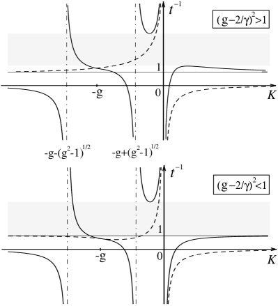
Figure 1: The schematic plot of $1/t$ as a function of $K$. The solid and dashed lines correspond to the choices of “$+$” and “$-$” sign in Eq. (7), respectively. Altogether they form the complete set of solutions of the forth-order equation (8). In the shadowed region the latter equation has two complex-conjugated roots (and two real roots irrelevant for our purposes), with $t^{-1}>1$ ($r>0$). Thus, only in this region the corresponding density is nonzero. Another solution with $0<t^{-1}<1$ is unphysical.

To understand qualitatively the structure of the solutions of the saddle-point equation, it is instructive to consider the behavior of $1/t$ as a function of $K$ shown schematically on Fig. 1. We readily see that the distribution function $\mathcal{P}(r)$ is nonzero only in the finite domain $r_{\mathrm{min}}<r<r_{\mathrm{max}}$. The value of the upper border $r_{\mathrm{max}}<1$ at any $g$ and $\gamma$. In a vicinity of $r_{\mathrm{max}}$ the distribution behaves as $\mathcal{P}(r)\propto\sqrt{r_{\mathrm{max}}-r}$. For the lower border we find $r_{\mathrm{min}}=0$ and $\mathcal{P}(r)\propto 1/\sqrt{r}$, when $(g-2/\gamma)^{2}\leq 1$ or absorption being from the interval $T\leq\gamma\leq T/(1-T)$, and $r_{\mathrm{min}}>0$ with $\mathcal{P}(r)\propto\sqrt{r-r_{\mathrm{min}}}$ otherwise borders . Further analytical study is possible in the following particular cases, which we consider in detail now.

Perfect coupling, $g=T=1$. In this case, the region between the two vertical dash-dotted lines on Fig. 1 shrinks to the line $K=-1$. Eliminating the resulting common factor $(K+1)$, one gets from Eq. (8) the following cubic equation

$$K^{3}+K^{2}+\frac{(1-r)^{2}}{r\gamma^{2}}\Bigl{[}K\bigl{(}\frac{2\gamma}{1-r}-1-\gamma\bigr{)}+1\Bigr{]}=0\,,$$ (10)

written already in the variable $r=1-t$. We find that the discriminant $D=[(1+\gamma)/(3\gamma^{2}r)]^{3}(r_{+}-r)(r-r_{-})(1-r)^{4}$ of this equation, with

$$r_{\pm}=\frac{8+20\gamma^{2}-\gamma^{4}\pm\gamma(8+\gamma^{2})^{3/2}}{8(1+\gamma)^{3}}\,,$$ (11)

is positive at $r>0$ (and thereby $\mathrm{Im}K$ is nonzero) only in the domain $\textrm{max}[0,r_{-}]<r<r_{+}$. This sets explicitly the exact borders for the searched distribution. $\mathcal{P}(r)$ can be found from (10) by applying Cardan’s formulae, reproducing exactly the result of Ref. Beenakker (1998) obtained by a different method. When absorption is weak, $\gamma<1$, the behavior of $\mathcal{P}(r)$ can be well approximated by the following simple interpolation expression interpol :

$$\mathcal{P}_{\gamma<1}(r)=\frac{C_{\gamma}}{2\pi}\frac{\sqrt{(r_{+}-r)(r-r_{-})}}{(1-r)^{2}\sqrt{r}}\,,$$ (12)

with $C_{\gamma}=1+\frac{3}{2}\gamma+O(\gamma^{2})$ being the normalization constant. In the opposite case of strong absorption, the distribution is found to be close to

$$\mathcal{P}_{\gamma>1}(r)=\frac{2\sqrt{1-r_{+}}}{\pi r_{+}}\frac{\sqrt{r_{+}/r-1}}{(1-r)^{2}}\,.$$ (13)

The limiting distribution (12) or (13) becomes asymptotically exact as $\gamma$ diminishes or grows, respectively. All these features are illustrated on Fig. 2a.

Figure 2: The exact reflection distribution (solid lines) compared to the corresponding approximate expressions (12), (13), and (15) at perfect ($T{=}1$, left) and non-perfect ($T{=}0.5$, right) coupling.

Special coupling, $g^{2}=1+4/\gamma^{2}$. Under this condition Eq. (7) reduces to a quadratic equation in $K$, giving readily

$$\mathcal{P}_{g}(r)=\frac{2\sqrt{1-r_{g}}}{\pi r_{g}}\frac{\sqrt{r_{g}/r-1}}{(1-r)^{2}}\,,$$ (14)

with $r_{g}=2/(1+\sqrt{1+\gamma^{2}/4})=2/(1+g/\sqrt{g^{2}-1})$.

Weak coupling, $g\approx 2/T\gg 1$. One can find approximate expressions for $\mathcal{P}(r)$, making use of the scaling $K{\sim}O(1/g)$ in the exact equations. When absorption is weak we may expand the square root in (7) and keep only the main contribution $(2g/\gamma)(1+2gK)^{-1}$ instead of the last term there. That leads again to a quadratic equation in $K$, giving readily the behavior $\mathcal{P}(r)\approx(\gamma/2g\pi^{2})^{1/2}\sqrt{r_{\mathrm{max}}-r}/(1-r)^{2}$ near the upper border $r_{\mathrm{max}}\approx 1-\gamma/8g$. For $\gamma$ from the small interval $[T,T/(1-T)]$, when $r_{\mathrm{min}}{=}0$, $\mathcal{P}(r)$ is given in the leading approximation by Eq. (14), with $r_{g}$ replaced by $r_{\mathrm{max}}$, because the applicability condition for (14) is now satisfied up to $O(g^{-2})$. At other values of small $\gamma$ there is no reliable approximation for the lower border available and $r_{\mathrm{min}}>0$ is to be found from the general equation borders . At last, for very strong absorption and arbitrary non-perfect coupling, $T\neq 1$, we can use scaling $K{\sim}O(1/\sqrt{\gamma})$ in (7). That allows us to replace there the last term with $\frac{1}{2}(K+g)/(1+gK-2/\gamma)$, yielding finally

$$\mathcal{P}_{\gamma\gg 1}(r)=\frac{C}{2\pi}\frac{\sqrt{(r_{0}+\Delta{r}-r)(r-r_{0}+\Delta{r})}}{(1-r)^{2}(1-T+r)}\,,$$ (15)

with the normalization constant $C\approx\gamma-2(1-T)$ and

$$r_{0}\approx 1-T-\frac{2T(2-3T)}{\gamma}\quad\mathrm{and}\quad\Delta{r}\approx 2\sqrt{2}T\sqrt{\frac{1-T}{\gamma}}\,,$$

that is valid when $r_{0}\gg\Delta{r}$ or $\gamma\gg 8T^{2}/(1-T)$. Expression (15) becomes asymptotically exact as $\gamma$ grows, approaching the “semi-circle” distribution with the center at $r_{0}$ and the radius $\Delta{r}$, see Fig. 2b.

Thermal emission.– As an application of our results we consider thermal emission from random media. In his seminal paper Beenakker Beenakker (1998) has shown that the quantum optical problem of the photon statistics can be reduced to a computation of the $S$-matrix of the classical wave equation. In particular, chaotic radiation may be characterized by the effective number $\nu_{\textrm{eff}}$ degrees of freedom as follows: $\nu_{\textrm{eff}}/\nu=(1-\langle{r}\rangle)^{2}/\langle(1-r)^{2}\rangle\leq 1$ Beenakker (1998), with $\nu_{\textrm{eff}}=\nu$ for blackbody radiation Mandel and Wolf (1995). We find using (9) that at any $\gamma$ and $T$

$$\frac{\nu_{\textrm{eff}}}{\nu}=\frac{\langle\tau\rangle^{2}}{\langle\tau^{2}\rangle}=\frac{(\gamma+T)^{2}}{\gamma^{2}+2(\gamma+T)}\,,$$ (16)

and a mean photocount $\bar{n}=\nu f\gamma T/(\gamma+T)$, with $f$ being a Bose-Einstein function. The earlier result Beenakker (1998) is reproduced at $T{=}1$. Upon the substitution of $\gamma$ with $-\gamma$ one can use Beenakker (1998) $\bar{n}$ and $\nu_{\textrm{eff}}/\nu$ (16) even for amplified spontaneous emission below the laser threshold, $\gamma<T$. In this case our mean photocount agrees with the findings of Ref. Hackenbroich et al. (2001), where the general theory of photocount statistics in random amplifying media was developed. In the limit of vanishing absorption or amplification, the ratio $\nu_{\textrm{eff}}/\nu$ is $T/2$. The large $\gamma$ expansion $\nu_{\textrm{eff}}/\nu=1-2(1-T)/\gamma+O(\gamma^{-2})$ shows that the saturation to the blackbody limit gets slower when transmission $T<1$.

In conclusion, for many-channel chaotic systems we have derived the general distribution of reflection eigenvalues at arbitrary values of absorption and transmission. We note that due to a duality relation Beenakker (1998); Paasschens et al. (1996), an amplifying system in the linear regime ($\Gamma_{a}<\Gamma_{W}$) is directly linked to the dual absorbing one through the change of the sign of $\Gamma_{a}$ in (1) and correspondingly thereafter. As a result, the reflection matrices (and their eigenvalues) of dual systems are each other’s reciprocal. Therefore, the analysis presented can straightforwardly be extended to the case of linear amplification that might be also relevant for the rapidly developing field of random lasers Beenakker et al. (1996); Beenakker (1998); Hackenbroich et al. (2001); Paasschens et al. (1996); Cao (2003).

We are grateful to G. Hackenbroich and C. Viviescas for useful discussions. The financial support by the SFB/TR 12 der DFG is acknowledged with thanks.

References

- Doron et al. (1990) E. Doron, U. Smilansky, and A. Frenkel, Phys. Rev. Lett. 65, 3072 (1990).
- Méndez-Sánchez et al. (2003) R. A. Méndez-Sánchez, U. Kuhl, M. Barth, C. H. Lewenkopf, and H.-J. Stöckmann, Phys. Rev. Lett. 91, 174102 (2003).
- Bruce and Chalker (1996) N. A. Bruce and J. T. Chalker, J. Phys. A 29, 3761 (1996);
- Beenakker et al. (1996) C. W. J. Beenakker, J. C. J. Paasschens, and P. W. Brouwer, Phys. Rev. Lett. 76, 1368 (1996).
- Beenakker (1998) C. W. J. Beenakker, Phys. Rev. Lett. 81, 1829 (1998); in Diffusive Waves in Complex Media, NATO ASI Series C531, edited by J.-P. Fouque (Kluwer, Dordrecht, 1999), p.137.
- Kogan et al. (2000) E. Kogan, P. A. Mello, and H. Liqun, Phys. Rev. E 61, R17 (2000).
- Ramakrishna and Kumar (2000) S. A. Ramakrishna and N. Kumar, Phys. Rev. B 61, 3163 (2000). C. W. J. Beenakker and P. W. Brouwer, Physica E 9, 463 (2001).
- Savin and Sommers (2003) D. V. Savin and H.-J. Sommers, Phys. Rev. E 68, 036211 (2003).
- Fyodorov (2003) Y. V. Fyodorov, JETP Lett. 78, 250 (2003); Y. V. Fyodorov and A. Ossipov, cond-mat/0310149.
- Verbaarschot et al. (1985) J. J. M. Verbaarschot, H. A. Weidenmüller, and M. R. Zirnbauer, Phys. Rep. 129, 367 (1985).
- Beenakker (1997) C. W. J. Beenakker, Rev. Mod. Phys. 69, 731 (1997).
- Lehmann et al. (1995a) N. Lehmann, D. V. Savin, V. V. Sokolov, and H.-J. Sommers, Physica D 86, 572 (1995a).
- Fyodorov and Sommers (1997) Y. V. Fyodorov and H.-J. Sommers, J. Math. Phys. 38, 1918 (1997).
- Savin et al. (2001) D. V. Savin, Y. V. Fyodorov, and H.-J. Sommers, Phys. Rev. E 63, 035202(R) (2001).
- Brouwer et al. (1997) P. W. Brouwer, K. M. Frahm, and C. W. J. Beenakker, Phys. Rev. Lett. 78, 4737 (1997); Waves Random Media 9, 91 (1999).
- Sommers et al. (2001) H.-J. Sommers, D. V. Savin, and V. V. Sokolov, Phys. Rev. Lett. 87, 094101 (2001).
- Lewenkopf and Weidenmüller (1991) C. H. Lewenkopf and H. A. Weidenmüller, Ann. Phys. (N.Y.) 212, 53 (1991).
- Lehmann et al. (1995b) N. Lehmann, D. Saher, V. V. Sokolov, and H.-J. Sommers, Nucl. Phys. A 582, 223 (1995b).
- Savin and Sokolov (1997) D. V. Savin and V. V. Sokolov, Phys. Rev. E 56, R4911 (1997).
- Efetov (1996) K. B. Efetov, Supersymmetry in Disorder and Chaos (Cambridge University Press, Cambridge, UK, 1996).
- (21) Equation (8) has two real and one pair of complex conjugated roots only when the corresponding cubic resolvent has also complex roots. Equating the discriminant of the latter to zero yields a forth order equation in , which can be solved, as well as (8), making use of computer algebraic packages. The pair of its real solutions determines thus the borders exactly.
- (22) The square root in the denominator here for close to 1, which could be obtained from a quadratic approximation of Eq. (10) when . It is numerically found that gives the correct tendency at moderate , i.e. an enhancement of at smaller .
- Mandel and Wolf (1995) Registration of photons in the frequency window during the large time yields the negative-bimodal distribution of photocounts with degrees of freedom; see L. Mandel and E. Wolf, Optical Coherence and Quantum Optics (Cambridge University Press, Cambridge, UK, 1995).
- Hackenbroich et al. (2001) G. Hackenbroich, C. Viviescas, B. Elattari, and F. Haake, Phys. Rev. Lett. 86, 5262 (2001).
- Paasschens et al. (1996) J. C. J. Paasschens, T. Sh. Misirpashaev, and C. W. J. Beenakker, Phys. Rev. B 54, 11887 (1996).
- Cao (2003) For a review, see H. Cao, Waves Random Media 13, R1 (2003).