Quantum-to-classical crossover of mesoscopic conductance fluctuations

Abstract

We calculate the system-size-over-wave-length ($M$) dependence of sample-to-sample conductance fluctuations, using the open kicked rotator to model chaotic scattering in a ballistic quantum dot coupled by two $N$-mode point contacts to electron reservoirs. Both a fully quantum mechanical and a semiclassical calculation are presented, and found to be in good agreement. The mean squared conductance fluctuations reach the universal quantum limit of random-matrix-theory for small systems. For large systems they increase $\propto M^{2}$ at fixed mean dwell time $\tau_{D}\propto M/N$. The universal quantum fluctuations dominate over the nonuniversal classical fluctuations if $N<\sqrt{M}$. When expressed as a ratio of time scales, the quantum-to-classical crossover is governed by the ratio of Ehrenfest time and ergodic time.

I Introduction

Sample-to-sample fluctuations of the conductance of disordered systems have a universal regime, in which they are independent of the mean conductance. The requirement for these universal conductance fluctuations Alt85 ; Lee85 is that the sample size should be small compared to the localization length. The mean conductance is then much larger than the conductance quantum $e^{2}/h$.

The same condition applies to the universality of conductance fluctuations in ballistic chaotic quantum dots Bar94 ; Jal94 , although there is no localization in these systems. Random-matrix-theory (RMT) has the universal limit

$$\lim_{N\rightarrow\infty}{\rm var}\,G=\frac{1}{8}$$ (1)

for the variance of the conductance $G$ in units of $e^{2}/h$. Here $N$ is the number of modes transmitted through each of the two ballistic point contacts that connect the quantum dot to electron reservoirs. Since the mean conductance $\left<G\right>=N/2$, the condition for universality remains that the mean conductance should be large compared to the conductance quantum.

In the present paper we will show that there is actually an upper limit on $N$, beyond which RMT breaks down in a quantum dot and the universality of the conductance fluctuations is lost. Since the width $W$ of a point contact should be small compared to the size $L$ of the quantum dot, in order to have chaotic scattering, a trivial requirement is $N\ll M$, where $M$ is the number of transverse modes in a cross-section of the quantum dot. (In two dimensions, $N\simeq W/\lambda_{\rm F}$ and $M\simeq L/\lambda_{\rm F}$, with $\lambda_{\rm F}$ the Fermi wavelength.) By considering the quantum-to-classical crossover, we arrive at the more stringent requirement

$$1\ll N\ll\sqrt{M}e^{\lambda\tau_{\rm erg}/2},$$ (2)

with $\lambda$ the Lyapunov exponent and $\tau_{\rm erg}$ the ergodic time of the classical chaotic dynamics. The requirement is more stringent than $N\ll M$ because, typically, $\lambda^{-1}$ and $\tau_{\rm erg}$ are both equal to the time of flight $\tau_{0}$ across the system, so the exponential factor in Eq. (2) is not far from unity.

Expressed in terms of time scales, the upper limit in Eq. (2) says that $\tau_{\rm erg}$ should be larger than the Ehrenfest time Vav02 ; Sil03

$$\tau_{E}=\max\left[0,\lambda^{-1}\ln\frac{N^{2}}{M}\right].$$ (3)

The condition $\tau_{\rm erg}>\tau_{E}$ which we find for the universality of conductance fluctuations is much more stringent than the condition $\tau_{D}>\tau_{E}$ for the validity of RMT found in other contexts. Lod98 ; Vav02 ; Sil03L ; Jac02 ; Aga00 ; Sil03 ; Two03 ; Ale96 ; Ada03 Here $\tau_{D}\approx(M/N)\tau_{0}$ is the mean dwell time in the quantum dot, which is $\gg\tau_{\rm erg}$ in any chaotic system.

The outline of this paper is as follows. In Sec. II we describe the quantum mechanical model that we use to calculate ${\rm var}\,G$ numerically, which is the same stroboscopic model used in previous investigations of the Ehrenfest time Jac02 ; Two03 ; Gor03 . The data is interpreted semiclassically in Sec. III, leading to the crossover criterion (2). We conclude in Sec. IV.

II Stroboscopic model

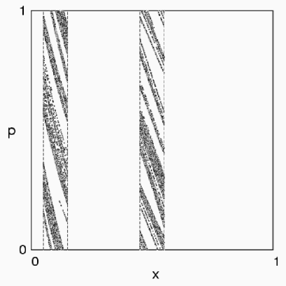
Figure 1: Classical phase space of the open kicked rotator. The dashed lines indicate the two leads (shown for the case $\tau_{D}=5$). Inside each lead we plot the initial and final coordinates of trajectories which are transmitted from the left to the right lead after at most 3 iterations (with $K=7.5$). The points cluster along narrow “transmission bands”.

The physical system we have in mind is a ballistic (clean) quantum dot in a two-dimensional electron gas, connected by two ballistic leads to electron reservoirs. While the phase space of this system is four-dimensional, it can be reduced to two dimensions on a Poincaré surface of section.Bog92 ; Pra03 The open kicked rotator Jac02 ; Two03 ; Gor03 ; Oss02 ; Bor91 ; Bor92 ; Fyo00 is a stroboscopic model with a two-dimensional phase space. We summarize how this model is constructed, following Ref. Two03, .

One starts from the closed system (without the leads). The kicked rotator describes a particle moving along a circle, kicked periodically at time intervals $\tau_{0}$. We set to unity the stroboscopic time $\tau_{0}$ and the Plank constant $\hbar$. The stroboscopic time evolution of a wave function is given by the Floquet operator ${\cal F}$, which can be represented by an $M\times M$ unitary symmetric matrix. The even integer $M$ defines the effective Planck constant $h_{\rm eff}=1/M$. In the discrete coordinate representation ($x_{m}=m/M$, $m=0,1,\ldots,M-1$) the matrix elements of ${\cal F}$ are given by

$${\cal F}_{m^{\prime}m}=M^{-1/2}e^{-i\pi/4}e^{i2\pi MS(x_{m^{\prime}},x_{m})},$$ (4)

where $S$ is the map generating function,

$$S(x^{\prime},x)={\textstyle\frac{1}{2}}(x^{\prime}-x)^{2}-(K/8\pi^{2})(\cos 2\pi x^{\prime}+\cos 2\pi x),$$ (5)

and $K$ is the kicking strength.

The eigenvalues $\exp(-i\varepsilon_{m})$ of ${\cal F}$ define the quasi-energies $\varepsilon_{m}\in(0,2\pi)$. The mean spacing $2\pi/M$ of the quasi-energies plays the role of the mean level spacing $\delta$ in the quantum dot.

To model a pair of $N$-mode ballistic leads, we impose open boundary conditions in a subspace of Hilbert space represented by the indices $m_{n}^{(\alpha)}$. The subscript $n=1,2,\ldots N$ labels the modes and the superscript $\alpha=1,2$ labels the leads. A $2N\times M$ projection matrix $P$ describes the coupling to the ballistic leads. Its elements are

$$P_{nm}=\left\{\begin{array}[]{ll}1&{\rm if}\;\;m=n\in\{m_{n}^{(\alpha)}\},\\ 0&{\rm otherwise}.\end{array}\right.$$ (6)

The mean dwell time is $\tau_{D}=M/2N$ (in units of $\tau_{0}$).

The matrices $P$ and ${\cal F}$ together determine the quasi-energy dependent scattering matrix

$$S(\varepsilon)=P[e^{-i\varepsilon}-{\cal F}(1-P^{\rm T}P)]^{-1}{\cal F}P^{\rm T}.$$ (7)

The symmetry of ${\cal F}$ ensures that $S$ is also symmetric, as it should be in the presence of time-reversal symmetry. By grouping together the $N$ indices belonging to the same lead, the $2N\times 2N$ matrix $S$ can be decomposed into 4 sub-blocks containing the $N\times N$ transmission and reflection matrices,

$$S=\left(\begin{array}[]{cc}r&t\\ t^{\prime}&r^{\prime}\end{array}\right).$$ (8)

The conductance $G$ (in units of $e^{2}/h$) follows from the Landauer formula

$$G={\rm Tr}\,tt^{\dagger}.$$ (9)

The open quantum kicked rotator has a classical limit, described by a map on the torus $\{x,p\;|\;{\rm modulo}\,1\}$. The classical phase space, including the leads, is shown in Fig. 1. The map relates $x,p$ at time $k$ to $x^{\prime},p^{\prime}$ at time $k+1$:

$$p^{\prime}=\frac{\partial}{\partial x^{\prime}}S(x^{\prime},x),\quad p=-\frac{\partial}{\partial x}S(x^{\prime},x).$$ (10)

The classical mechanics becomes fully chaotic for $K\gtrsim 7$, with Lyapunov exponent $\lambda\approx\ln(K/2)$. For smaller $K$ the phase space is mixed, containing both regions of chaotic and of regular motion. We will restrict ourselves to the fully chaotic regime in this paper.

III Numerical results

Figure 2: Variance of the conductance fluctuations obtained numerically by varying $\varepsilon$ with fixed lead positions. Error bars indicate the scatter of values obtained for different lead positions. Results are shown as a function of $1/h_{\rm eff}=M$, for two values of the dwell time $\tau_{D}=M/2N$. The dashed line is the RMT prediction ${\rm var}\,G=\frac{1}{8}$.

To calculate the conductance (9) we need to invert the $M\times M$ matrix between square brackets in Eq. (7). We do this numerically using an iterative procedure. Two03 The iteration can be done efficiently using the fast-Fourier-transform algorithm to calculate the application of $\cal F$ to a vector. The time required to calculate $S$ scales as $M^{2}\ln M$, which for large $M$ is quicker than the $M^{3}$ scaling of a direct inversion. The memory requirements scale as $M$, because we need not store the full scattering matrix to obtain the conductance.

We distinguish two types of mesoscopic fluctuations in the conductance. The first type appears upon varying the quasi-energy $\varepsilon$ for a given scattering matrix $S(\varepsilon)$. Since these fluctuations have no classical analogue (the classical map (10) being $\varepsilon$-independent), we refer to them as quantum fluctuations. The second type appears upon varying the position of the leads, so these involve variation of the scattering matrix at fixed $\varepsilon$. We refer to them as sample-to-sample fluctuations. They have both a quantum mechanical component and a classical analogue. One could introduce a third type of fluctuations, involving both variation of $\varepsilon$ and of the lead positions. We have found (as expected) that these are statistically equivalent to the sample-to-sample fluctuations at fixed $\varepsilon$, so we need not distinguish between fluctuations of type two and three.

Figure 3: Same as Fig. 2, but now for an ensemble in which the lead positions and the quasi-energy are both varied. The dashed lines are the sum of the RMT value (11) and the classical result (12). Results are shown for three values of the kicking strength $K$. Open symbols are for the dwell time $\tau_{D}=10$ and closed ones for $\tau_{D}=20$.

We have calculated the variance ${\rm var}\,G=\left<G^{2}\right>-\left<G\right>^{2}$ of the conductance, either by varying $\varepsilon$ at fixed lead positions (quantum fluctuations) or by varying both $\varepsilon$ and lead positions (sample-to-sample fluctuations). Since the quantum interference pattern is completely different only for energy variations of order of the Thouless energy $1/\tau_{D}$, we choose a number $\tau_{D}$ of equally spaced values of $\varepsilon$ in the interval $(0,2\pi)$. We take $10$ different lead positions, randomly located at the $x$-axis in Fig. 1. To investigate the quantum-to-classical crossover, we change $h_{\rm eff}=1/M$ while keeping the dwell time $\tau_{D}=M/2N$ constant. The results are plotted in Figs. 2 and 3.

IV Interpretation

We interpret the numerical data by assuming that the variance of the conductance is the sum of two contributions: a universal quantum mechanical contribution ${\cal V}_{\rm RMT}$ given by random-matrix theory and a nonuniversal quasiclassical contribution ${\cal V}_{\rm cl}$ determined by sample-to-sample fluctuations in the classical transmission probabilities.

The RMT contribution equals Bar94 ; Jal94

$${\cal V}_{\rm RMT}={\textstyle\frac{1}{8}},$$ (11)

in the presence of time-reversal symmetry. The classical contribution is calculated from the classical map (10), by determining the probability $P_{1\rightarrow 2}$ of a particle injected randomly through lead $1$ to escape via lead $2$. Since the conductance is given semiclassically by $G_{\rm cl}=NP_{1\rightarrow 2}$, we obtain

$${\cal V}_{\rm cl}=N^{2}\,{\rm var}\,P_{1\rightarrow 2}.$$ (12)

We plot ${\rm var}\,G={\cal V}_{\rm RMT}+{\cal V}_{\rm cl}$ in Fig. 3 (dashed curves), for comparison with the results of our full quantum mechanical calculation. The agreement is excellent.

Figure 4: Variance of the classical fluctuations of the transmission probability $P_{1\rightarrow 2}$ upon changes of lead positions, calculated numerically from the map (10). The data is shown for four values of the dwell time $\tau_{D}$, as a function of the Lyapunov exponent $\lambda=\ln(K/2)$. The dotted lines are the analytical prediction (13), with fit parameters $c=1.6$ and $\tau_{\rm erg}=0.68$ (the same for all data sets).

We now would like to investigate what ratio of time scales governs the crossover from quantum to classical fluctuations.

To estimate the magnitude of the sample-to-sample fluctuations in the classical transmission probability, we use results from Ref. Sil03, . There it was found that the starting points (and end points) of transmitted trajectories are not homogeneously distributed in phase space. Instead, they cluster together in nearly parallel, narrow bands. These transmission bands are clearly visible in Fig. 1. The largest band has an area $A_{\rm max}=A_{0}e^{-\lambda\tau_{\rm erg}}$ determined by the ergodic time $\tau_{\rm erg}$. This is the time required for a trajectory to explore the whole accessible phase space. The values of $\tau_{\rm erg}$ and $A_{0}$ depend on the degree of collimation of the beam of trajectories injected into the system. Sil03 For our model, without collimation, one has $\tau_{\rm erg}$ of order unity (one stroboscopic period) and $A_{0}\simeq(N/M)^{2}$. The typical transmission band has an area $A_{0}e^{-\lambda\tau_{D}}$ which is exponentially smaller than $A_{\rm max}$ (since $\tau_{D}=M/2N\gg\tau_{\rm erg}$).

As the position of the lead is moved around, transmission bands move into and out of the lead. The resulting fluctuations in the transmission probability $P_{1\rightarrow 2}$ are dominated by the largest band. Since there is an exponentially large number $e^{\lambda\tau_{D}}$ of typical bands, their fluctuations average out. The total area in phase space of the lead is $A_{\rm lead}=N/M$, so we estimate the mean squared fluctuations in $P_{1\rightarrow 2}$ at

$${\rm var}\,P_{1\rightarrow 2}\simeq(A_{\rm max}/A_{\rm lead})^{2}=c(N/M)^{2}e^{-2\lambda\tau_{\rm erg}},$$ (13)

with $c$ and $\tau_{\rm erg}$ of order unity. We have tested this functional dependence numerically for the map (10), and find a reasonable agreement (see Fig. 4). Both the exponential dependence on $\lambda$ and the quadratic dependence on $\tau_{D}=M/2N$ are consistent with the data. We find $\tau_{\rm erg}=0.68$ of order unity, as expected.

Eqs. (12) and (13) imply

$${\rm var}\,G={\textstyle\frac{1}{8}}+c(N^{4}/M^{2})e^{-2\lambda\tau_{\rm erg}}.$$ (14)

In Fig. 5 we plot the same data as in Fig. 3, but now as a function of $(N^{4}/M^{2})e^{-2\lambda\tau_{\rm erg}}$. We see that the functional dependence (14) is approached for large dwell times.

Figure 5: Same data as in Fig. 3 rescaled to show the approach to a single limiting curve in the large dwell time limit. The solid line is calculated from Eq. (14), with the same parameters $c=1.6$, $\tau_{\rm erg}=0.68$ as in Fig. 4.

The quantum fluctuations of RMT dominate over the classical fluctuations if $N^{2}\,{\rm var}\,P_{1\rightarrow 2}\ll 1$. Using the estimate (13), this amounts to the condition

$$\tau_{\rm erg}>{\rm max}\left[0,\lambda^{-1}\ln(N^{2}/M)\right]\equiv\tau_{E}$$ (15)

that the ergodic time exceeds the Ehrenfest time. Notice that condition (15) is always satisfied if $N^{2}<M\equiv 1/h_{\rm eff}$. This agrees with the findings of Ref. Sil03, , that the breakdown of RMT starts when $N\gtrsim\sqrt{M}$.

V Conclusions

In summary, we have presented both a fully quantum mechanical and a semiclassical calculation of the quantum-to-classical crossover from universal to non-universal conductance fluctuations. The two calculations are in very good agreement, without any adjustable parameter (compare data points with curves in Fig. 3). We have also given an analytical approximation to the numerical data, which allows us to determine the parametric dependence of the crossover.

We have found that universality of the conductance fluctuations requires the ergodic time $\tau_{\rm erg}$ to be larger than the Ehrenfest time $\tau_{E}$. This condition is much more stringent than the condition that the dwell time $\tau_{D}$ should be larger than $\tau_{E}$, found previously for universality of the shot noise in a quantum dot. Aga00 ; Sil03 ; Two03 The universality of the excitation gap in a quantum dot connected to a superconductor is also governed by the ratio $\tau_{D}/\tau_{E}$ rather than $\tau_{\rm erg}/\tau_{E}$ Lod98 ; Vav02 ; Sil03L ; Jac02 , as is the universality of the weak localization effect. Ale96 ; Ada03 These two properties have in common that they represent ensemble averages, rather than sample-to-sample fluctuations.

We propose that what we have found here for the conductance is generic for other transport properties: That the breakdown of RMT with increasing $\tau_{E}$ occurs when $\tau_{E}>\tau_{D}$ for ensemble averages and when $\tau_{E}>\tau_{\rm erg}$ for the fluctuations. This has immediate experimental consequences, because it is much easier to violate the condition $\tau_{E}>\tau_{\rm erg}$ than the condition $\tau_{E}>\tau_{D}$.

To test this proposal, an obvious next step would be to determine the ratio of time scales that govern the breakdown of universality of the fluctuations in the superconducting excitation gap. The numerical data in Refs. Gor03, and Kor03, was interpreted in terms of the ratio $\tau_{E}/\tau_{D}$, but an alternative description in terms of the ratio $\tau_{E}/\tau_{\rm erg}$ was not considered.

One final remark about the distinction between classical and quantum fluctuations, explained in Sec. III. It is possible to suppress the classical fluctuations entirely, by varying only the quasi-energy at fixed lead positions. In that case we would expect the breakdown of universality to be governed by $\tau_{D}/\tau_{E}$ instead of $\tau_{\rm erg}/\tau_{E}$. Our numerical data (Fig. 2) does not show any systematic deviation from RMT, probably because we could not reach sufficiently large systems in our simulation.

Note added: Our final remark above has been criticized by Jacquod and Sukhorukov [Jac03, ]. They argue that the numerical data of Fig. 2 (and similar data of their own) does not show any systematic deviation from RMT because quantum fluctuations remain universal if $\tau_{E}>\tau_{D}$. Their argument relies on the assumption that the effective RMT of Ref. Sil03, holds not only for the classical fluctuations (as we assume here), but also for the quantum fluctuations. The effective RMT says that quantum fluctuations are due to a number $N_{\rm eff}\approx Ne^{-\tau_{E}/\tau_{D}}$ of transmission channels with an RMT distribution. Universality of the quantum fluctuations is then guaranteed even if $N_{\rm eff}\ll N$, as long as $N_{\rm eff}$ is still large compared to unity.

This line of reasoning, if pursued further, contradicts the established theory Ale96 ; Ada03 of the $\tau_{E}$ dependence of weak localization. RMT says that the weak localization correction $\delta G=-\frac{1}{4}$ is independent of the number of channels Bar94 ; Jal94 . Validity of the effective RMT at the quantum level would therefore imply that weak localization remains universal if $\tau_{E}>\tau_{D}$, as long as $Ne^{-\tau_{E}/\tau_{D}}\gg 1$. This contradicts the result $\delta G=\frac{1}{4}e^{-\tau_{E}/\tau_{D}}$ of Refs. Ale96, and Ada03, .

- (1) B. L. Altshuler, JETP Lett. 41, 648 (1985).
- (2) P. A. Lee and A. D. Stone, Phys. Rev. Lett. 55, 1622 (1985).
- (3) H. U. Baranger and P. A. Mello, Phys. Rev. Lett. 73, 142 (1994).
- (4) R. A. Jalabert, J.-L. Pichard, and C. W. J. Beenakker, Europhys. Lett. 27, 255 (1994).
- (5) M. G. Vavilov and A. I. Larkin, Phys. Rev. B 67, 115335 (2003).
- (6) P. G. Silvestrov, M. C. Goorden, and C. W. J. Beenakker, Phys. Rev. B 67, 241301 (2003).
- (7) A. Lodder and Yu. V. Nazarov, Phys. Rev. B 58, 5783 (1998).
- (8) P. G. Silvestrov, M. C. Goorden, and C. W. J. Beenakker, Phys. Rev. Lett. 90, 116801 (2003).
- (9) Ph. Jacquod, H. Schomerus, and C.W.J. Beenakker, Phys. Rev. Lett. 90, 207004 (2003).
- (10) O. Agam, I. Aleiner, and A. Larkin, Phys. Rev. Lett. 85, 3153 (2000).
- (11) J. Tworzydło, A. Tajic, H. Schomerus, and C. W. J. Beenakker, Phys. Rev. B 68, 115313 (2003).
- (12) I. L. Aleiner and A. I. Larkin, Phys. Rev. B 54, 14423 (1996).
- (13) I. Adagideli, Phys. Rev. B 68, 233308 (2003).
- (14) M.C. Goorden, Ph. Jacquod, and C.W.J. Beenakker, Phys. Rev. B 68, 220501 (2003).
- (15) E. B. Bogomolny, Nonlinearity 5, 805 (1992).
- (16) R. E. Prange, Phys. Rev. Lett. 90, 070401 (2003).
- (17) F. Borgonovi, I. Guarneri, and D. L. Shepelyansky, Phys. Rev. A 43, 4517 (1991).
- (18) F. Borgonovi and I. Guarneri, J. Phys. A 25, 3239 (1992).
- (19) Y. V. Fyodorov and H.-J. Sommers, JETP Lett. 72, 422 (2000).
- (20) A. Ossipov, T. Kottos, and T. Geisel, Europhys. Lett. 62, 719 (2003).
- (21) A. Kormanyos, Z. Kaufmann, C. J. Lambert, and J. Cserti, Phys. Rev. B 67, 172506 (2003).
- (22) Ph. Jacquod and E. V. Sukhorukov, cond-mat/0311528.