Reconstruction of the Free Energy in the Metastable Region using the Path Ensemble

Abstract

By quenching into the metastable region of the three-dimensional Ising model, we investigate the paths that the magnetization (energy) takes as a function of time. We accumulate the magnetization (energy) paths into time-dependent distributions from which we reconstruct the free energy as a function of the magnetic field, temperature and system size. From the reconstructed free energy, we obtain the free energy barrier that is associated with the transition from a metastable state to the stable equilibrium state. Although mean-field theory predicts a sharp transition between the metastable and the unstable region where the free energy barrier is zero, the results for the nearest-neighbour Ising model show that the free energy barrier does not go zero.

Keywords: first-order phase transition, nucleation, spinodal, free energy, free energy barrier non-equilibrium statistical physics, Monte Carlo simulation, kinetic Ising model, scaling, mean-field theory, master equation

1 Introduction

Of considerable interest is the calculation of the free energy in the metastable region of a system with a first-order phase transition. The free energy is the starting point for many theories dealing with metastability or spinodal decomposition. The free energy barrier height is needed to calculate the cost of creating a critical droplet formed by statistical fluctuations, which starts the transformation of a metastable state to a stable equilibrium state [1-5]. The calculation of the free energy is therefore central in the development of an understanding of metastability, the spinodal, and the phenomena that arise during a first-order phase transition. It is therefore unfortunate that the free energy cannot be directly measured in a computer simulation [6].

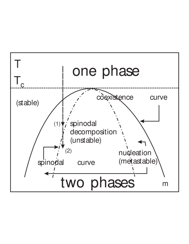
Figure 1: Schematic ($T-m$) phase diagram. Indicated is a temperature quench. Classical theories suggest that relaxation towards equilibrium following a quench in the indicated region (1) proceeds by nucleation and growth. From mean-field theories for the free energy one also obtains a spinodal which separates the metastable region from the unstable

In mean-field theories [5-8] (infinite-range interaction) for the first-order phase transition, one can calculate the free energy not only for the stable equilibrium but also for the non-equilibrium case. It is from this calculation that the distinction is made between metastable and unstable states (see Figure 1). The meta- and unstable states are separated in this framework by a spinodal where the free energy barrier is zero. Within the spinodal region the homogeneous (disordered) phase is thermodynamically unstable. Between the spinodal and the coexistence curve one needs nucleation events of the opposite phase (thermal activation, droplets) to induce the phase transformation.

It has been shown that for systems with short-range interactions, fluctuations will always lead to the decay of a metastable state and drive the system to thermal equilibrium [10, 11]. This does, however, not answer the question of the existence of a spinodal. There have been several attempts to obtain a free energy covering equilibrium and non-equilibrium. Notably Kaski et al. [12] tried to construct the free energy using a coarse-graining procedure. A similar line of reasoning using static concepts is the analytic continuation [13] of the equilibrium free energy into the two-phase region.

Another approach to the problem of nucleation and metastability has been taken by Binder [14]. He considered a single droplet in a finite volume and analysed the corresponding first order phase transition. This, however, does not address the issue whether a spinodal exists and is not able to reconstruct the free energy. It rather assumes a geometric model for the fluctuation and allows comparison to classical theories of nucleation [1, 2]. Here we do not want to make any geometric assumptions for the nucleation events or the functional form of the free energy.

Kolesik et al. [15] can also not reconstruct the spinodal but offer an interesting approach to obtaining the lifetime of metastable states. They look at what they call the projective dynamics [16].

For a quantity such as the energy it is sufficient to take an average over a small representative sample of states, but for the free energy it is necessary to consider all the states accessible to the system. In this work we use the relaxation paths of the system to obtain functionals of the trajectory that the system takes through phase-space [17, 18]. Hence we explore the states accessible to the system escaping a metastable state after a quench. We use the path function to reconstruct the free energy, using the fact that an average of a path function is implicitly an average over a suitably defined ensemble of paths.

We thus start with a description of how we obtain the paths in our Monte Carlo simulation of the three-dimensional Ising model. We use this model because a large body of data is available to facilitate comparision. We discuss the choices for the transition probability which will influence the dynamics of the system and thus the escape from non-equilibrium. We reconstruct the free energy from our simulation data, compare the computed barrier height to mean-field theory and discuss the implications.

2 The Free Energy calculated by paths

The model that we use to study the first-order phase transition is the Ising model. The Hamiltonian of the Ising model for a simple cubic lattice $L^{3}=N$ is defined by

$${\cal H}(s)=-J\sum_{<ij>}s_{i}s_{j}\quad-\mu H\sum_{i}s_{i},\qquad s_{i}=\pm 1$$ (1)

where $J>0$ ($\frac{J}{k_{B}T_{c}}=0.221673$ [19]) is the exchange coupling, $h=2\frac{\mu H}{kT}$ is a dimensionless magnetic field, and $s=(s_{1},s_{2},\ldots,s_{i},\ldots,s_{N})$ denotes a configuration of spins for the lattice. We studied the temperatures $T/T_{c}=0.55$, 0.59, and $0.63$ and fields $h$ ranging from $h=0.4$ to $0.85$.

The above defined Ising model does not have any intrinsic dynamics. It is therefore necessary to construct a Monte Carlo dynamics for the system. The dynamics of the system with respect to Monte Carlo simulations is specified by the transition probabilities of a Markov chain that establishes a path through the available phase space. We have used the Metropolis transition probability [20, 21, 22]

$$W_{M}[s_{i},E_{i}]=\frac{1}{\tau}\min\{1,\exp(-2\beta s_{i}E_{j})\}=W_{M}(s_{i}|s),$$ (2)

where $\beta=1/k_{B}T$ and the Glauber transition probability [20, 21, 22]

$$W_{G}[s_{i},E_{i}]=\frac{1}{\tau}(1-\tanh(\beta s_{i}E_{j})=W_{M}(s_{i}|s).$$ (3)

$\tau$ is a constant setting the time scale. $E_{j}$ denotes the spin and the local field before the spin flip. Here we have excluded the probability for the suggestion of a new state which in our case is a constant. For equilibrium properties it is sufficient that the dynamics satisfies detailed balance so that the correct equilibrium distribution is generated [23]. Starting from an initial configuration $s_{0}$, we get a sequence

$$s^{k}_{0},s^{k}_{1},\ldots s^{k}_{n-1}$$ (4)

of $n$ samples of spin configurations which are dynamically correlated. $k$ denotes the sample of the path. We always start from the same initial condition (all spins down). However, since the random numbers change from run to run, we get a new path for each sample.

Time $t$ in this context is measured in Monte Carlo steps per spin. One Monte Carlo step (MCS) per lattice site, that is, one sweep through the entire lattice, comprises one time unit. Neither magnetization nor energy is conserved in the model, which makes possible to compute energy $e$ and magnetization $m=(1/N)\sum_{i=1}^{N}s_{i}$ as a function of temperature, applied field, time, as well as the system size $N$.

From the point of view of the transition probabilities the dynamic interpretation of the Monte Carlo simulation algorithm stems from the master equation

$$\frac{\partial P(s,t)}{\partial t}=\sum^{N}_{i}W(s|s_{i})P(s_{i},t)-P(s,t)\sum^{N}_{i}W(s_{i}|s),$$ (5)

where the condition of final equilibrium is guaranteed by the above choices of the transition probabilities.

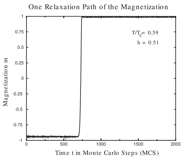
Figure 2: Shown is one example of a relaxation path which is used for the compilation of the probability distribution $P_{N}(m,e,t)$

We now start with a configuration of spins where all spins are $-1$ ($m=-1$) as the initial condition. This corresponds to an equilibrium state of the system. From this state we quench, using the magnetic field $h$ opposite to the magnetization, into the two phase region, that is, to a non-equilibrium magnetization $-m_{coex}(T)\leq m_{meta}\leq m_{coex}(T)$. If $h$ is small enough, the system settles into a metastable state. In Figure 2 we show such a path the magnetization takes from the stable into metastable and then equilibrium state.

Following the magnetization values in time $t$, we get

$$m(t)=(1/N)\sum_{i}s_{i}$$ (6)

for a single quench. For a single quench the values fluctuate after an initial time-lag around a metastable quasi-equilibrium value. After time the magnetization sharply changes its sign and settles into the stable equilibrium value.

The same behaviour is seen for the dimensionless energy per volume as a function of time

$$e(t)=(1/N){\cal H}(s(t)).$$ (7)

Repeating the quench with different initial conditions (here different values for the seed of the random number generator) we obtain a sample of all possible paths from the starting equilibrium state, via the metastable state to the final equilibrium state.

For all the quenches we thus get the time-dependent distribution $P(m,e,N)(t)$ of the magnetization and energy. In Figure 3 we show the evolution of $P(m,N)(t)$ (obtained by ignoring the energy spectrum) for the linear system sizes $L=32$, 64, 128, 265. For $L=32$ the distribution of the magnetization values is rather broad and sharpens considerably with increasing system size. After the initial relaxation the distribution of $P(m,N)(t)$ shows a pronounced peak indicating that the system has spent considerable time in a metastable state. As time progresses, we pick up more contributions from those paths that have already left the average magnetization of the metastable state and are en route to equilibrium.

In equilibrium one can obtain the free energy $F$ of this system by computing the partition function

$$Z=\sum_{s}\exp(-{\cal H}(s)/k_{B}T)$$ (8)

to obtain $F$

$$F=-k_{B}T\ln(Z).$$ (9)

The sum is extended over all possible $2^{N}$ spin configurations.

Here we use the time-dependent distributions for the magnetization and the energy to compute the free energy. We look at the non-equilibrium situation that results after a quench from a stable equilibrium state to a state in the two phase region. The system exhibits a quasi-stable behaviour before it finally reaches stable equilibrium again. We now make use of the dynamics of the system. Starting from equilibrium we perturb the system, applying a magnetic field $h$ opposite to the magnetization $m$, and follow the path the system takes back to equilibrium. Following many such paths we get the path ensemble as defined by the initial thermal equilibrium and the process by which the system is subsequently perturbed from that equilibrium. Distributions and averages are then taken over the ensemble of paths generated by this process.

We define the partition function for each value of the magnetization resulting from the distribution of energy and magnetization by summing over all energy values and over all $t$ in much the same way as was done by [24]

$$Z_{N}(m)=\sum_{e,t=0}^{t_{\max}}P(m,e,N)(t).$$ (10)

Since $t$ is limited in our simulation (the simulation follows the evolution of the spin configurations up to $t_{\max}$) the stable states will be under represented in this summation. These states will contribute to the infinitely deep well of the stable equilibrium state. Then the free energy for each value of magnetization is given by

$$F_{N}(m)=-(k_{b}T)\ln(Z_{N}(m))$$ (11)

or in terms of the exchange coupling $J$

$$F_{N}(m)=-\frac{k_{B}T}{J}\ln(Z(m))\qquad.$$ (12)

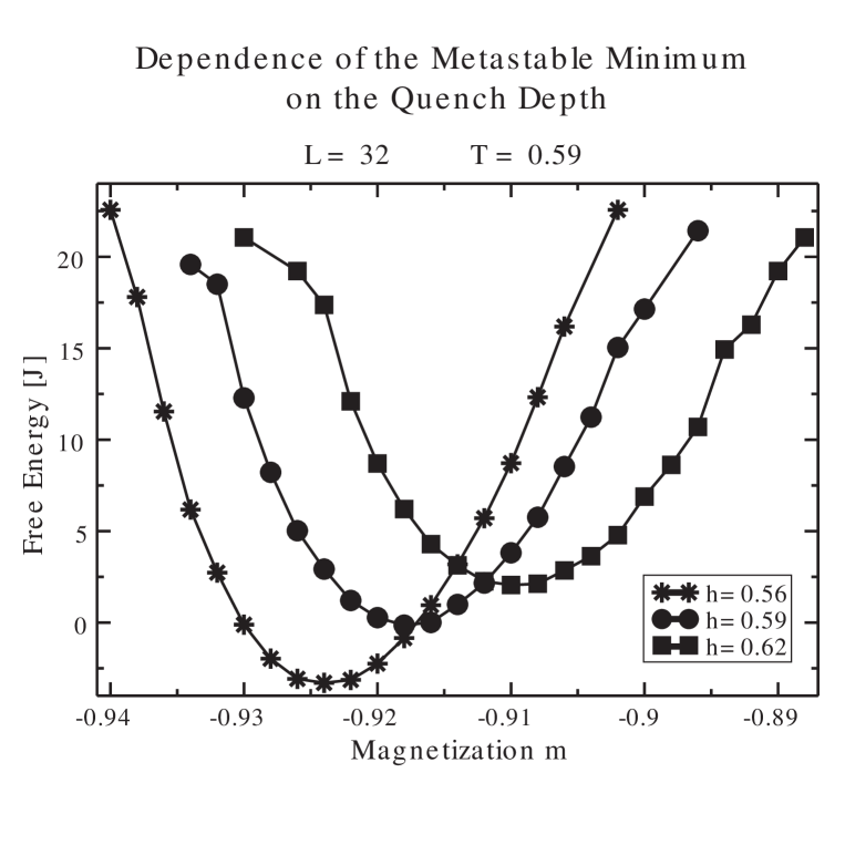
Figure 4: Shown is the free energy minimum which results from a constraint of the summation over time. Here the summation was constrained to include only those times where the magnetization did not drop significantly towards the equilibrium value. Shown are the results for the smallest system size ($L=32$) and three magnetic fields h

If we constrain the summation in Eq. 10 to those times where the system is fluctuating around the metastable magnetization, we would only obtain the metastable minimum of the free energy as shown in Figure 4.

An example of the full dependence of the free energy on $m$ is shown in Figure 5 for one quench depth and temperature. The fact that the minimum of the stable equilibrium state is not infinitely deep is due to the limited summation as discussed above. What is surprising is that the barrier extends over the entire unstable region. Mean field theories suggest a different picture as will be discussed in the next section.

The shift in the metastable minimum as a function of the quench depth is shown in Figure 6. Note that the minimum of the free energy widens considerably as we probe deeper into the metastable/unstable region reflecting the fact that the paths the system takes fluctuate much more than for small $h$. Also the barrier height reduces with increasing $h$.

Most important for the consideration whether there is a clear cut distinction between metastable and unstable states (that is, a spinodal) we have calculated the barrier height in the free energy. The barrier height is defined as the difference between the minimum value of the free energy in the metastable state and the maximum value of the free energy in the unstable part

$$\Delta F_{N}(m)=F_{N}(m_{max})-F_{N}(m_{min}).$$ (13)

We divide out the volume dependence of the free energy and plot in Figure 7 the free energy barrier as a function of the temperature and the applied magnetic field. The barrier height does not go to zero at a finite value of the applied field as suggested by mean-field theories. Rather the barrier height remains finite for those parameters where we still can define a lifetime of a metastable state.

We now take a look at the dependence of the free energy on the transition probabilities. In Figures 8 and 9 we show the free energy for various magnetic fields for the two transition probabilites. While the metastable minimum is not effected by the choice of transition probability, we find the free energy to be shifted in its absolute value. This is to be expected because one can remove the metastable part of the phase diagram altogether for example by using a cluster algorithm [25]. However, the dependence is not very drastic (see below the discussion on the barrier height and its relation to a mean-field spinodal).

3 Comparison to Mean-Field Theories

In mean-field theory for the Ising model we derive the free energy by considering the limit, where all spins interact with each other. In this situation the nearest-neighbour summation in the Hamiltonian factorizes

$${\cal H}(m)=-\frac{1}{2}\frac{T_{c}}{T}m^{2}-hm.$$ (14)

We now consider the entropy of mixing of the states $m$ and $-m$ and find for the free energy the well known result

$$F(h,m)=(\frac{1+m}{2}\ln{\frac{1+m}{2}}+\frac{1-m}{2}\ln{\frac{1-m}{2}})-\frac{1}{2}\frac{T_{c}}{T}m^{2}-hm$$ (15)

for the free energy. A comparison between the predicted mean-field theory and the result from the simulation (c.f. Figure 10) shows clearly that not only the predicted metastable magnetization is wrong, but also the form of the function between the two minima. This holds also for the predicted free energy barrier.

An important theoretical consequence from the above mean-field free energy is the existence of a spinodal [7, 8, 9]. The spinodal is defined to the loci of the points, where the free energy barrier is zero. If there is a spinodal, then we would be able to scale the results of the barrier height as

$$\Delta F=4\left(\frac{T}{T_{c}}\right)(h-h_{\rm sp})^{x}|m_{\rm sp}|^{-1/2}.$$ (16)

In mean-field theory the power of the exponent $x$ is 3/2. However, no consistent set of $h_{\rm sp}$, that is, assuming a spinodal which not necessarily corresponds to the mean-field spinodal, and exponent could be found. Hence, there is not a spinodal in the considered model.

4 Discussion

We have shown that using the ensemble of relaxation paths one can calculate the free energy for finite range interaction models. The kind of analysis presented in this paper very strongly suggests that there is no spinodal, where the free energy barrier is zero, at least for models with short-range potential. We rather find a gradual decrease of the height of the barrier well into the believed unstable part of the two-phase region. It would be interesting to see if one could reconstruct the free energy from the quenches into the unstable region.

5 Acknowledgment

A.T.B and C.E.C would like to thank DAAD and FAPERJ for financial support. We are also very grateful for discussions with D. Stauffer, H. Gould and K. Binder.

Figure 3: Evolution of the distribution of the magnetization at $T/T_{c}=0.59$

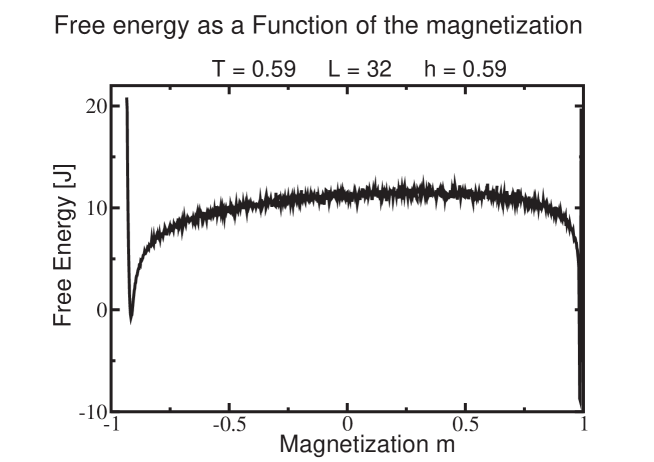
Figure 5: Free energy for a particular quench depth (strength of the magnetic field $h$).

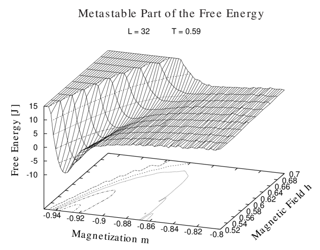
Figure 6: Development of the free energy as a function of the quench depth (strength of the magnetic field $h$)

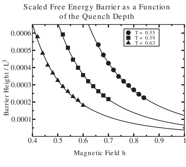
Figure 7: Shown is the free energy barrier height as a function of the quench depth (strength of the magnetic field $h$)

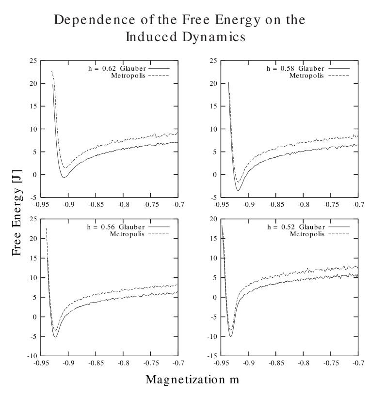
Figure 8: Shown is a comparison of the free energy as a function of the quench depth (strength of the magnetic field $h$) and the induced dynamics by the transition probabilities.

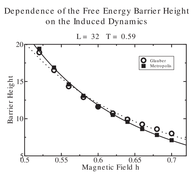
Figure 9: Shown is a comparison of the free energy barrier height as a function of the quench depth (strength of the magnetic field $h$) and the induced dynamics by the transition probabilities.

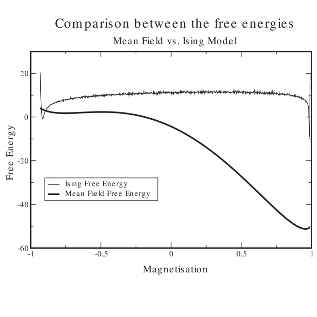
Figure 10: Comparison between the mean-field and the simulation result of the free energy for a particular quench depth (strength of the magnetic field $h$).

References

- [1] R. Becker, W. Döring, Ann. Phys. (Leipzig) 24, 719 (1935)
- [2] A. C. Zettlemoyer (Ed.), Nucleation Theory, Marcel Dekker, New York, 1969
- [3] F.F. Abraham, Homogeneous Nucleation Theory, Academic Press, New York, 1974
- [4] K. Binder and D. Stauffer, Adv. Phys. 25, 343 (1976)
- [5] J. D. Gunton, M. San Miguel, and P. S. Sahini, in C. Domb, J.L. Lebowitz (Eds.), Phase Transtions and Critical Phenomena, Vol. 8, Academic Press, New York (1983)
- [6] C. H. Bennett, J. Comput. Phys. 22, 245 (1976).
- [7] P. A. Rikvold and B. M. Gorma, in D. Stauffer (Ed.), Annual Reviews of Computational Physics I, World Scientific, Singapore, 1994
- [8] K. Binder, in Phase Transformations in Materials, ed. P. Haasen, “Materials Science and Technology”, Vol. 5 VCH Verlag, Weinheim 1991 and S. Komura and H. Furukawa, eds. “Dynamics of Ordering Processes in Condensed Matter”, Plenum Press, New York 1991
- [9] P. A. Rikvold, G. Korniss, C. J. White, M. A. Novotny, and S. W. Sides, in Computer Simulation Studies in Condensed Matter Physics XII edited by D. P. Landau, S. P. Lewis, and H. B. Schüttler, Springer Proceedings in Physics Vol. 85 (Springer, ), 105 (2000)
- [10] G. Sewell Phys. Rep. 57, 307 (1980)
- [11] D. W. Heermann and W. Klein, Phys. Rev. Lett. 50, 1962 (1983).
- [12] K. Kaski, K. Binder, and J. D. Gunton, Phys. Rev. B29, 3996 (1984)
- [13] J. S. Langer, Ann. Phys. N.Y. 54, 258 (1969)
- [14] K. Binder Physica A 319, 99 (2003)
- [15] M. Kolesik, M.A. Novotny and P.A. Rikvold cond-mat/0207405
- [16] M.A. Novotny, M. Kolesik and P.A. Rikvold Comput. Phys. Commun 121-122, 330 (1999)
- [17] W. Paul and D. W. Heermann, Euro.Phys. Lett. 6, 701 (1988)
- [18] W. Paul, D. W. Heermann, and K. Binder J. Phys. A22, 3325 (1989)
- [19] A.L. Talapov and H.W.J. Blöte J. Phys. A: Math Gen. 29, 5727 (1996)
- [20] D. W. Heermann, Computer Simulation Methods in Theoretical Physics 2nd ed., Springer Verlag, Heidelberg, 1990
- [21] K. Binder and D. W. Heermann, “Monte Carlo Simulation in Statistical Physics”, 4-th Edition, Springer, Heidelberg 2002.
- [22] R. J. Glauber, J. Math. Phys. 4, 294 (1963)
- [23] V. I. Manousiouthakis and M. W. Deem, J. Chem. Phys. 110, 2753 (1999).
- [24] I. Shteto, J. Linares, and F. Varret, Phys. Rev. E 56, 5128 (1997)
- [25] D. W. Heermann and A. N. Burkitt, Physica A 162, 210 (1990).