Mean Field Theory of Collective Transport with Phase Slips

Abstract

The driven transport of plastic systems in various disordered backgrounds is studied within mean field theory. Plasticity is modeled using non-convex interparticle potentials that allow for phase slips. This theory most naturally describes sliding charge density waves; other applications include flow of colloidal particles or driven magnetic flux vortices in disordered backgrounds. The phase diagrams exhibit generic phases and phase boundaries, though the shapes of the phase boundaries depend on the shape of the disorder potential. The phases are distinguished by their velocity and coherence: the moving phase generically has finite coherence, while pinned states can be coherent or incoherent. The coherent and incoherent static phases can coexist in parameter space, in contrast with previous results for exactly sinusoidal pinning potentials. Transitions between the moving and static states can also be hysteretic. The depinning transition from the static to sliding states can be determined analytically, while the repinning transition from the moving to the pinned phases is computed by direct simulation.

I Introduction

The collective dynamics of extended systems driven through quenched disorder is a rich and challenging problem, with many experimental realizations. Such systems include vortices in type II superconductors, charge density waves in anisotropic conductors, domain walls in random ferromagnets, and planar cracks in heterogeneous materials.Fisher98 Much of the theoretical work to date has focused on modeling these systems as extended elastic media. In these models the restoring forces are monotonically increasing functions of the relative displacements, and the system is not allowed to tear. At zero temperature, overdamped elastic media subject to an applied force $F$ and quenched disorder exhibit a nonequilibrium phase transition from a pinned state to a sliding state at a critical value, $F_{T}$, of the driving force. DSF85 The depinning transition, first fully studied for collective models with disorder in the context of charge density waves, displays the universal critical behavior of continuous equilibrium phase transitions, with the mean velocity $v$ of the medium playing the role of the order parameter.Fisher98 ; NF92 For monotonic interactions, it has been shown that the system’s velocity is a unique function of the driving force.nocross The sliding state is therefore unique and there is no hysteresis or history dependence. The depinning transition of driven elastic media has been studied extensively, both by functional renormalization group methods NF92 ; Ertas96 ; Wiese02 ; Nattermann and large scale numerical simulations.LittlewoodCoppersmith86 ; LittlewoodCoppersmith87 ; middleton91 ; middleton93 ; MyersSethna93 ; RossoKrauthSimul Universality classes have been identified, which are distinguished, for example, by the range of the interactions or by the periodicity (or nonperiodicity) of the pinning force. More recent work, while still focusing on elastic media, has shown that the dynamics is quite rich well into the uniformly sliding state.koshelev94 ; balents95 ; giamarchi96 ; bmr98 ; moon96 ; pardo98 .

The elastic medium model is often inadequate to describe many real systems which exhibit plasticity (due, for instance, to topological defects in the medium) or inertial effects that violate the assumption of overdamped equations of motion. The dynamics of plastic systems can be both spatially and temporally inhomogeneous, with coexisting pinned and moving regions.coexistnote The depinning transition may become discontinuous (first order), possibly with macroscopic hysteresis and “switching” between pinned and sliding states. Maeda85 ; Maeda90 ; thorne03 ; foot_inertia The theoretical understanding of the dynamics of such “plastic” systems is much less developed than that of driven elastic media. A number of mean-field models of driven extended systems with locally underdamped relaxation or phase slips have been proposed in the literature, Strogatz ; levy92 ; levy94 ; NV97 ; Fisher98 ; MMP00 ; SF01 ; MCMKD02 ; SF03 ; MMSS03 but many open questions remain.

Much of the original theoretical work on driven disordered systems was motived by charge density wave (CDW) transport in anisotropic conductors, which display a nonlinear current-voltage characteristic with a threshold voltage for collective charge transport. gruner ; ThornePhysicsToday It has been known for some time that the elastic depinning transition may not be physically relevant to real CDW materials. coppersmith90 ; SCAM91 ; ThornePhysicsToday Coppersmith argued that in elastic models with weak disorder, unbounded strains can build up at the boundaries of an atypically low pinning region, resulting in large gradients of displacement that lead to the breakdown of the elastic model.coppersmith90 Topological defects or phase slips will occur at the boundaries of such a region, yielding a spatially nonuniform time-averaged velocity. Theoretical and numerical studies of models that incorporate both phase and amplitude fluctuations of the CDW order parameter have indicated that phase slips from large amplitude fluctuations can destroy the critical behavior. balents95 ; myers99 ; karttunen99 The depinning may become discontinuous and hysteretic, or rounded, in the infinite system limit. Experiments show that varying the temperature of the CDW material can lead to a transition from continuous depinning to hysteretic depinning with sharp “switching” between pinned and sliding states.Maeda90 ; switch ; Thorneexpt Furthermore, the observed correlation between the amplitude of broadband noise and macroscopic velocity inhomogeneities also suggest the presence of phase slips.broadband It should be mentioned, however, that in many samples a substantial amount of phase slips occurs at the contacts,lemay98 while less clear evidence exists for substantial phase slip effects in the bulk. In general, CDW experiments display considerable sample-to-sample variability,thorne03 making the comparison between theoretical models and experiments quite challenging.

Related slip effects or plastic behavior have been proposed to explain the complex dynamics of many other dissipative systems, including vortex arrays in type-II superconductors. Simulations (mainly in two dimensions) moon96 ; JensenBrassBerlinskySimul88 ; JensenBrassBrechetBerlinskySimul88 ; NoriSimul96 ; ReichardtOlsonSimul ; GBD ; FMM , imaging pardo98 ; Marchevsky97 ; Troyanovski99 ; STM ; lorenz , and transport and noise experiments fingerprint ; Hellerqvist96 ; maeda02 have shown that driven flux lattices often do not respond as elastic media. Instead, the driven lattice tears as small-scale topological defect structures are generated and healed by the interplay of drive, disorder and interactions. The tearing results in a “plastic” response, with highly defective liquid-like regions flowing around the boundaries of pinned solid-like regions.FMM This kind of response is most prominent in the region near vortex lattice melting, where the so-called peak effect occurs, i.e., the critical current shows a sudden increase with temperature or applied field. Reproducible noise or “fingerprint phenomena” have been observed in the current-dependent differential resistance and attributed to the sequential depinning of various chunks of the vortex lattice.fingerprint Images of driven vortex arrays in irradiated thin films of Niobium obtained by Lorentz microscopy have shown clearly that vortex rivers flowing past each other at the boundaries of pinned regions of the lattice.lorenz Scanning tunneling microscopy, which can resolve individual vortices at high density, has also revealed a clear evolution of the vortex dynamics with disorder strength.Troyanovski99 In samples with weak disorder the vortex array was observed to creep coherently along one of the principal crystal axes near the onset of motion. In samples with strong disorder, the depinning is plastic and the path of individual vortices can be followed as they meander through the pinned crystal. Finally, as in the case of CDWs, a correlation between plasticity and broadband noise has been observed in several samples.maeda02 Recently it has been argued that some of the observed behavior may be due to edge contamination effects that are responsible for the coexistence of a metastable disordered phase and a stable ordered phase. paltiel ; Paltiel02 ; marchevsky It is clear that more work is needed to understand the rich dynamics of these driven systems.

In this paper we study the driven dynamics of a disordered medium with phase slips, in order to better address questions about these and related physical systems. We restrict ourselves to systems which are periodic along the direction of motion, such as CDWs, vortex lattices or 2D colloids, and consider only the dynamics of a scalar displacement field. For concreteness, the model is described in the context of driven CDWs, but it also applies to other driven systems with pinning periodic in the displacement coordinate. Assuming overdamped dynamics and discretizing spatial coordinates, the dynamics of the phase $\theta_{i}$ of each CDW domain is controlled by the competing effects of the external driving force, the periodic pinning from quenched disorder, and the interaction among neighboring domains. Following the literature,Strogatz ; Gorkov ; OngMaki ; inui88 phase slips are introduced by modeling the interactions as a nonlinear sine coupling in the phase difference of neighboring domains. The mean field limit for this type of model has been studied by Strogatz, Westervelt, Marcus and MirolloStrogatz for the case of the smooth sinusoidal pinning force and was shown to exhibit a first order depinning transition, with hysteresis and switching. In this paper we use a combination of analytical methods and numerical simulations to obtain the nonequilibrium mean field phase diagram of the phase slip model for a variety of pinning forces (see Fig. 1). Note that most of the pinning forces we consider are discontinuous. This form of the force mimics the cusped potentials that are the starting points for mean field theories that best reproduce the finite-dimensional results. The discontinuous pinning forces also reflect the abrupt changes in the effective force (sum of elastic and pinning forces) that occur when a neighboring region of the medium suddenly moves forward. We find that discontinuous forces, and even continuous nonsinusoidal pinning forces, yield a rich nonequilibrium phase diagram, with novel stable static phases that are not present for exactly sinusoidal pinning forces.

Figure 1: Sketches of the pinning potentials and forces studied in this paper. The pinning forces are periodic with period $2\pi$ and the pinning potential for a degree of freedom $\theta_{i}$ has minima at $\beta_{i}+2n\pi$, for integer $n$. The cases are organized primarily by the sign of $c$, with the pinning force $Y(x)=-ax-cx^{3}+O(x^{5})$ for small $x=\theta_{i}-\beta_{i}$. The coefficient of the harmonic part of the force satisfies $a>0$. The cases (a), (b) and (c) are for “soft” pinning forces ($c<0$); they differ near the potential maxima, corresponding to monotonic, nonmonotonic, and continuous forces, respectively. Case (d) is a “hard” potential ($c>0$). The “scalloped” potential, case (e), is precisely quadratic ($c=0$) in the interval $-\pi<x<\pi$. The form of the potential especially affects the stability of the coherently pinned phase and whether “reentrant” pinning is possible upon increasing or decreasing the force.

In mean field theory, the nonequilibrium state of the system can be described in terms of two order parameters. As the pinning potential for each domain $i$ is periodic in $\theta_{i}$, having minima at $\beta_{i}+2\pi n$, for integer $n$, and taking the interactions to be periodic in the difference $\theta_{i}-\theta_{j}$ between neighboring phases with the same period, a natural order parameter is the coherence of the phases. This coherence is measured by the amplitude $r$ of a complex order parameter defined via

$$re^{i\psi}=\frac{1}{N}\sum_{j=1}^{N}e^{i\theta_{j}}\;,$$ (1)

with $\psi$ a mean phase. In the absence of interactions among the phases or external drive, the $\theta_{i}$’s are locked to the random phases, $\theta_{i}=\beta_{i}$, and the state is incoherent, with $r=0$. In the opposite limit of very strong interactions we expect perfect coherence of the static state, with all phases becoming equal and $r\to 1$ as the interactions become strong (or the pinning becomes weak.) Another order parameter is the average velocity of the system, given by

$$v=\frac{1}{N}\sum_{j=1}^{N}\dot{\theta}_{j}(t)\;.$$ (2)

The mean velocity is the order parameter for the transition between static and moving phases.

The central results of this paper are the nonequilibrium phase diagrams describing the static and moving phases, for the various pinning forces shown in Fig. 1. The parameters for the phase diagrams are the driving force $F$ and the strength $\mu$ of the interaction between the domains. (For a phase diagram in the drive force vs. pinning strength plane, see Sec.‘VII.) Although the precise shape of the phase boundaries depends on the detailed form of the pinning potential, the types of phases and the schematic topology of the phase diagram are general. This topology and set of phases is exemplified in the phase diagram for the discontinuous soft cubic pinning force (see Fig. 1(b)) shown in Fig. 2. We find three distinct zero-temperature nonequilibrium phases:

• an incoherent static phase (IS) at low drives and small coupling strengths, with $v=0$ and $r=0$;

• a coherent static phase (CS) at low drives and large coupling strengths, with $v=0$ and $r>0$;

• a coherent moving phase (CM) at large drives, with $v>0$ and $r>0$.

We have investigated the possibility of an incoherent moving (IM) phase. For continuous pinning forces, there is no IM phase. For discontinuous pinning forces, we speculate that the IM phase is unstable generically. (See Sec. V where the stability of a possible IM phase is discussed.)

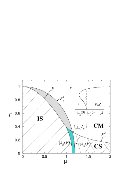
Figure 2: Phase diagram in the coupling-drive ($\mu$-$F$) plane for a discontinuous soft cubic pinning force of the type shown in Fig. 1b. The equation of motion is Eq. (4). The corresponding $Y(x)$ is given by Eq. (34) with $a=15/(8\pi)$ and $c=-4a^{3}/27$. The strength of the pinning is $h=1$ for all degrees of freedom. The diagonally lined region indicates the IS phase, while the cross-hatched region indicates the CS phase. The light gray shaded region denotes the region of coexistence of the CM and IS phases, while the medium gray shaded region denotes the region of coexistence of the IS and CS phases. The lines $F_{\uparrow}^{i}$ and $F_{\uparrow}^{c}$ are the forces at which the system depins upon increasing the drive from the incoherent and coherent static states respectively. The line $F_{\downarrow}$ is the force at which a coherently moving system stops upon lowering the drive. The point $(\mu_{e},F_{e})$ indicates where the static-moving transition goes from hysteretic to non-hysteretic. The curves $\mu_{u}(F)$ and $\mu_{d}(F)$ are the values of the coupling at which the static system makes the transition to and from finite coherence states, respectively. The inset displays the hysteresis in the coherence $r$ as the coupling strength $\mu$ is varied at $F=0$. The transitions between the IS and CS phases are first order in $r$.

An important new feature of the phase diagram is the occurrence of a coherent static phase at finite $F$. In contrast, for the sinusoidal pinning force studied previously by Strogatz and collaborators Strogatz the static state is always incoherent (IS) for all finite values of the driving force and the CS phase is only present at $F=0$.

The location of the transitions between these phases depends on the system’s history. Changing the coupling $\mu$ at fixed drive $F$ can give a hysteretic transition between incoherent and coherent static phases, as shown in the inset of Fig. 2 for $F=0$. Fig. 3 shows the behavior of both the mean velocity and the coherence as $F$ is first increased and then decreased across the boundaries between static and moving phases of Fig. 2, while keeping $\mu$ fixed. The most important features of the phase diagrams are:

• The transition between the IS and CS phases is generally discontinuous. The region of coexistence of coherent and incoherent static states is bounded by curves $\mu_{d}(F)$ and $\mu_{u}(F)$ (or equivalently $F_{d}(\mu)$ and $F_{u}(\mu)$.) When the coupling strength $\mu$ is increased at fixed $F$ within the static region, the system jumps from an incoherent to a coherent state at the critical value $\mu_{u}(F)$, with a discontinuous change in $r$ (see inset of Fig. 2). When $\mu$ is ramped back down, the coherent static state remains stable down to the lower value $\mu_{d}(F)$. The boundaries $\mu_{d}(F)$ and $\mu_{u}(F)$ coincide for the piecewise linear pinning force. In this case the transition is still discontinuous, but not hysteretic. An exception to this general behavior is found for the hard pinning potential at very small values of $F$, where the transition between coherent and incoherent static states is continuous.

• The depinning to the moving phase is discontinuous and hysteretic when the system depins from the IS phase (except when $\mu=0$). When $F$ is increased adiabatically from zero at fixed $\mu$ for a system prepared in the IS phase, both the velocity and the coherence jump discontinuously from zero to a finite value at $F_{\uparrow}^{i}(\mu)$. For an example, see the top frames of Fig. 3. When the force is ramped back down from the sliding state the system gets stuck again at the lower value $F_{\downarrow}(\mu)$.

• The depinning to the moving phase is generally continuous when the system depins from the CS phase. In this case both the velocity and the coherence change continuously at the transition, although they may be non-analytic functions of the control parameters. An example of this behavior is displayed in the bottom frames of Fig. 3. An exception is found for piecewise linear pinning forces (case (e) of Fig. 1) for $\mu\gtrsim\mu_{u}$.

• For continuous pinning forces, the depinning threshold $F_{\uparrow}^{c}(\mu)$ vanishes for $\mu$ above a critical $\mu_{T}$. In contrast, discontinuous pinning forces exhibit a finite depinning threshold for all finite values of $\mu$ with $F_{\uparrow}^{c}(\mu)$ decreasing with increasing $\mu$.

Analytical expressions have been obtained for the critical lines $F^{c}_{\uparrow}(\mu)$ and $F^{i}_{\uparrow}(\mu)$, which give the depinning force values for the coherent and the incoherent static phases, respectively, as well as for the phase boundaries $\mu_{d}(F)$ and $\mu_{u}(F)$, which separate the coherent and incoherent static phases. Numerical simulations of finite mean-field systems have also been used to obtain these boundaries, confirming the analytic stability criteria. The repinning curves ($F_{\downarrow}(\mu)$), where moving solutions stop upon lowering the drive $F$, have been determined numerically.

Figure 3: Typical numerical results, found by integrating numerically the equations of motion (Eq. (4)), for the behavior of the mean velocity $v$ and the coherence $r$ as the driving force is slowly varied. For each pair of plots, the coupling $\mu$ is held constant, while the drive force $F$ is raised from $F=0$ to $F=1.2$ and then decreased. The pinning potential is the same as for Fig. 2. The top frames ($\mu=0.5$) show the hysteretic behavior between the IS and the CM phases, where the coherence and velocity jump between zero and non-zero values at the same locations. The next two sets of frames ($\mu=1.14$) are obtained by preparing the system in the IS-CS coexistence region, starting from either an initial incoherent ($I$) or coherent ($C$) state. When the system is prepared in an incoherent state, the velocity and coherence jump at at the same value of $F$ ($\approx 0.42$) as $F$ is raised, but change continuously as $F$ is decreased, albeit with a change in the slope $dr/dF$ at the repinning force $F\approx 0.32$, where $v$ goes to zero. When the system is prepared in a coherent state, there is no hysteresis and $v$ and $r$ are continuous, though $r$ again shows a singularity at depinning. The bottom frames ($\mu=1.5$) display the behavior at the continuous depinning transition from the CS phase. The results are similar to those for $\mu=1.14$, when starting from the coherent state ($C$). In general, depinning from the coherent state is continuous and non-hysteretic, while depinning from the incoherent state is discontinuous and hysteretic. Numerical evidence for the hysteresis does not change over the size ranges studied, strongly suggesting that these simulations accurately represent the infinite-volume limit.

Part of the motivation for our work comes from the well-known result that the mean field critical exponents for the depinning transition in purely elastic models depend on the details of the pinning force. For instance, the exponent $\beta$ controlling the vanishing of the mean velocity $v$ with driving force at threshold, $v\sim(F-F_{T})^{\beta}$, has a mean field value $\beta=3/2$ for generic smooth continuous pinning forces and $\beta=1$ for a discontinuous piecewise linear pinning force (Fig. 1(e)).AAMthesis Using a functional RG (FRG) expansion in $4-\epsilon$ dimensions, Narayan and Fisher showed NF92 that the discontinuous force captures a crucial intrinsic discontinuity of the large scale, low-frequency dynamics. The FRG calculations give $\beta=1-\epsilon/6+{\cal O}(\epsilon^{2})$, in good agreement with numerical studies in two and three dimensions. The mean field elastic medium also has zero depinning field, $F_{T}=0$, for small pinning strengths $h$, in contrast with finite dimensional simulations and predictions for a finite depinning field in any dimension based on Imry-Ma/Larkin-Ovchinnikov and rare region arguments.DSF85 The RG calculation and the numerics show that a discontinuous pinning force must be used in the mean field theory to incorporate the inherent jerkiness of the motion of finite-dimensional systems at slow velocities. Although there is no reason to believe a priori that the same will hold for models with phase slips, it is clearly important to understand how the properties of the pinning potential affect the nonequilibrium phase diagram of the model. Furthermore, for large coupling strength $\mu$ and bounded pinning force the phase slip model reduces to the elastic model, where the nature of the pinning force strongly affects the mean field theory.

For further applications and connections, we note that models of driven disordered systems with nonmonotonic interactions are also relevant for arrays of nonlinearly coupled oscillators. An example is the Kuramoto model used to describe the onset of synchronization in many biological and chemical systems.kuramoto The model consists of a large number of oscillators with random natural frequencies and a sinusoidal coupling in their local phase differences. Although there is no external drive, this model can exhibit a transition to a synchronized phase as the strength of the coupling is increased. In this phase, all the degrees of freedom oscillate at a common frequency. In the Kuramoto model the natural frequency acts as a random driving force that varies for each oscillator, but there is no random pinning. The model considered here, in contrast, consists of coupled phases, or oscillators, in a random pinning environment at fixed (constant) drive. The onset of coherence (either in a moving or in a static state) corresponds to the onset of the synchronization in the Kuramoto model.

We conclude this introduction by briefly summarizing the remainder of the paper. In Sec. II we describe the model of driven CDWs with phase slips and introduce the mean field limit. In Sec. III we obtain the static solutions of the mean field model at $F=0$ for the selection of pinning forces shown in Fig. 1. We show that the existence of a transition between incoherent and coherent static states can be inferred perturbatively. A full non-perturbative treatment is then applied to understand the nature of the transition. In Sec. IV we consider static states at finite drive. Again, the region of stability of the incoherent static phase can be established by perturbation theory, but the nonperturbative treatment described in Sec. V is needed to map out all the static states and their boundaries of stability to the moving state. The resulting phase diagrams for the various classes of pinning forces are discussed in Sec. V; the analytic calculations supporting these phase diagrams are presented in Appendices A and B. As the analytic treatment we present here is restricted to finding boundaries starting from the static phases, the lower boundary $F_{\downarrow}(\mu)$ of the hysteretic region where static and moving state coexist has been obtained numerically. Sec. VI addresses the effect of a broad distribution of pinning strengths. We conclude in Sec. VII with a discussion of the results and avenues for further studies.

II The model

Though the results of our analysis are more general, we motivate the model with a detailed discussion of the physics of CDWs. The general ideas of phase slip also apply to other systems, most directly to coupled layers of vortices, where the vortices are confined to the planar layers, or to colloidal particles in a disordered background.

A CDW is a coupled periodic modulation of the electronic density and lattice ion positions that exists in certain quasi-one dimensional conductors, due to an instability of the Fermi surface. The undistorted CDW state is a periodic condensate of electrons, characterized by a complex order parameter, with an amplitude $\rho_{1}$ and a phase $\theta$. The electron density can be expanded as $\rho_{e}(x)=\rho_{0}+\rho_{1}\cos[Q_{c}x+\theta(x)]$, with $Q_{c}=2k_{F}$, $k_{F}$ being the Fermi wave vector. The phase $\theta(x)$ describes the position of the CDW with respect to the lattice ions and is a constant for an undistorted CDW. When $Q_{c}$ is incommensurate with the lattice, the CDW can “slide” and CDW transport can be modeled using uniform translations and small gradients of $\theta(x)$, to a first approximation. An applied electric field exceeding a threshold field causes the CDW to slide relative to the lattice at a rate $\partial_{t}\theta$, giving rise to a CDW current. Amplitude fluctuations (changes in $\rho_{1}$) are often neglected because they cost a finite energy, while a vanishingly small energy is required to generate long-wavelength phase excitations, in an ideal crystal. This has led to the well known phase-only model of CDW dynamics introduced by Fukuyama, Lee and Rice (FLR) that incorporates long wavelength elastic distortions of the phase.FLR Strong disorder or regions of unusually low pinning can lead to large strains, however, so that the amplitude can no longer be regarded as constant. Large local strains can be relieved by a transient collapse of the CDW amplitude. One approach to describe such a strongly strained system is a “soft spin” model that considers the coupled dynamics of both phase and amplitude fluctuations. This has been attempted by some authors,balents95 ; myers99 ; karttunen99 but generally leads to models that have to be treated numerically. An alternative, more tractable approach, is to continue to treat the amplitude as constant, while modifying the interaction between phases. This modification should incorporate the crucial feature that the phase becomes undefined at the location where the amplitude collapses. At a strong pinning center, phase distortions can be large and lead to the accumulation of a large polarization that suppresses the CDW amplitude, driving it toward collapse. When the distortion is released through an amplitude collapse, the phase abruptly advances of order $\approx 2\pi$, while the amplitude quickly regenerates.inui88 This process is known as phase slippage in superconductors and superfluids, although it is modified in CDWs because of the physical coupling to the phase. On time scales large compared to those of the microscopic dynamics, it can be described approximately as a “phase slip”: an instantaneous $2\pi$ (modulo $2\pi$) hop of the CDW phase. Following the literature, phase slips will be modeled here as phase couplings periodic in the phase difference between neighboring domains. This leads to a simple model that can be analyzed in some detail.

When modeling CDWs, especially numerically, displacements and amplitudes are coarse-grained to a length scale of order the Imry-Ma-Larkin-Ovchinikov length. At and below this scale, the CDW behaves roughly as a rigid object, referred to as a correlated domain. This domain is taken to move uniformly and is acted upon by driving forces and interactions with neighboring domains and the pinning potential. The continuum space description is replaced with a discrete set of degrees of freedom. The coarse-grained equation of motion for the phase $\theta_{i}$ of a CDW domain $i$ is given by

$${\dot{\theta}_{i}}=F+\mu\sum_{\langle j\rangle}\sin(\theta_{j}-\theta_{i})+h_{i}Y(\theta_{i}-\beta_{i})\;,$$ (3)

where the dot denotes the time derivative (we have chosen to scale time so that the damping constant is unity) and $F$ is the driving force. The second term on the right hand side of Eq. (3) represents the force due to the coupling to other domains, where $\langle j\rangle$ ranges over sites $j$ that are nearest neighbor to $i$ and $\mu$ is the coupling strength. The third term is the pinning force which tends to pin the phase of each domain to a random value $\beta_{i}$ uniformly distributed in $[-\pi,\pi]$. The function $Y(x)$ is periodic with period $2\pi$ and represents the pinning forces. We choose $Y(0)=0$ to fix the location of the minimum of the pinning potential and set $Y^{\prime\prime}(0)=0$ to maintain reflection symmetry in the absence of an external drive. As the potential is minimized at $\theta_{i}=\beta_{i}$, $Y^{\prime}(0)<0$. The random pinning strengths $h_{i}$ are independently chosen from a probability distribution $\rho(h)$.

The key difference between our model equation of motion and the well known FLR elastic model of driven CDWs is in the form of the coupling between domains. Instead of assuming a linear elastic force $\sim\sum_{<j>}(\theta_{j}-\theta_{i})$ between neighboring domains, we have assumed a non-linear, sinusoidal coupling that allows for phase slip processes. For large phase distortions (exceeding $\pi$) the restoring force in Eq. (3) becomes negative and the phases slip by an amount $2\pi$ relative to one another in order to relax the strain.

The starting point for many finite-dimensional theories is the mean field picture where every local phase (or domain) is equally coupled to every other. In this limit, the equation of motion (3) becomes

$${\dot{\theta}}(\beta,h)=F-u\sin(\theta-\psi)+hY(\theta-\beta)\;,$$ (4)

where

$$u\equiv\mu r\;,$$ (5)

measures the effective strength of coupling between the domains and the mean field, with $r$ and $\psi$ defined in Eq. (1). This coupling will only be non-zero if there is some coherence between the phases of different domains, i.e., if $r\neq 0$. For simplicity, we have dropped the subscripts, labeling each phase by the values of $\beta$ and $h$, which are now both continuous variables. The $\beta$ are distributed uniformly in $[-\pi,\pi]$ and the $h$ have the distribution $\rho(h)$.

The self-consistency condition for the mean field theory is given by

$$re^{i\psi}={1\over 2\pi}\int_{-\pi}^{\pi}d\beta\int dh\,\rho(h)e^{i\theta(\beta,h)}\;.$$ (6)

In this paper we will for the most part consider a narrow distribution of pinning strengths, i.e., $\rho(h)=\delta(h-1)$. The effects of a broad distribution $\rho(h)$ will be addressed in Sec. VI.

When the phases are not coupled ($\mu=0$), the equation of motion reduces to that of a single particle, which depins at the single particle threshold force, $F_{\rm sp}$, given by the maximum pinning force. Note that when the coherence $r$ is zero, then $u=0$, and the system may also depin at $F_{\rm sp}$ for a finite value of $\mu$, as long as $r$ remains zero.

III Static States For Zero Drive

We first consider static solutions (${\dot{\theta}}=0$) to Eq. (4) for the case of zero drive ($F=0$). These solutions are the first step in determining the phase diagram and their derivation introduces most of the techniques and concepts used for non-zero drive. When $F=0$, the coherence $r$ is determined by competition between two effects: the disordering effect of the random impurities and the ordering tendency arising from the coupling of each degree of freedom to the mean field. The outcome of this competition gives the $\mu$-dependence of $r$. At zero drive, the system can exist in one of two possible phases: the disordered ($r=0$) IS phase and the ordered ($r>0$) CS phase. These phases can coexist. In this section we examine the nature of the transition between these two phases obtained by varying $\mu$ at $F=0$. We find that the nature of the transition depends on the shape of the pinning force, $Y(x)$.

For static solutions at zero drive, the equation of motion (4) reduces to the condition that the pinning force on each degree of freedom be balanced by the force due to deformations from coupling to the mean field,

$$0=-u\sin(\theta-\psi)+hY(\theta-\beta)\;,$$ (7)

where the reader is reminded that the effective coupling $u$ results from the coupling strength $\mu$ and coherence $r$, $u=\mu r$. For any value of $\mu$ this equation has the trivial solution $\theta=\beta$, $r=u=0$, where all phases rest at the minima of their pinning potentials and the coherence and effective coupling are both zero. It turns out, however, that such a static incoherent solution becomes unstable above a characteristic value of the coupling strength $\mu$.

In order to study the competition between the impurity disordering and mean-field ordering effects, it is useful to rewrite the equation in terms of the deviation $\delta$ of each phase from its value in the disorder dominated incoherent state, $\delta\equiv\theta-\beta$. A direct and important symmetry of the solution of Eq. (7) is global phase invariance, which holds due to the uniform choice of $\beta$. In the static state, this statistical rotational invariance means that we can simply fix $\psi$ to be zero. Given a solution with $\psi=0$, all related solutions with $\psi\not=0$ can then be obtained by letting $\theta\rightarrow\theta+\psi$ and $\beta\rightarrow\beta-\psi$. With this transformations, and specializing to the case of fixed pinning strength, $h=1$, the force balance equation becomes

$$0=-u\sin(\delta+\beta)+Y(\delta)\;.$$ (8)

To solve this force balance equation, we need to determine $u$ self-consistently. The self-consistency condition Eq. (6) can be rewritten, by separating out its real and imaginary parts, as

$$r={1\over 2\pi}\int_{2\pi}d\beta\cos(\delta+\beta)\equiv f(u)\;,$$ (9)

where we have implicitly used Eq. (8) to solve for $\delta$ as a (possibly multi-valued) function of $\beta$ and $u$ to define a function $f(u)$ as the above average over $\beta$, and

$$0=\int_{2\pi}d\beta\sin(\delta+\beta)\;.$$ (10)

Next, we will use a straightforward linear stability analysis to show that the IS ($r=0$) phase becomes unstable to the CS ($r>0$) phase above a critical value $\mu_{u}$ of the coupling strength. A perturbative calculation of $r(\mu)$ allows us to establish that this transition from the IS to the CS phase is continuous or hysteretic, depending on the shape of the pinning potential near its minimum. We will then obtain the full solution $r(\mu,F=0)$ for a variety of pinning forces.

III.1 Stability of the Incoherent Static Phase

To investigate the linear stability of the IS phase, we calculate the time evolution of a configuration near the static solution $\delta(\beta)=0$. A convenient perturbed configuration is $\delta(\beta,t=0)=-\epsilon(0)\sin\beta$ with $\epsilon(0)\ll 1$. This perturbation gives non-zero coherence while maintaining $\psi=0$ and reflects the most rapidly growing eigenvector in the stability analysis, with $\delta(\beta,t)=-\epsilon(t)\sin\beta$ to lowest order in $\epsilon$. By Eq. (9), the coherence of the perturbed state is

$$r = {1\over 2\pi}\int_{-\pi}^{\pi}d\beta\cos(\beta-\epsilon\sin\beta)\;,$$ (11)

$$= \epsilon/2+O(\epsilon^{2})\;.$$

The equations of motion Eq. (4) then give

$${\dot{\delta}} = -\mu r\sin(\beta+\delta)+hY(\delta)$$ (12)

$$= -\mu(\epsilon/2)\sin\beta+hY^{\prime}(0)\delta+O(\epsilon^{2})$$

$$= \left(\frac{\mu}{2}+hY^{\prime}(0)\right)\delta+O(\epsilon^{2})\;.$$

As $r$ and $\delta$ are both proportional to $\epsilon$ (to lowest order), it immediately follows that ${\dot{r}}\approx\left({\mu\over 2}+hY^{\prime}(0)\right)r$. The critical value of $\mu$ for linear stability is therefore

$$\mu_{u}=-2hY^{\prime}(0)\;.$$ (13)

For coupling strength $\mu>\mu_{u}$, the perturbed coherence grows and the IS phase is linearly unstable to a CS phase. At larger $\mu$, the interactions that drive the $\theta$ towards a coherent state are larger in magnitude than the restoring force for the individual $\theta$. Note that $\mu_{u}$ depends only on the strength of the pinning force at the minimum of the pinning potential.

III.2 Perturbation Theory

The onset of coherence for $\mu$ just above $\mu_{u}$ can be studied perturbatively by assuming that both the phase $\delta$ and the coherence $r$ are small in this region. Near $\delta=0$ the pinning force can quite generally be written as a power series in $\delta$,

$$Y(\delta)=-a\delta-b\delta^{2}-c\delta^{3}+...\;,$$ (14)

with $a=-Y^{\prime}(0)>0$. For small $r$, and hence $u$, one can expand $\delta(\beta,u)$ in powers of $u$,

$$\delta(\beta,u)=u\delta_{1}(\beta)+u^{2}\delta_{2}(\beta)+u^{3}\delta_{3}(\beta)+...\;.$$ (15)

Substituting these terms into the force balance equation Eq. (8), and equating terms of the same order in $u$, we obtain

$$\delta_{1}(\beta) = -{\sin\beta\over a}\;,$$ (16a)

$$\delta_{2}(\beta) = {\sin\beta\cos(\beta)\over a^{2}}-{b\sin^{2}\beta\over a^{3}}\;,$$ (16b)

$$\delta_{3}(\beta) = \left({c\over a^{4}}+{2b^{2}\over a^{5}}-{1\over 2a^{3}}\right)\sin^{3}\beta$$ (16c)

$$- {\sin\beta\cos^{2}\beta\over a^{3}}+{3b\sin^{2}\beta\cos\beta\over a^{4}}\;.$$

Substituting the expanded $\delta(\beta,u)$ into Eq. (9) and evaluating the integrals to each order in $u$ we find

$$f(u)=ur_{1}+u^{2}r_{2}+u^{3}r_{3}+\dots\;,$$ (17)

with

$$r_{1} = {1\over 2a}\;,$$ (18a)

$$r_{2} = 0\;,$$ (18b)

$$r_{3} = -{3\over 8}\left({ac-2b^{2}\over a^{5}}\right)\;.$$ (18c)

Finally, the coherence $r$ is given by the solution of

$$r=f(r\mu)=(r\mu)r_{1}+(r\mu)^{3}r_{3}+\dots\;.$$ (19)

For simplicity of discussion we specialize to pinning potentials with reflection symmetry and choose $b=0$ (although the non-zero $b$ result will prove useful in the analogous finite $F$ perturbation theory). Then $r_{3}=-3c/(8a^{4})$ and the nonvanishing solution for the coherence can be written as

$$r(\mu)=\begin{cases}\left(\frac{\mu_{u}^{4}}{3|c|\mu^{3}}\right)^{1/2}\left({\mu_{u}-\mu\over\mu_{u}}\right)^{1/2}&c<0,\\ \left(\frac{\mu_{u}^{4}}{3c\mu^{3}}\right)^{1/2}\left({\mu-\mu_{u}\over\mu_{u}}\right)^{1/2}&c>0,\end{cases}$$ (20)

where $\mu_{u}=2a$.

The behavior of $r(\mu)$ for $\mu\approx\mu_{u}$ and the nature of the transition between the IS and CS phases are controlled by the sign of the coefficient $c$ of the cubic term of $Y(\delta)$. The three types of behavior that can occur are shown in Fig. 4. For $c>0$, corresponding to a “hard” pinning potential that grows more steeply than a parabola near its minimum, the coherence $r$ grows monotonically with increasing $\mu$, with $r\sim(\mu-\mu_{u})^{1/2}$. This indicates a continuous transition at $\mu=\mu_{u}$ between the IS and CS phases. On the other hand, when $c<0$, corresponding to a “soft” pinning potential, the coherence starts out with a negative slope at $\mu_{u}$ and grows with decreasing $\mu$. We expect this solution to be unstable, indicating that the transition from the IS phase to the CS phase occurs with a discontinuous jump in $r$ from $r=0$ for $\mu<\mu_{u}$ to a non-zero value of $r$ for $\mu>\mu_{u}$ on a stable upper branch not accessible in perturbation theory. In fact we show below that when $\mu$ is decreased back down through $\mu_{u}$ from the CS phase $r$ will remain non-zero down to a lower value $\mu_{d}<\mu_{u}$, indicating a hysteretic transition between the IS and CS phases. In the marginal case of piecewise linear pinning forces with $c=0$, i.e., $Y(\delta)=-a\delta$ near $\delta=0$, there is a discontinuous jump $r(\mu)$ at $\mu=\mu_{u}$. In this case the perturbation theory breaks down and the solution must be obtained by the method described in Sec. III.3. This calculation will show that no hysteresis occurs in the case of strictly linear pinning force. We stress that the transition from the IS to the CS state at $F=0$ is controlled entirely by the shape of the pinning potential near its minimum. Specifically, the behavior is unaffected by the existence of discontinuities in the pinning force at the edges of each pinning well.

Figure 4: The behavior of the coherence $r$ for couplings $\mu\approx\mu_{u}$, i.e., near the instability point of the incoherent static phase (IS) at $F=0$. The three curves show $r$ with pinning force $Y(\delta\ll 1)=-a\delta-c\delta^{3}$ for $c$ positive (hard pinning potential), negative (soft pinning potential) and zero (piecewise linear pinning force.)

III.3 Beyond Perturbation Theory: The General Static ${\bf r(\mu,F=0)}$ Solution

In this section we outline a non-perturbative method for calculating the integral $f(u)$ used in the self-consistency equation, Eq. (9). This allows for the determination of the coherence $r$ for all values of $\mu$. In addition to confirming the perturbative results obtained above, this method allows the precise study of the discontinuous and hysteretic transitions between the IS and CS phase, which cannot be done within perturbation theory.

To obtain $f(u)$ by direct integration over $\beta$ in Eq. (9) one would need to solve the transcendental equation, Eq. (8), for $\delta(\beta,u)$. Such a solution cannot in general be obtained analytically. Hence we take an alternative approach in which we solve Eq. (8) for $\beta(\delta,u)$ and integrate over $\delta$, rather than $\beta$, i.e.,

$$r={1\over 2\pi}\int d\delta\left({\partial\beta\over\partial\delta}\right)\cos(\delta+\beta(\delta,u))\;.$$ (21)

The change of variable in Eq. (21) provides an important simplification that allows us to calculate analytically the coherence of the undriven static state for a general pinning potential. This simplification does rely on understanding the subtleties of how $\delta$ depends on $\beta$, as $\delta$ can be multivalued function of $\beta$. The history of the sample can determine which branch(es) are included in the configuration.

For a given $u$, there is an infinite set of solutions to Eq. (8). We index each with an integer $n$:

$$\beta_{n}(\delta,u)=-\delta+n\pi+(-1)^{n}\sin^{-1}(Y(\delta)/u)\;,$$ (22)

where we choose the $[-\pi/2,\pi/2]$ branch for $\sin^{-1}(x)$. The range for $\delta$ is constrained to $-\delta_{\max}(u)\leq\delta\leq\delta_{\max}(u)$, with $\delta_{\max}(u)\equiv Y^{-1}(u)$.

The calculation of the average in Eq. (21) is easily carried out when $u<a$, where the phase is single valued. For values of $u>a$ the function $\delta(\beta)$ is multivalued, allowing for the existence of many metastable static configurations at fixed $u$. Figure (5) shows one such multivalued $\delta(\beta)$. Because of the metastability, the coherence can vary over some range. For a fixed $u$, the range in coherence results in a range of couplings $\mu$. When $u\geq a$ and $\delta(\beta)$ is multivalued, one chooses the (stable) branch of the $\beta(\delta)$ curve that is consistent with the particular metastable state one wishes to describe and also ensures that $\psi=0$, or equivalently that Eq. (10) is satisfied. For simplicity and correspondence with “typical” sample preparation, we focus on those metastable states accessed by adiabatically increasing $u$ from zero.adiabatic_u_footnote These correspond, for a given $u$, to the solid portions of the curve shown in Fig. (5). The details of the calculation for the scenario of adiabatically increasing $u$, which selects one branch, are given in Appendix A. It is relatively straightforward to show that for a given $u$ these are the states which have the largest coherence. This selection of largest-$u$ states is consistent with our numerical calculations. Note that the form of the $\delta(\beta)$ curve and the discussion of multiple solutions is formally quite similar to parts of the calculation for the purely elastic case, though the physical motivation is rather different.DSF85

Figure 5: A sample plot of $\delta$, the displacement of a degree of freedom from the minimum of the pinning potential, versus the pinning phase $\beta_{n}(\delta)$ for branch numbers $-2\leq n\leq 2$. The solid portions correspond to even $n$, while the dashed portions correspond to odd $n$. The global phase $\psi$ is chosen to be zero. Here, the effective interaction is large enough, $u>a$, that $\delta(\beta)$ is multivalued. The maximum magnitude of $\delta$ is denoted by $\delta_{\max}$.

The behavior of the coherence as a function of $\mu$ is shown in Fig. 6 for four pinning potentials (for histories where the effective coupling $u$ is adiabatically increased.) As anticipated on the basis of the perturbation theory, for a hard pinning force (curve (a) of Fig. 6) the coherence is a single-valued function of $\mu$. The system exists in the zero-$r$ IS phase for $\mu<\mu_{u}$. At $\mu_{u}$ there is a continuous transition to the CS phase, with $r$ growing continuously from zero. For soft pinning forces (curves (c), cubic pinning force, and (d), sine pinning force, of Fig. 6) with $c<0$ the coherence is a multivalued function of $\mu$. In this case the IS phase is stable up to $\mu_{u}$ when $\mu$ is ramped up from below. At $\mu_{u}$ the coherence jumps discontinuously to the stable upper branch of the curve corresponding to the CS phase. When $\mu$ is ramped down from above $\mu_{u}$, the system remains in the CS phase down to the lower value $\mu_{d}$. For this class of pinning forces, the IS-CS transition is always hysteretic at $F=0$. In the marginal case of a piecewise linear pinning force (curve (b)), $r$ jumps discontinuously at the transition, but there is no hysteresis.

Figure 6: The coherence of the static state at $F=0$ as a function of the coupling strength $\mu$ for four pinning forces: (a) hard ($c>0$) cubic pinning force, with $a=c=1/(\pi+\pi^{3})$; (b) piecewise linear pinning force, with $a=1/\pi$; (c) soft ($c<0$) cubic pinning force, with $a=1/\pi$ and $c=-1/\pi^{3}$; (d) sine pinning force whose maximum strength is $1/\pi$. Also shown is the value $\mu_{d}$ where the coherence jumps from a finite value to zero upon decreasing $\mu$.

The coherence curves shown in Fig. 6 correspond to the metastable states that would result through adiabatically increasing $u$. As mentioned earlier, for a given $u$, this is the state whose phases are as close as possible to the global phase $\psi=0$, and hence is the state with the largest coherence. Thus, the curves shown in Fig. 6 are upper bounds on the coherence for each type of pinning force. In order to calculate the lowest possible coherence at each $u$, one must consider the metastable state whose phases are as far as possible from the global phase. To obtain this lower $r(\mu)$ bound analytically is tedious, and we have done so only for the sawtooth linear case. This result for the lower bound is displayed in Fig. 7, along with the upper bound, which, again, is the relevant state for the histories we consider here.

Figure 7: Upper and lower bounds for $r(u)$, plotted as the coherence $r(\mu=u/r)$, corresponding to the maximal and minimal coherence static metastable states. The pinning force is taken to be piecewise linear with $a={1/\pi}$. A single static coherent solution is obtained only in the limit $\mu\rightarrow\infty$.

In addition to determining the transitions between the IS and CS phases, the non-perturbative treatment at zero drive can also be used to determine if there is a critical value of $\mu$, $\mu_{T}$, above which the depinning threshold vanishes and the system is always sliding for all $F>0$. We present an outline of the argument here and relegate the details of the calculation of $\mu_{T}$ to Appendix A. The threshold force can be thought of as the largest value of the driving force at which there still exists a stable static solution to the equation of motion. All such solutions satisfy the static self-consistency condition. For incoherent static solutions, in which the domains are completely decoupled, this threshold force is simply the single particle depinning force. For coherent static states the solution $\delta(\beta)$ is multivalued, but only those metastable states which satisfy the imaginary part of the self-consistency condition are acceptable solutions. Consider a system in which there are multiple metastable static solutions at zero drive. When an infinitesimal driving force is applied a correspondingly infinitesimal number of these states becomes unstable as they no longer satisfy the self-consistency condition. The system remains, however, pinned provided there still exist other accessible static metastable states. As the force is further increased, more static states become unstable, but the system does not depin until the “last” of the available static solutions, that is the one corresponding to the largest value of $F$ for which a metastable static state exist, becomes unstable. This value of $F$ defines the depinning threshold. On the other hand, if there is a unique metastable static solution at zero drive, the system will depin immediately upon an infinitesimal increase of the driving force. Whenever there is a unique solution at $F=0$, the depinning force is therefore zero. As shown in Appendix B, for discontinuous forces there are always a variety of metastable static states at zero drive for any finite value of $\mu$ (see also Fig. 7), so that $\mu_{T}=\infty$. For continuous pinning forces, there is a finite coupling $\mu_{T}$ above which there is a single static state at zero drive and where the threshold force vanishes. This is for instance the case for the sinusoidal pinning force, where the upper and lower bounds of $r(\mu)$ (shown in Fig. 6) coincide and $\mu_{T}=\mu_{u}$. For a general continuous pinning force $\mu_{T}$ is given by

$$\mu_{T}={\pi|Y^{\prime}(\pi)|\over\int_{0}^{\pi}d\delta\sqrt{1-(Y(\delta)/Y^{\prime}(\pi))^{2}}}\;.$$ (23)

IV Stability of the Static Incoherent Phase at Nonzero Drive

We next consider static states in the presence of a finite driving force, $F\neq 0$, starting with incoherent static solutions. We will use a perturbative treatment analogous to that of Sec. III to analyze the limit of stability of the IS phase against varying $\mu$ and $F$. For finite $F$, the IS phase can become unstable to either the coherent static phase or the moving phase. The perturbative analysis described in this section allows us to establish whether the transition from the IS to CS phase at finite $F$ is continuous or hysteretic, in much the same way as done in Sec. III.2 for $F=0$. Again we find that the nature of the transition depends on the type of pinning potential, but the addition of a driving force changes the shape of the effective pinning force. This change can, in some cases, change a continuous IS$\leftrightarrow$CS transition at $F=0$ to a hysteretic transition at finite $F$. The value of $F$ above which the CS phase becomes unstable to a moving state cannot be determined perturbatively and we defer its calculation to the next section.

The perturbation theory described below is of course only valid for forces less than the single particle depinning force, $F_{\rm sp}$. This force is the maximum value of $|Y(x)|$ and is the driving force required to set in motion a single independent domain. It is hence the threshold force for an incoherent group of domains.

We will study the stability of the incoherent phase to small changes in the coherence $r$. Taking the initial static phase to be incoherent, the effective coupling $u=\mu r=0$ and the static solution is obtained by simply balancing the pinning and driving forces. From Eq. (4) (with ${\dot{\theta}}=0$ and $h=1$) the noninteracting static solution is $\theta=\beta-Y^{-1}(F)$. It is convenient to choose the global phase to be non-zero, $\psi=-Y^{-1}(F)$, and to work with the deviation ${\tilde{\delta}}=\theta-\beta+Y^{-1}(F)$ from the incoherent static solution at a given $F$. The static solutions are then given by

$$0=F-u\sin({\tilde{\delta}}+\beta)+Y({\tilde{\delta}}+\delta_{0})\;,$$ (24)

where $\delta_{0}=\psi=-Y^{-1}(F)$. For small $u$ we can expand the pinning force in powers of ${\tilde{\delta}}$,

$$Y_{eff}(\tilde{\delta}) \equiv Y({\tilde{\delta}}+\delta_{0})+F$$

$$= {\tilde{a}}(F){\tilde{\delta}}+{\tilde{b}}(F){\tilde{\delta}}^{2}+{\tilde{c}}(F){\tilde{\delta}}^{3}+\dots\;.$$

The effective pinning force $Y_{eff}(\tilde{\delta})$ has precisely the same form as $Y(\delta)$ for zero $F$, but the coefficients now depend on $F$ through $\delta_{0}=Y^{-1}(F)$. These modified coefficients are given by

$${\tilde{a}}(F) = Y^{\prime}(\delta_{0})\;,$$ (26a)

$${\tilde{b}}(F) = Y^{\prime\prime}(\delta_{0})/2\;,$$ (26b)

$${\tilde{c}}(F) = Y^{\prime\prime\prime}(\delta_{0})/6\;.$$ (26c)

At non-zero drive the coefficient ${\tilde{b}}(F)$ is always finite, reflecting the fact that the external drive makes the pinning force asymmetric about $\delta_{0}$. The equation for ${\tilde{\delta}}(\beta)$ is then formally identical to that for $\delta(\beta)$ in the $F=0$ case, with $Y(\delta)\rightarrow Y_{eff}(\tilde{\delta})$,

$$0=-u\sin({\tilde{\delta}}+\beta)+Y_{eff}({\tilde{\delta}})\;.$$ (27)

Similarly, the self consistency conditions can be expressed in terms of ${\tilde{\delta}}$ as

$$r={1\over 2\pi}\int_{2\pi}d\beta\cos({\tilde{\delta}}+\beta)\equiv f(u,F)\;,$$ (28)

where $r$ is now a function of both $u$ and $F$, and

$$0=\int_{2\pi}d\beta\sin({\tilde{\delta}}+\beta)\;.$$ (29)

We can now use the results obtained in the zero drive perturbation theory. The value of $\mu$ at which the IS phase becomes unstable is given by

$$\mu_{u}(F)=2{\tilde{a}}(F)\;,$$ (30)

and will now in general depend on $F$. Conversely, we can define a critical line $F_{u}(\mu)$ as the solution of $\mu=2{\tilde{a}}(F_{u})$.

For drives sufficiently small that the system remains pinned at the instability line, the form of the onset of coherence near $\mu_{u}(F)$ can be determined by looking for a solution to Eq. (28) in the form of a power series,

$$f(u,F)=r_{1}(F)u+r_{2}(F)u^{2}+r_{3}(F)u^{3}+\dots\;.$$ (31)

As usual in such calculations, we expect the nature of the instability to depend on the signs of the coefficients. The coefficients $r_{1}(F)$, $r_{2}(F)$ and $r_{3}(F)$ are given by Eq. (18c) with $a$, $b$, $c$ replaced by ${\tilde{a}}(F)$, ${\tilde{b}}(F)$, ${\tilde{c}}(F)$, giving

$$r_{1}(F) = {1\over 2{\tilde{a}}(F)}\;,$$ (32a)

$$r_{2}(F) = 0$$ (32b)

$$r_{3}(F) = {3\over 8}\left({{\tilde{a}}(F){\tilde{c}}(F)-2{\tilde{b}}(F)^{2}\over{\tilde{a}}(F)^{5}}\right)\;.$$ (32c)

Thus, the form of $r(\mu,F)$ near $\mu_{u}(F)$ is:

$$r(\mu,F)={1\over\mu^{3}}\left({\mu-\mu_{u}(F)\over r_{3}(F)\mu_{u}(F)}\right)^{1/2}\;.$$ (33)

As for the case of $F=0$, the behavior is controlled by the sign of the coefficient $r_{3}(F)$ of the cubic term in Eq. (31). If $r_{3}(F)>0$ the coherence grows as $\sim(\mu-\mu_{u}(F))^{1/2}$ with increasing $\mu$, indicating that the $r$ versus $\mu$ curve is continuous. Conversely, if $r_{3}(F)<0$ the coherence grows with decreasing $\mu$ as $\sim(\mu_{u}(F)-\mu)^{1/2}$, and the $r$ versus $\mu$ curve is hysteretic. One important complication is that for finite $F$ the coefficient $r_{3}$ can change sign as a function of $F$ for a given pinning force. As a result the transition between coherent and incoherent static states can change from continuous to hysteretic above a characteristic force $F_{\rm h}$ defined by the solution of $r_{3}(F_{\rm h})=0$.

We now specifically apply these general results to the three classes of pinning forces (linear, hard, and soft.) Again, these are of the general form

$$Y(x)=-ax-cx^{3}\;,-\pi\leq x\leq\pi\;,$$ (34)

with $a>0$. The three classes have $c$ zero, positive and negative, respectively.

IV.1 Piecewise Linear Pinning Force ($c=0$)

For the piecewise linear pinning force of Fig. 1(e), where $Y(\delta)$ is given by Eq. (34) with $c=0$, we simply have ${\tilde{a}}(F)=a$ and ${\tilde{b}}(F)={\tilde{c}}(F)=0$. In this case $\mu_{u}(F)=\mu_{u}(0)$, independent of $F$. In fact we will show in Section V.1 that the coherence $r(\mu)$ of the entire static state is independent of $F$ for all values of $\mu$, whenever the system is pinned. The IS phase is stable for $\mu<\mu_{u}=2a$ and $F<F_{\rm sp}=a\pi$. This region is shown in Fig. 8.

Figure 8: The region of stability of the IS phase for a piecewise linear pinning force. The single particle depinning force $F_{\rm sp}$ and the coupling strength $\mu_{u}$ for instability to the coherent or moving states are also indicated.

IV.2 Hard Cubic Pinning Force ($c>0$)

In Fig. 9 we show the region of stability of the IS phase for the hard pinning force of Fig. 1(d). In this example, the maximum pinning force from Eq. (34) gives the single particle depinning threshold as $F_{\rm sp}=a\pi+c\pi^{3}$. When the coupling $\mu$ is ramped up adiabatically with constant $F<F_{\rm sp}$, the IS state becomes unstable at a value $\mu_{u}$ given by (see Eq. (30)),

$$\mu_{u}(F)=2\big{[}a-3c\delta_{0}^{2}(F)\big{]}\;.$$ (35)

For the hard cubic potential this result can be inverted analytically to obtain the boundary $F_{u}(\mu)$ of the IS state shown in Fig. 9, with the result

$$F_{u}(\mu)=\frac{2\mu_{u}+\mu}{6}\sqrt{\frac{\mu-\mu_{u}}{6|c|}}\;.$$ (36)

The maximum value of $\mu$ for which the IS state is stable is $\mu^{*}$, where $\mu^{*}$ is found by the intersection of the IS depinning curve and the $F_{u}(\mu^{*})$ curve. Its value is

$$\mu^{*}=\mu_{u}+6c\pi^{2}\;.$$ (37)

Note that if the system is prepared in the IS state at $\mu>\mu_{u}$, then a transition to a coherent state can be achieved by decreasing $F$. This is because decreasing $F$ allows the domains to relax back toward the minima of their pinning potentials, where the pinning force (determined by the curvature of the potential) is smaller and hence the coherence can increase.

Figure 9: A plot of the region of stability of the incoherent static phase for a hard cubic pinning force. The nature of the instability along the $F_{u}(\mu)$ curve is indicated by the thickness of the bounding curve on the right. For $\mu>\mu_{\rm h}$ ($F>F_{\rm h}$), the transition is hysteretic, while for smaller couplings (or small, fixed driving force for varying couplings) the transition is continuous.

In the case of the hard cubic pinning force the coefficient $r_{3}(F)$ can change sign as a function of $F$. For small $F$, $r_{3}(F)>0$ and the transition from the IS to a coherent static phase is continuous. Above a critical value $F_{\rm h}$ defined by $r_{3}(F_{h})=0$ the transition becomes hysteretic. The force $F_{\rm h}$ is given by

$$F_{\rm h}={16\over 15^{3/2}}\sqrt{a^{3}\over c}\;,$$ (38)

and is small compared with $F_{\rm sp}$ for the potential shapes and parameters we have considered. For $a=c=1/(\pi+\pi^{3})$, we find $F_{\rm sp}=1$, $F_{\rm h}\approx 0.008$ and $\mu_{\rm h}\approx 1.2\mu_{u}$.

IV.3 Soft Cubic Pinning Force ($c<0$)

Soft cubic pinning forces given by Eq. (34) with $c$ negative, can be divided into two classes: (i) forces that are monotonic functions of the phase within each period, as plotted in Fig. 1(a), and (ii) those that reach their maximum (minimum) within a given period and turn over, as plotted in Figs. 1(b) and 1(c). Holding $\mu$ constant, the incoherent static state becomes unstable upon increasing $F$ to $F_{u}(\mu)$, with

$$F_{u}(\mu)\equiv\frac{2\mu_{u}+\mu}{6}\sqrt{\frac{\mu_{u}-\mu}{6|c|}}\;,$$ (39)

unless the single particle depinning force is first reached. For pinning forces in class (i) the value $\mu^{*}$ where $F_{u}(\mu^{*})=F_{\rm sp}$ is positive and the region of stability of the incoherent static state is of the type shown schematically in Fig. 10(a). For pinning forces in class (ii) (for pinning forces with only cubic terms, this class is given by $|c|\geq 1/(3\pi^{2})$), it can be shown that $\mu^{*}=0$. The single particle depinning transition is always preempted. Here, the region of stability of the incoherent state is determined by $F_{u}(\mu)$ for all values of $\mu$, as shown in Fig. 10(b).

Figure 10: Sketches of the region of stability of the incoherent static phase for a soft cubic pinning force. Figure (a) corresponds to a pinning force of type (a) that does not turn over (is monotonic) in each repeated interval. Figure (b) corresponds to a pinning force of type (b) that are non-monotonic in each period.

For a soft cubic pinning force $r_{3}(F)$ is negative for all $F$ and the transition from the incoherent to a coherent state is always hysteretic.

V Nonequilibrium Phase Diagrams in the $\mu$-$F$ plane.

In this section we present the nonequilibrium phase diagrams in the $\mu$-$F$ plane for the various pinning forces introduced in Fig. 1. The phase diagrams are based upon both analytical results and numerical computations. The analytical bounds on the stability of the static phases are based on the previous sections’ results for the incoherent static phase and calculations for the coherent static phase whose details are presented in the appendices. Numerical integration of the equations of motion is used to determine the boundaries of the moving phases: by starting from the moving phase and decreasing $F$ or $\mu$, the repinning curves can be found. Of special interest is the nature of the depinning transition obtained when the applied force $F$ is varied at constant $\mu$. The curves of mean velocity as a function of driving force correspond to the IV characteristics of physical systems, such as CDWs and vortex lattices. Our focus is on classifying models or parameter ranges for which the depinning transition is continuous or hysteretic. In general, for each of the pinning forces we consider, the depinning transition appears to be continuous with a unique depinning threshold at large $\mu$, where the system is more rigid. In contrast, the velocity-force curves generally exhibit macroscopic hysteresis at small values of $\mu$, where the system is more likely to display plastic effects.

V.1 Piecewise Linear Pinning Force

In Sec. IV.1, perturbation theory was employed to study the transition between incoherent and coherent static phases for the piecewise linear pinning force. It was found that when the coupling strength $\mu$ is changed at fixed $F$ within the pinned region of the phase diagram this transition is always discontinuous, although not hysteretic. Furthermore, the critical value of $\mu$ where the transition takes places appears to be independent of the driving force. Here we show that this remains true in a complete calculation. We also calculate the depinning threshold exactly by determining the limit of stability of the static phases. For the piecewise linear pinning force (i.e., Eq. (34) with $c=0$), the force balance equation in the static state is

$$0=F-u\sin(\delta+\beta)-a\delta\;,$$ (40)

where $-\pi\leq\delta\leq\pi$ and we have chosen $\psi=0$. Letting $\delta={\tilde{\delta}}+F/a$ and $\beta=\alpha-F/a$, Eq. (40) can be written as

$$0=-u\sin({\tilde{\delta}}+\alpha)-a{\tilde{\delta}}\;,$$ (41)

with $-\pi-F/a\leq{\tilde{\delta}}\leq\pi-F/a$. It is apparent from Eq. (41) that ${\tilde{\delta}}$ is a function only of $\alpha$ and $u$ and does not depend on $F$ explicitly. The real part of the self-consistency condition that determines the coherence $r$ becomes

$$r={1\over 2\pi}\int_{-\pi}^{\pi}d\alpha\cos({\tilde{\delta}}+\alpha)\;,$$ (42)

and clearly $r(u,F)=r(u,F=0)$. Thus, the coherence of the static state is independent of $F$. The line separating the incoherent and coherent static phases is a vertical line at $\mu=\mu_{u}=2a$ in the $\mu-F$ plane, as shown in Fig. 11. The IS-CS transition is discontinuous and non-hysteretic at all values $F$ where the static phases are stable. When the force is ramped up adiabatically at fixed $\mu<\mu_{u}$ from the IS phase where $r=0$, the system depins at the single particle depinning force $F_{\rm sp}=a\pi$. For $\mu>\mu_{u}$ the system is in the CS phase, where the coherence is non-zero and ${\tilde{\delta}}$ is a multivalued function of $\alpha$. As discussed in Sec. III.3, there are many static metastable states available to the system for a fixed value of $u$. We relabel the metastable states and denote each state by a ${\hat{\delta}}_{i}(\alpha,u)$ which is a single valued, but generally discontinuous, function of $\alpha$. Each ${\hat{\delta}}_{i}$ must satisfy the imaginary part of the self-consistency condition which using Eq. (41) can be rewritten as

$$0=\int_{-\pi}^{\pi}d\alpha{\hat{\delta}}_{i}(u,\alpha)\;.$$ (43)

This implies that the acceptable ${\hat{\delta}}_{i}$’s are odd functions of $\alpha$. In addition, each static metastable solution must lie within the upper and lower bounds, ${\tilde{\delta}}_{u}(F)\equiv\pi-F/a$ and ${\tilde{\delta}}_{l}(F)\equiv-\pi-F/a$. As $F$ is increased, the value of the upper bound decreases, reducing the number of allowed ${\hat{\delta}}_{i}$’s, until at $F=F_{\uparrow}^{c}(\mu)$ only one solution remains. This special state, ${\hat{\delta}}(\alpha,u)$, is equivalent to the one that would be obtained through adiabatically increasing $u$. The associated $r(\mu)$ curve is shown in Fig. 6 for $a=1/\pi$. The value of $F_{\uparrow}^{c}(u)$ F_up_footnote is given by ${\hat{\delta}}_{max}(u)=\pi-F_{\uparrow}^{c}/a$. For $u\leq a\pi/2$ we find from Eq. (41) ${\tilde{\delta}}_{max}(u)=u/a$ which gives

$$F_{\uparrow}^{c}(u)=\pi-u/a\;,\hskip 36.135ptu\leq a\pi/2\;.$$ (44)

For $u\geq a\pi/2$ ${{\hat{\delta}}_{max}}$ is defined implicitly by $a{\hat{\delta}}_{max}=u\sin({\hat{\delta}}_{max})$ and $F_{\uparrow}^{c}$ is given by

$$a\pi-F_{\uparrow}^{c}(\mu)=u\sin\big{[}\pi F_{\uparrow}^{c}(\mu)-u/a\big{]}\;,\hskip 7.22743ptu\geq a\pi/2\;.$$ (45)

It is then possible to calculate $F_{\uparrow}^{c}(\mu)$ using the expression for $r(u)$ given in Eq. (64). The resulting phase diagram is shown in Fig. 11.

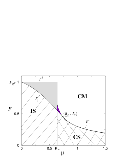
Figure 11: Phase diagram for the piecewise linear pinning force, $Y(x)=-x/\pi$ (see Fig. (1b)). The lightly shaded portion is the coexistence region of the IS and CM phase ($\mu<\mu_{u}$) and the smaller, darkly shaded region, is where the CS and CM phases coexist ($\mu_{u}<\mu<\mu_{e}$). The depinning lines $F_{\uparrow}^{i}=F_{\rm sp}$ and $F_{\uparrow}^{c}$ have been obtained analytically and confirmed by numerics. The boundary $F_{\downarrow}$ where the system repins was obtained numerically. The point $(\mu_{e},F_{e})$ marks where the static-moving transition changes from hysteretic to continuous. The boundary between the IS and CS phases is $F$ independent and lies at $\mu=\mu_{u}$.

For $\mu<\mu_{u}$ the static phase is incoherent and the depinning transition is hysteretic in both $v$ and $r$, as shown in the top two frames of Fig. 12. The system depins at $F_{\rm sp}$ when the drive is ramped up adiabatically from the static phase, but repins at the lower force $F_{\downarrow}$ when the force is ramped back down from the sliding state. The line $F_{\downarrow}$ has been obtained by numerical simulation of the mean field model. The numerics have also revealed that a small region of hysteresis persists for $\mu>\mu_{u}$, although the static phase is coherent here. The behavior of $v$ and $r$ in this region is shown in the two mid frames of Fig. 12. Finally, for $\mu>\mu_{e}$ (where $\mu_{e}$ is the value of the coupling above which the static-moving transition is elastic in nature) the depinning is continuous, as shown in the bottom frames of Fig. 12. The values of $\mu_{e}$ and $F_{e}$ are defined via $F_{\uparrow}^{c}(\mu_{e})=F_{\downarrow}(\mu_{e})=F_{e}$. Finally, the depinning threshold $F_{\uparrow}^{c}$ is nonzero and finite for all $\mu$, i.e., $\mu_{T}=\infty$. This is a general property of discontinuous pinning forces, to be contrasted with the behavior observed for continuous pinning forces, such as the sinusoidal one studied by Strogatz and collaborators. Strogatz

Figure 12: Mean velocity $v$ and coherence $r$ as functions of the driving force $F$ for the piecewise linear pinning force. The curves are obtained numerically by first ramping $F$ from zero to a value well within the sliding state ($F=1.2$), and then decreasing $F$ back down to zero, while holding $\mu$ constant. The top frames show the behavior for $\mu=0.25$, where the initial static state is incoherent: this state starts sliding at the single-particle depinning force $F_{\rm sp}=1$ and repins at a lower force $F\approx 0.88$. The mid frames display the results for an initially coherent static state ($\mu=0.64>\mu_{u}$), which still displays hysteresis, both in $v$ and $r$. The bottom frames are for $\mu=1.0$, which has an initial coherent state and undergoes continuous depinning.

Before closing this subsection, we must address the possibility an of incoherent moving (IM) phase. Strogatz and collaborators Strogatz found that an IM phase is always unstable for a sinusoidal pinning potential. It can be shown that this remains true for other continuous pinning forces. The situation is less clear for discontinuous pinning forces. In Appendix D we present the details of a short time ($t=0$) stability analysis for the IM phase for any $Y(x)$. This analysis will tell us something about the long time, steady state limit, provided $r(t)$ is a monotonic function of time. This analysis predicts a range of stability for the IM phase for discontinuous pinning forces, provided the jump discontinuity at $x=\pi$ is taken into account when preparing the system. However, simulations show that $r(t)$ is in general not monotonic and that the strength of the perturbation needs to be decreased with system size in order to observe the IM phase, suggesting that the perturbative short-time analysis is simply not valid in this case. Finally, if a narrow distribution of pinning strengths $h$ is introduced, we find numerically the IM phase to be unstable. Given these numerical findings, we believe that the IM phase is generally unstable in mean field theory.

V.2 Hard Cubic Pinning Force

The phase diagram for a hard cubic pinning force, given by Eq. (34) with $c>0$ (see Fig. 1(d)) is shown in Fig. 13 for $a=c=1/(\pi+\pi^{3})$.

Figure 13: Phase diagram in the coupling-drive ($\mu$-$F$) plane for a hard cubic pinning force of the type shown in Fig. (1a). The form of the pinning force $Y(x)$ is given by Eq. (34), with $a=c=1/(\pi+\pi^{3})$. The regions of IS-CM, CS-CM and IS-CS-CM coexistence are shown in light, medium and dark gray, respectively. The incoherent and coherent depinning lines are denoted by $F_{\uparrow}^{i}$ and $F_{\uparrow}^{c}$ respectively. The repinning line is denoted by $F_{\downarrow}$. The coherent depinning line and the repinning line join at $(\mu_{e},F_{e})$. Beyond this point the static-moving transition is continuous. The curves $\mu_{u}(F)$ and $\mu_{d}(F)$ are the values of the coupling at which the static system makes the transition to and from finite coherence states, respectively. There curves join at $(\mu_{\rm h},F_{\rm h})$ where the IS-CS transition becomes continuous.

Though the general topology is similar to that of the phase diagram for the piecewise linear force, the history dependence is significantly more complicated. A first difference is that the transition between the IS and CS phases is now continuous for $F<F_{h}$, with $F_{\rm h}$ given by Eq. (38), and hysteretic for $F>F_{\rm h}$. For the parameter values displayed in Fig. 13 the value of $F_{\rm h}$ is very small, but still finite. A second new feature of the phase diagram is the presence of a small region (darkest gray in Fig. 13) where all three phases coexist.

The strong history dependence is manifested in the macroscopic response and includes reentrant behavior for fixed $\mu$ or $F$ histories. The mean velocity and coherence are plotted as a function of (increasing, then decreasing) driving force for a few typical values of $\mu$ in Fig. 14. The pinning force is given by $Y(x)=-(x+x^{3})/(\pi+\pi^{3})$. The top frames show a simple hysteretic depinning transition for a system prepared in the incoherent static state at $F=0$, similar to that seen for a linear pinning force. The middle row of frames display the more complicated history that results when the system is prepared in a coherent static state at $F=0$, with $\mu=0.5$. The velocity shows a single hysteresis loop, but the plot of coherence $r$ shows first a decrease and then a jump to the incoherent state as the force is increased, followed by a jump back to a finite value when bulk depinning takes place. In this case both the regions of IS-CS and IS-CM coexistence are crossed when $F$ is ramped up. The IS-CS transition occurs as the phases are pushed away from their zero-force minima to regions of the pinning potential with higher curvature, which makes the coherent state unstable. Upon decreasing the force, both the coherence and the velocity jump back to zero, then the coherence increases again as the force is decreased. The jumps in coherence when $F$ is ramped down occur at values of $F$ different from those where the coherence jumps during the ramp up. For rather specific values of $\mu$, even more baroque histories can be found by crossing the three-phase coexistence regions. An example is shown in the last row of frames in Fig. 14, where $\mu=0.76$. Here, the sequence is CS$\rightarrow$IS$\rightarrow$CM$\rightarrow$CS, which skips the IS phase on decreasing $F$. Note that the velocity vs. drive force curve is relatively unremarkable, showing simple hysteresis in this case. The coherence history is more complicated.

Figure 14: Mean velocity and coherence versus force for the hard potential and various values of $\mu$. Solid lines are used to display the response obtained when $F$ is ramped up from zero, while dashed lines show the jumps in $v$ and $r$ when ramping $F$ back down. The top frames show the hysteretic depinning of a system prepared in the IS phase. For $\mu=0.5$ (mid frames) the system is initially in a coherent ($r\not=0$) static state at $F=0$. As the force is ramped up, the system first crosses the boundary from the CS to the IS phase, where $r$ jumps discontinuously from its initial finite value to zero, while the system remains pinned ($v=0$). At a higher force the system depins by crossing the boundary from the IS to the CM phase and $r$ jumps from zero to a large finite value. The subsequent ramping down of the field goes through this sequence of phases in reverse order, but the jumps occur at distinct values of $F$. The bottom frames describes the complex response that takes place along a path that crosses the dark region of three-phase coexistence. See the text for further description.

Another interesting feature of the phase diagram for the hard cubic pinning force is that at constant $\mu$, a portion of the moving phase lies between the incoherent and coherent static phases. This suggests the possibility of re-entrance in the depinning transition for $\mu>\mu_{e}$. It is not, however, straightforward to prepare the system in the lightly shaded portion of the phase diagram where IS and CM phases coexist and $\mu>\mu_{e}$ The static solution must either be created “by hand” at that location $(\mu,F)$ in phase space or the system can be prepared in the IS phase at a lower value of $\mu$ and the coupling can then be ramped up to the relevant value $\mu>\mu_{e}$. Both the difficulty of preparing the system in the re-entrant state and the re-entrance for a specially prepared state are displayed in Fig. 15. Here both sets of curves correspond to the same value of the coupling strength, $\mu=1.25$. In the top pair of curves the system is prepared in the coherent state at $F=0$. As the force is ramped up adiabatically, the system depins continuously at $F^{c}_{\uparrow}$, where both velocity and coherence change smoothly, with $r$ rapidly approaching its limiting value, $r=1$. The coexistence region is never accessed in this case. In the bottom set of figures, the system is prepared in an incoherent static state at finite $F$, deep inside the coexistence region. The system is then observed to depin as the force is ramped down at constant $\mu$ across the boundary between the coexistence region and the CM phase. Simultaneously, the coherence jumps from zero to a large finite value. Upon further ramping down $F$, the system repins again continuously at $F^{c}_{\uparrow}$.

Figure 15: Both sets of figures show the behavior of velocity and coherence for $\mu=1.25$, but for different initial states. The top frames are obtained by preparing the system in a coherent state at $\mu=1.25$ and $F=0$, and ramping $F$ up to a value above $F^{i}_{\uparrow}$, and then back down to zero. In this case the depinning is continuous. The bottom frames are obtained by preparing the system in an incoherent state at $\mu=1.25$ and $F=0.9$, inside the lightly shaded area of coexistence of CS and CM phases, and then ramping the force down to zero. Note the depinning upon decreasing force in this case and the subsequent repinning.

V.3 Soft Cubic Pinning Force

We distinguish three types of soft cubic pinning forces given by Eq. (34) with $c<0$. These pinning forces and corresponding potentials are shown in Fig. 1: (a) forces that are monotonic over the entire period and do not turn over in the interval $[-\pi,\pi]$; (b) forces that are nonmonotonic over the period and do turn over in the interval $[-\pi,\pi]$, but are discontinuous; and (c) continuous forces, which are obviously nonmonotonic. The phase diagrams for these potentials exhibit qualitative differences as compared to those discussed so far. Specifically, the CS region at non-zero $F$ may or may not extend to $\mu=\infty$ and may not even exist. For most potentials, however, we do find a non-trivial coherent static phase. The only exception is the case of a sinusoidal pinning force studied previously by Strogatz and collaborators, Strogatz where the CS state is unstable.

For monotonic pinning forces, (a), the boundaries $F^{i}_{\uparrow}$ and $F_{\rm sp}$ intersect at a finite positive value $\mu_{*}$ of $\mu$, given by Eq. (37) (see Sec. IV.3 for a full discussion). This results in a portion of the depinning boundary being horizontal on the $\mu$-$F$ plane, as $F^{i}_{\uparrow}=F_{\rm sp}$ for $\mu\leq\mu_{*}$, as shown in Fig. 16. In contrast, if the pinning force is nonmonotonic, (b) or (c), and reaches its maximum within the period, then $\mu*=0$ and the phase boundary has no horizontal portion. This behavior is shown in Fig. 2 for a nonmonotonic, but discontinuous pinning force.

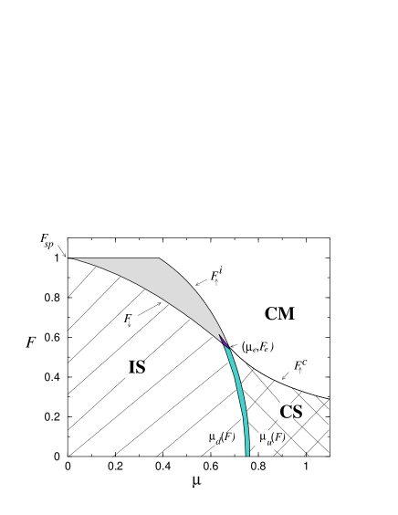
Figure 16: Phase diagram in the coupling-drive ($\mu$-$F$) plane for a soft monotonic cubic pinning force of the type shown in Fig. 1(a). The pinning force $Y(x)$ is given by Eq. (34) with $a=6/(5\pi)$ and $c=-1/5\pi^{3}$. The regions of IS-CM, CS-CM and IS-CS-CM phase coexistence are shown in light, medium and dark gray respectively. The lines $F_{\uparrow}^{i}$ and $F_{\uparrow}^{c}$ are the forces at which the system depins upon increasing the drive from the incoherent and coherent static states respectively. The line $F_{\downarrow}$ is the force at which a moving system stops upon lowering the drive. The coherent depinning line and the repinning line join up at $(\mu_{e},F_{e})$ and the static-moving transition becomes continuous. The curves $\mu_{u}(F)$ and $\mu_{d}(F)$ are the values of the coupling at which the static system makes the transition to and from finite coherence states respectively.

The results for pinning forces of type (c), that are continuous (and therefore must be non-monotonic) have two important features: $\mu*=0$ and $\mu_{T}$ is finite. These features imply, respectively, that there is no horizontal portion to the CS depinning curve and that the system slides at arbitrarily small force whenever the coupling is large, i.e., when $\mu\geq\mu_{T}$. The typical phase diagram for a pinning force of this type is shown in Fig. 17. Figure 18 shows sample $v(F)$ and $r(F)$ plots for this case.

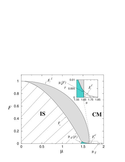
Figure 17: Phase diagram in the coupling-drive ($\mu$-$F$) plane for a soft cubic pinning force of the type shown in Fig. 1(c). The pinning force $Y(x)$ is given by Eq. (34) with $a=3\sqrt{3}/(2\pi)$ and $c=-3\sqrt{3}/(2\pi^{3})$. This choice of parameters gives a non-monotonic and continuous pinning force: the results are to be compared with $Y(x)=-\sin(x)$, another non-monotonic and continuous force. The region of IS-CM coexistence is shown in light gray, while the IS-CS coexistence is shown in medium gray. The lines $F_{\uparrow}^{i}$ and $F_{\uparrow}^{c}$ are the forces at which the system depins upon increasing the drive from the incoherent and coherent static states respectively. The line $F_{\downarrow}$ is the force at which a moving system stops upon lowering the drive. The CS region is very small for these values of parameters, corresponding to $\mu_{T}\approx 1.85$ and $\mu_{d}(0)\approx 1.44$, and it has been magnified in the inset. The CS phase does not exist at finite $F$ for coupling larger than $\mu_{T}$. Shown within this inset is the point $(\mu_{e},F_{e})$ where the $F_{\uparrow}^{c}$ and $F_{\downarrow}$ lines join and the static-moving transition ceases to be hysteretic. The curves $\mu_{u}(F)$ (only visible within the inset) and $\mu_{d}(F)$ are the values of the coupling at which the static system makes the transition to and from finite coherence states respectively.

Figure 18: Mean velocity and coherence, obtained from numerical calculations, for a continuous cubic pinning potential and parameter values given in Fig. 17. The top frames record the hysteretic response of a system prepared in the incoherent state at $\mu=0.8$ and $F=0$, while the bottom frames show the continuous $F=0$ depinning of system prepared in the coherent state at $\mu=1.67$.

At finite drive the CS phase does not extend beyond $\mu=1.84$. For values of the coupling between $\mu_{d}$ and $\mu_{T}$ the CS phase exists at finite drive, albeit only for very small values of $F<F_{\uparrow}^{c}(\mu)\ll 1$. This small region of the phase diagram in Fig. 17 is magnified and shown in the inset. It is interesting to compare the these results with those obtained by Strogatz and collaborators Strogatz for another continuous pinning force, namely $Y(x)=-\sin(x)$. The corresponding phase diagram is shown in Fig. 19. In this case $\mu_{u}=\mu_{T}=2$ and, more significantly, $F_{\uparrow}^{c}(\mu)=0$. This means that the CS phase never exists at finite $F$. Thus, it seems that sinusoidal pinning forces are a special class of more general continuous pinning forces in that they never allow the possibility of a CS phase at finite drive. This difference, while important qualitatively, may not be quantitatively significant given that $F_{\uparrow}^{c}(\mu)$ is always very small.

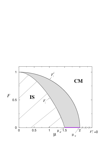
Figure 19: Phase diagram for a sinusoidal pinning force $Y(x)=-\sin(x)$. The IS-CM coexistence region is shaded gray. The $F=0$ region in which the system can only exist in the CS phase is denoted by a series of x’s. The region of IS-CS coexistence is denoted by medium on-axis gray shading. The IS$\rightarrow$CS and IS$\leftarrow$CS phase boundaries are the points $(\mu=\mu_{u}=2,F=0)$ and $(\mu=\mu_{d}\approx 1.49,F=0)$ respectively. The line $F_{\uparrow}^{i}$ is the forces at which the system depins from the incoherent state. The line $F_{\downarrow}$ is the force at which a moving system stops upon lowering the drive.

Finally, for any continuous pinning force, the IM phase is not stable even in the short time analysis. (See Appendix D.) This result is consistent with the findings of Strogatz and collaborators Strogatz as well as our simulations.

VI Averaging over disorder

In this section we discuss the role of the shape of the distribution $\rho(h)$ of pinning strengths on determining the nonequilibrium phase diagram. In the previous sections we restricted ourselves to an infinitely sharp distribution, $\rho(h)=\delta(h-1)$. This choice is appropriate for systems with strong pinning and allows for a direct comparison with the results of Strogatz and collaborators Strogatz . It is easy to show that the nonequilibrium phase diagram of the driven system retains the same qualitative structure for any distribution that is sharply peaked around a finite value of the pinning strength and vanishes below a finite $h_{0}>0$. A broad distribution of pinning strength may, however, qualitatively alter the mean field physics. Broad distributions $\rho(h)$ are of interest to model physical systems with weak pinning. Furthermore, a broad distributions of pinning strengths yields variations of the local stresses in the mean field theory and may give us some insight into the behavior of the system in finite dimensions.

We consider a distribution of pinning strengths $\rho(h)$ that vanishes below a minimum pinning strength $h_{0}\geq 0$. As will become apparent below, it is important to distinguish three class of distributions:

1. distributions that vanish below a finite pinning strength, i.e., $\rho(h)=0$ for $h<h_{0}$, with $h_{0}>0$;

2. distributions with no finite lower bound of the pinning strength, but zero weight at $h=0$, i.e., $h_{0}=0$, and $\rho(0)=0$;

3. distributions with no finite lower bound of the pinning strength, and finite weight at $h=0$, i.e., $h_{0}=0$, but $\rho(0)>0$.

The nonequilibrium phase diagram depends qualitatively on whether or not the lower bound $h_{0}$ is finite. If the distribution of pinning strengths $\rho(h)$ vanishes below a minimum pinning strength $h_{0}>0$, the single particle depinning threshold $F_{\rm sp}$ remains finite and the system exists in an IS phase for $F<F_{\rm sp}$. When $h_{0}=0$, the single particle depinning threshold vanishes and the IS state can only be stable at $F=0$.

If the IS phase exists, its stability can be analyzed for an arbitrary distribution $\rho(h)$ by the perturbation theory described in Sec. IV. For arbitrary $h$, the static force balance equation has the form

$$0=F-u\sin(\theta-\psi)+hY(\theta-\beta)\;,$$ (46)

with the self-consistency condition given by Eq. (6). Clearly this equation is identical to the equation studied in Sec. IV for $h=1$, provided we rescale both the driving force $F$ and the coupling strength $u$ by the pinning strength $h$. We can then carry out the perturbation theory described in Sec. IV as a perturbation theory in powers of $u/h$, provided of course $u<<h_{0}$. This shows that the perturbation theory breaks down when $h_{0}\rightarrow 0$. Furthermore we must require $F<F_{\rm sp}$, which is a necessary condition for the existence of the IS phase. Proceeding precisely as in Sec. IV and using the same notation, we obtain an expression for the coherence $r$ as a power series in $u/h$, given by

$$r=f(u,F)=\int dh\rho(h)[ r_{1}(F/h)\frac{u}{h}+r_{2}(F/h)\Big{(}\frac{u}{h}\Big{)}^{2}+$$

$$r_{3}(F/h)\Big{(}\frac{u}{h}\Big{)}^{3}+\dots]\;,$$ (47)

with

$$r_{1}(F/h) = {1\over 2{\tilde{a}}(F/h)}\;,$$ (48a)

$$r_{2}(F/h) = 0\;,$$ (48b)

$$r_{3}(F/h) = {3\over 8}\frac{{\tilde{a}}(F/h){\tilde{c}}(F)-2\big{[}{\tilde{b}}(F/h)\big{]}^{2}}{{\tilde{a}}(F/h)^{5}}\;,$$ (48c)

and

$${\tilde{a}}(F/h) = Y^{\prime}(\delta_{0})\;,$$ (49a)

$${\tilde{b}}(F/h) = Y^{\prime\prime}(\delta_{0})/2\;,$$ (49b)

$${\tilde{c}}(F/h) = Y^{\prime\prime\prime}(\delta_{0})/6\;.$$ (49c)

The boundary of stability of the IS phase, $\mu_{u}(F)$, is obtained like before by solving the implicit equation $r(\mu,F)=f(u=\mu r,F)$ with $f(u,F)$ given by Eq. (47), with the result

$$\mu_{u}(F)=2\bigg{[}\int\rho(h)\frac{1}{h\tilde{a}(F/h)}\bigg{]}^{-1}\;.$$ (50)

If the distribution $\rho(h)$ vanishes below a finite minimum pinning force $h_{0}>0$, then $\mu_{u}$ remains finite and there is a range of $\mu$ and $F$ where the IS phase is stable. Conversely, if $h_{0}\rightarrow 0$, the integral in Eq. (50) may diverge, yielding $\mu_{u}=0$. Below we will treat in detail the case of a piecewise linear pinning force, with $Y(x)=-ax$. In this case Eq. (50) reduces to

$$\mu_{u}=2a\bigg{[}\int dh\frac{\rho(h)}{h}\bigg{]}^{-1}\;.$$ (51)

For concreteness, we consider a distribution of the form

$$\rho(h)=(h-h_{0})^{\alpha}\,e^{-(h-h_{0})}\;,\hskip 14.45377pth\geq h_{0}\;,$$

$$\rho(h)=0\;,\hskip 14.45377pth<h_{0}\;,$$ (52)

with $h_{0}>0$ and $\alpha>0$. This form encompasses the three classes of distribution functions introduced at the beginning of the section. We can then obtain the boundary of the IS phase for a piecewise linear pinning force by evaluating the integral on the right hand side of Eq. (51). For distributions of the first class, corresponding here to $h_{0}>0$ and $\alpha=0$, we find that $\mu_{u}$ is finite at finite $F$ and it is given by $\mu_{u}=2ae^{h_{0}}E_{1}(h_{0})$, where $E_{1}(x)$ is the exponential integral. For this type of distribution it can be shown that the nonequilibrium phase diagram remains qualitatively similar to the one obtained for the sharply pinned distribution, $\rho(h)=\delta(h-1)$, even for all types of pinning forces studied in Sec. V. When $h_{0}\rightarrow 0$ the perturbation theory breaks down and the existence of a finite value of $\mu_{u}$, even at $F=0$, depends on the form of $\rho(h)$ for $h\rightarrow 0$. For distributions of the second class, with $h_{0}=0$, but $\rho(0)=0$, it can be shown that $\mu_{u}$ is finite at $F=0$, but vanishes at all finite $F$. In this case there is an IS-CS transition at $F=0$, which is a remnant of the transition seen at finite $F$ for the case of an infinitely sharp pinning strength distribution. For instance, for $\rho(h)=he^{-h}(\alpha=1)$, there is an IS-CS transition at $F=0$ and $\mu_{u}\simeq 0.27$. Finally, for distributions in the third class, with $\rho(0)>0$, it can be shown that $\mu_{u}$ vanishes as $1/\ln(1/h_{0})$ when $h_{0}\rightarrow 0$. For such distributions, there is no IS phase even at $F=0$. The phase diagrams for this class of distributions of pinning strength are qualitatively different from those presented in Sec. V for all pinning forces. An example is shown in Fig. 20 for the piecewise linear pinning force and $\rho(h)=e^{-h}$. This phase diagram has been obtained numerically. In the limit of large system sizes and adiabatically slow ramp rates $dF/dt$, no IS phase is observed even at $F=0$. The small region of hysteresis in the transition between the CS and CM phases is also washed out by the disorder averaging. The depinning curve $F^{c}_{\uparrow}$ displays a broad maximum at a finite $\mu$ and vanishes as $\mu\rightarrow\infty$.

Figure 20: Phase diagram in the $\mu-F$ plane for a piecewise linear pinning force, with $a=1/\pi$ and $c=0$, and $\rho(h)=e^{-h}$. The depinning curve has been obtained numerically for a system with $N=1024$ and a ramp rate of $dF/dt=10^{-6}$.

In general, the numerical simulations show that a broad distribution of pinning strengths with vanishing $h_{0}$ always washes out the IS phase and any hysteresis of the depinning transition. Whether this behavior persists in finite dimensions remains an open question.

VII Discussion

In this paper we have used a combination of analytical and numerical techniques to study the nonequilibrium mean field phase diagram of a model of an extended systems with phase slips driven through disorder. For uniform pinning, we generically find two stable static phases and a single moving phase. Both incoherent (IS) and coherent static (CS) phases are possible, as well as regions where the two phases coexist. The moving phase, in contrast, is always coherent (CM) in mean field theory. (An incoherent moving phase can be prepared by using special initial conditions, but does not appear to be stable.) Coexistence of two, or even three, of these phases can occur depending on the system preparation; this coexistence results in hysteretic transitions. Such a variety of phases was not found for the case of a sinusoidal pinning force analyzed earlier,Strogatz where only the IS and CM phases were found. While a discontinuity in the pinning force is not required for the existence of the new CS phase at large values of the coupling constant $\mu$, a jump discontinuity in the pinning force does increase the range of $F$ and $\mu$ over which the CS phase is observed. This is because discontinuity in the pinning force makes it more difficult for the system to depin, so that the static pinned phases can exist up to large coupling strengths, where the system is forced to acquire long range coherence. Once the system has become coherent, and therefore more rigid, the depinning threshold decreases with increasing $\mu$, but remains finite for all finite values of the coupling strength and only vanishes for $\mu\rightarrow\infty$. For a continuous pinning forces, on the other hand, the depinning threshold vanishes above a finite value of $\mu$.

In order to make some contact with particle simulations and with experiments, it is useful to discuss the mean field phase diagram in terms of the disorder strength $h$ and the driving force $F$, rather than in the $(\mu,F)$ plane as done so far. In most particle simulations it is the strength of the disorder that is most easily varied rather than the strength of the coupling. Disorder is also a crucial control parameter in many experimental systems. For instance,varying the applied magnetic field in current-driven vortex lattices has the effect of varying the strength of the disorder. At high fields the vortex lattice becomes softer and can better adjust to disorder. Increasing the magnetic field therefore corresponds to an effective increase of the disorder strength. Fig. 21 shows the mean field phase diagram in the $(h,F)$ plane for the discontinuous soft cubic pinning force shown in Fig. 1b. The corresponding phase diagram in the $(\mu,F)$ plane was shown in Fig. 2.

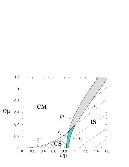
Figure 21: Phase diagram, redrawn in the disorder-drive plane, for a discontinuous soft cubic pinning force of the type shown in Fig. 1b and $\rho(h)=\delta(h-1)$. The disorder $h$ and drive $F$ are normalized by the strength of the phase-slip interaction, $\mu$. The parameter values and the symbols are the same as in Fig. 2.

When the disorder is weak relative to the strength of the coupling $\mu$ the static phase is coherent. At strong disorder the static phase is incoherent. The transition between the coherent and incoherent static phases at fixed $\mu$ is hysteretic with a region of coexistence of the two phases. At weak disorder there is a continuous “elastic-like” depinning transition from the CS to the CM phase. At large disorder the static phase is incoherent and degrees of freedom depin independently at the single particle depinning threshold, $F^{i}_{\uparrow}$. The moving system immediately acquires long-range correlations, becoming much stiffer and harder to pin. As a result, when the force is ramped down the CM state repins at the lower force $F_{\downarrow}$. The qualitative features of this phase diagram are remarkably similar to those obtained by Olson and collaborators Olson01 in a numerical simulation of a model of a current-driven layered superconductors, with magnetically interacting pancake vortices. At weak disorder these authors find that the layers are coupled and the system forms a coherent three-dimensional static phase, with long-range correlations along the direction normal to the layers, which depins continuously. At strong disorder the static state consists of decoupled two-dimensional layers. When the driving force is ramped up from this incoherent static state, the layers depin independently at the single-layer depinning threshold and the transition is hysteretic. One difference between our mean field model and the numerical model studied by Olson et al. is the absence, in our model, of an incoherent moving phase. In the layered superconductor at strong disorder the layers remain decoupled upon depinning up to a second, higher threshold force where a dynamical re-coupling transition occurs. Finally, these authors also observe a sharp increase in the depinning threshold at the crossover or transition from continuous to hysteretic depinning, not unlike that shown in Fig. 21. A strong crossover from elastic to plastic with increasing disorder strength, with an associated sharp rise of the depinning threshold, has also been seen in a variety of two dimensional simulations, such as those by Faleski, et al.FMM Macroscopic hysteresis has not, however, been observed in these two-dimensional models. Our work suggests that mean field models with strong disorder tend to overestimate hysteresis. In mean field there is no range of correlation lengths and hysteresis will always occur when the system is driven from a strongly pinned incoherent phase, where all degrees of freedom depin independently at the single particle depinning threshold. Upon depinning, the system acquires long range order and becomes therefore much stiffer, so that when the force is ramped down it can remain in the sliding state down to much lower values of the driving force.

Early transport experiments on current-driven vortices in NbSe₃ showed S-shaped IV characteristics at high magnetic fields with a peak in the differential resistance as a function of driving current.fingerprint Other puzzling effects were observed in the region of the peak, including unusual frequency dependence of the ac response and fingerprint phenomena. These experimental findings were originally interpreted in terms of plastic depinning of the vortex system and macroscopic coexistence of disordered and ordered bulk vortex phases. This interpretation was corroborated by a number of simulations in two-dimensions, where the crossover from elastic to plastic depinning is clearly seen as a function of disorder strength. For strong disorder the system exists in a disorder static phase that depins plastically and then undergoes a dynamical ordering transition to a moving ordered phase. The peak in the differential resistance corresponds to such a dynamical ordering transition and in simulations is clearly associated with a sharp drop in the number of topological defects in the driven lattice. More recent experiments have suggested, however, that the disordered phase is a metastable phase that is injected at the sample’s edges and then anneals into the stable elastic phase as it gets driven into the sample. paltiel ; Paltiel02 ; marchevsky This interpretation has been confirmed by comparing transport experiments in the conventional strip geometry, where the edge effect is always present, to experiments in a Corbino disk geometry, where the vortices are driven to move in concentric circular orbits in a disk-shaped sample, eliminating boundary effects. Although there is mounting experimental evidence that these edge contamination effects may indeed control much of the vortex dynamics observed in experiments, the comparison with simulations, where coexistence of bulk ordered and disordered phases is routinely observed, remains puzzling. Of course one important difference is that most of the simulations are carried out at zero or very low temperature, where the disordered phase may be artificially stabilized.

Substantial phase slip effects have also been observed in CDW systems, especially at the contacts Thorneexpt , and have been associated with the “switching” observed in certain materials. The reported correlation between broadband noise and macroscopic velocity inhomogeneities also supports the idea that in these systems the dynamics may be dominated by large scale plasticity. broadband While the switching itself has also been explained as arising from the presence of normal carriers levy92 , phase slips seem crucial to account for the correlation between broadband noise and macroscopic velocity inhomogeneities.

Finally, similar behavior has also been observed in colloids driven over a disordered substrate. Pertsinidis and Ling Ling have studied experimentally single layers of two-dimensional colloid crystal driven by an electric field over a disordered substrate. They observe plastic-like or filamentary flow of the colloids, with a velocity-force curve that is always convex upward and shows no hysteresis. Langevin simulations by Reichhardt and Olson ReichhardtOlson find a sharp crossover from elastic to plastic depinning as the strength of substrate is increased. Though the direct applicability of our mean field model and results to experimental systems remains to be proven, this work lays out a detailed foundation for understanding the role of phase slips and topological defects on the dynamics of driven disordered systems. Preliminary numerical studies of the phase slip model in three dimensions, with a sinusoidal pinning potential, suggest that the depinning transition may not be hysteretic in the thermodynamic limit. This is similar to what suggested by studying the mean field with a broad distribution of pinning strengths, as shown in Fig. 20, where the distribution of pinning forces the incoherent static (IS) phase. Clearly more work is needed to establish if such a finding is generic in finite dimensions. An important open question is whether the transition from elastic to plastic depinning (with or without macroscopic hysteresis) is a crossover or is associated with some type of tricritical point, as suggested by the present and other mean field models.

This work was supported in part by NSF grants DMR-9730678, DMR-0109164 and DMR-0305407.

Appendix A Coherence at $F=0$

In this appendix we describe the calculation of the coherence $r(\mu)$ of static states at $F=0$. First we derive an expression for the function $f(u)$ defined in Eq. (9) for an arbitrary pinning force, $Y(\delta)$. Once $f(u)$ is known, the coherence is then obtained by solving the self-consistency condition, $r=f(\mu r)$. The calculation is complicated by multivalued solutions to the self-consistency equations, which leads to multiple metastable states. A consistent selection principle is applied, namely, choosing the coherence $u$ to be maximal, given $\mu$. The range of available metastable states is also used to determine $\mu_{T}$, the value of coupling above which the depinning field is zero.

A.1 Change of variables

As discussed in Section III.3, it is convenient to perform a change of variables in Eq. (9) and integrate over $\delta$ rather than over the random phase $\beta$. The function $f(u)$ is then given by

$$f(u)={1\over 2\pi}\int_{-\pi}^{\pi}d\delta\left({\partial\beta\over\partial\delta}\right)\cos[\delta+\beta(\delta,u)]\;,$$ (53)

where $u=\mu r$. Since $Y(\delta)$ is $2\pi$ periodic, the integration in Eq. (53) can be carried out over any $2\pi$ interval. Here we choose the interval $[-\pi,\pi]$. The change of variable allows us to evaluate $f(u)$ analytically as the force balance equation, Eq. (8), while transcendental in $\delta(\beta,u)$, is simply a linear equation in the phase $\beta(\delta,u)$. We can therefore immediately write the solution $\beta(\delta,u)$ of Eq. (8), substitute it in Eq. (53), and evaluate the integral to obtain $f(u)$. As we will see below, the only difficulty in carrying out this program is that the phase $\delta(\beta,u)$ is generally a multivalued function of $\beta$. Therefore care must be taken in selecting the portion of the curve that must be included in the integral. The choice is dictated by the requirement that the imaginary part of the self consistency condition, which now reads

$$0={1\over 2\pi}\int_{-\pi}^{\pi}d\delta\left({\partial\beta\over\partial\delta}\right)\sin[\delta+\beta(\delta,u)]\;,$$ (54)

be satisfied, and that the phase $\delta(\beta)$ span a full $2\pi$ interval in $\beta$.

For static solutions and $F=0$ the balance equation (8) can be written as

$$\sin(\delta+\beta)=\frac{Y(\delta)}{u}\;.$$ (55)

Since $|\sin(\delta+\beta)|\leq 1$, the right hand side of Eq. (55) must also be bounded in magnitude by one. This means that all solutions to Eq. (55) must satisfy

$$-\delta_{max}(u)\leq\delta\leq\delta_{max}(u)\;,$$ (56)

where $\delta_{max}(u)$ is defined by

$$|Y(\delta_{\max})|=u\;,$$ (57)

or $\delta_{max}(u)\equiv|Y^{-1}(u)|$, with $Y^{-1}$ denoting the inverse function. Note that if $Y(\delta)$ is non-monotonic in the interval $[-\pi,\pi]$, as it is for instance the case for the soft cubic potential shown in Fig. 1(b), then for $u>|Y(\pi)|$ there are two possible values of $|Y^{-1}(u)|$ in the range $[0,\pi]$. In this case $\delta_{max}$ is defined as the smallest of these two values. At the end of this Appendix we will discuss the relevance of the second solution and demonstrate that it corresponds an unstable state.

A.2 Metastable states

For every fixed value of $u$, there is in general an infinite set of solutions for the phase $\delta$ in the range $[-\delta_{max},\delta_{max}]$. The corresponding solutions for the phase $\beta$ as a function of $\delta$ can be enumerated by indexing them with an integer, $n$. They are given by

$$\beta_{n}(\delta,u)=-\delta+n\pi+(-1)^{n}\sin^{-1}(Y(\delta)/u)\;,$$ (58)

where we only consider values of the function $\sin^{-1}(x)$ in the range $[-\pi/2,\pi/2]$. Since the calculation of $\beta_{n}(\delta,u)$ and $\delta(\beta,u)$ is carried out at fixed $u$, from here on we will simply omit the $u$ dependence in the argument of these functions. The typical behavior of the phase $\delta$ as a function of $\beta_{n}$, for $-2\leq n\leq 2$, is shown in Fig. 5.

The integral in Eq.(53) must span a full period (in $\beta$) of the $\delta(\beta)$ curve. As evident from Fig. 5, this always corresponds to a pair of consecutive even-odd sections. Here we choose to work with the $n=0$ section, and the upper and lower halves of the $n=-1$ and the $n=1$ sections, respectively. This choice is equivalent, for instance, to that of the $n=0$ and the full $n=-1$ sections (or $n=0$ and $n=1$), but it has the advantage of being symmetric about the origin. The chosen portion of the $\delta(\beta)$ curve is displayed in Fig. 22 for three different values of $u$. The figure shows how the phase becomes multivalued as $u$ is increased.

Figure 22: The figure shows the behavior of the phase $\delta(\beta)$ for three values of $u$. The $n=\pm 1$ half-sections are dashed, while the $n=0$ section is solid. Curve (a) corresponds to $u\leq a$ and is single valued. Curves (b) and (c) are both multivalued and correspond to (b) $a<u\leq Y(\pi/2)$ and (c) $u>Y(\pi/2)$. The section $\beta_{0}$ ends at the points $\pm\delta_{max}$, where the half sections $\beta=\mp 1$ begin. For curve (b) these points lie within the portion of the curve that must be included in the integral to determine $f(u)$. For curve (c) they lie outside. $\delta_{*}$ denotes the non-zero value of the phase at $\beta=-\pi$.

For $u\leq a$, with $a$ the linear slope of the pinning force $Y(\delta)$ at $\delta=0$, the phase $\delta$ is single-valued, as in curve (a) of Fig. 22. In this case integrating over a full period in $\beta$ is equivalent to integrating over the entire curve, consisting of the full $n=0$ central section (solid) and the two $n=\pm 1$ half sections (dashed). Making use of the symmetry of the integrand about $\delta=0$, we obtain

$$f(u) = {1\over\pi}\int_{0}^{\delta_{max}}d\delta\left({d\beta_{-1}\over d\delta}\right)\cos[\delta+\beta_{-1}(\delta,u)]$$ (59)

$$+ {1\over\pi}\int_{\delta_{max}}^{0}d\delta\left({d\beta_{0}\over d\delta}\right)\cos[\delta+\beta_{0}(\delta,u)]\;.$$

Upon substituting the expressions for $\beta_{-1}(\delta)$ and $\beta_{0}(\delta)$ from Eq. (58) in Eq. (59), we obtain

$$f(u)={2\over\pi}\int_{0}^{\delta_{max}}d\delta~{}\sqrt{1-[Y(\delta)/u]^{2}}\;,\hskip 18.06749ptu\leq a\;.$$ (60)

When $\delta(\beta)$ is single valued, the integral in Eq. (10) over the entire period gives zero, so that the imaginary part of the self consistency condition is satisfied.

When $u\geq a$, the phase $\delta$ is multivalued, as exemplified in cases (b) and (c) in Fig. 22. In this case one can no longer simply integrate over the full curve in the range $\beta\in[-\pi,\pi]$. Rather, one must select a portion, of measure $2\pi$ in $\beta$, that satisfies the imaginary part of the self consistency condition, Eq. (54). As discussed in Sec. III.3 we choose the portion of the curve corresponding to the metastable states that would be accessed by adiabatically increasing $u$ from zero. For $\psi=0$, this choice corresponds to the connected part of the $\delta(\beta)$ curve lying between $\beta=-\pi$ and $\pi$. This choice is odd about the origin and therefore automatically satisfies Eq. (54). The phase $\delta$ now has two values at $\beta=\pi$, $\delta=0$ and $\delta=\delta_{*}$, which is defined implicitly as the nonzero root of the equation

$$-Y(\delta_{*})=u\sin(\delta_{*})\;.$$ (61)

The value $\delta_{*}$ is the desired upper limit in the integration over $\delta$ in Eq. (53). When $a\leq u\leq Y(\pi/2)$, corresponding to curve (b) in Fig. 22, the root $\delta_{*}$ is smaller than $\delta_{max}$ and the portion of the curve to be included in the integrand spans the entire $\beta_{0}(\delta)$ section (solid line) and those parts of the $\beta_{\pm 1}(\delta)$ half sections (dashed) that lie within $\beta=[-\pi,\pi]$. For this range of $u$ values we find

$$f(u) = {2\over\pi}\int_{0}^{\delta_{max}}d\delta~{}\sqrt{1-(Y(\delta)/u)^{2}}-{Y(\delta_{*})\over u\pi}$$ (62)

$$- {1\over\pi}\int_{0}^{\delta_{*}}d\delta~{}\sqrt{1-(Y(\delta)/u)^{2}}\;,$$

$$\hskip 72.26999pta\leq u\leq|Y(\pi/2)|\;.$$

At $u=|Y(\pi/2)|$, $\delta_{*}=\delta_{max}$. For $u>|Y(\pi/2)|$, corresponding to the situation illustrated in curve (c), $\delta_{max}$ exceeds $\delta_{*}$ and the portion of the curve to be included in the integrand only spans that part of the $\beta_{0}(\delta)$ section (solid) that lies in $\beta\in[-\pi,\pi]$, as seen from Fig. 22. In this case we obtain

$$f(u) = {1\over\pi}\int_{0}^{\delta_{*}}d\delta~{}\sqrt{1-(Y(\delta)/u)^{2}}-{Y(\delta_{*})\over u\pi}\;,$$ (63)

$$\hskip 57.81621ptu\geq|Y(\pi/2)|\;.$$

The three equations, Eqs. (60), (62) and (63), give the function $f(u)$ at all $u$ for an arbitrary pinning force, $Y(\delta)$. It can be shown that when Eq. (60) is expanded for small $u$, the perturbative result, Eq. (19), is recovered.

For a piecewise linear pinning force, with $Y(\delta)=-a\delta$ for $-\pi\leq\delta\leq\pi$, the integrals in Eqs. (60), (62) and (63) can be evaluated analytically, with the result

$$f(u)=\begin{cases}{u\over 2a},&u\leq a,\\ {u\over 2a}+{\delta_{*}\over 2\pi}\left({2a\over u}-{u\over a}-\cos\delta_{*}\right),&a<u\leq a\pi/2,\\ {\delta_{*}\over 2\pi}\left({2a\over u}+{u\over a}+\cos\delta_{*}\right),&u<a\pi/2,\end{cases}$$ (64)

where $\delta_{*}=(u/a)\sin(\delta_{*})$. The coherence $r$ is then determined by the solution of $r=f(\mu r)$. For $u\leq a$ the equation for the coherence is $r=\mu r/\mu_{u}$, where $\mu_{u}=1/(2a)$. If $\mu\neq\mu_{u}$, the only solution is $r=0$. For $\mu=\mu_{u}$ the equation is satisfied by any nonzero value of $r$ consistent with $u\leq a$, or equivalently $r\leq 1/2$. Thus, at $\mu=\mu_{u}$ the coherence jumps discontinuously from zero to the value $r_{0}=1/2$. By expanding $f(u)$ for $u\rightarrow a^{+}$ we find that for $\mu\gtrsim\mu_{u}$,

$$r-r_{0}\propto(\mu-\mu_{u})^{2\over 5}\;.$$ (65)

The full solution $r$ as a function of $\mu$ is shown in Fig. 6.

We now return to the question of the existence of solutions $\delta(\beta)$ outside the range $[-\delta_{max},\delta_{max}]$. This is relevant for pinning forces $Y(\delta)$ that are non-monotonic in the interval $[-\pi,\pi]$. For such pinning forces the Eq. (61) has two nonvanishing solutions. The smallest of these two solutions, $\delta_{*}$ defines the range of phases that have been used in the calculation of the coherence described above. Denoting the largest of the two solutions by $\delta_{u}$, we note that for $u>|Y(\pi)|$ there will also be solutions for the phase $\delta$ lying in the ranges $[\delta_{u},\pi]$ and $[-\pi,-\delta_{u}]$. Examples of such solutions are shown in Fig. 23 for the soft cubic pinning force. The solutions outside the range $-\delta_{max}\leq\delta\leq\delta_{max}$ are the top and bottom branches in the figure. It can be shown that such solutions are always unstable, while the center branch is stable. This is easily seen by plotting the total force $F_{tot}=-u\sin(\delta+\beta)+Y(\delta)$ acting on a domain versus the phase $\delta$, for a fixed value $\beta$. The stable solutions of the force balance equation are the zeros of $F_{tot}(\delta)$ with a negative slope, so that they correspond to minima of the total potential. The zeros with a positive slope are maxima of the potential and therefore represent unstable solutions. Of the two zeros shown for instance in Fig. 24 for $\beta=\pi/2$, only the left solution, which lies in the range $[-\delta_{max},\delta_{max}]$ is stable, while the right one is outside this range and is unstable. Changing the value of $\beta$ would simply shift the curve of $F_{tot}$ along the $\delta$ axis, with the stable root always remaining inside the interval $[-\delta_{max},\delta_{max}]$.

Figure 23: The figure shows the phase $\delta$ versus $\beta_{n}$ at $u=0.8$, for $n=0,\pm 1,\pm 2$, for the continuous pinning force of Fig. 1(c), with $a=3\sqrt{3}/(2\pi)$ and $c=-3\sqrt{3}/(2\pi^{3})$. The upper and lower branches, lying outside the range $[-\delta_{max},\delta_{max}]$ are unstable, while the central branch is stable.

Figure 24: Plot of $F_{\bf tot}$ versus $\delta$ for $\beta=\pi/2$, $u=0.8$ for the continuous pinning force of Fig. 1(c), with $a=3\sqrt{3}/(2\pi)$ and $c=-3\sqrt{3}/(2\pi^{3})$. The equation $F_{\bf tot}=0$ has two solutions. The left solution, with negative slope is stable, while the right one, with positive slope, is unstable.

A.3 Derivation of $\mu_{T}$

The number of metastable static states available to the system plays an important role in determining the depinning threshold. In general the system can exist in a large number of static metastable states and the function $\delta(\beta)$ becomes more multivalued as $u$ increases, as shown in Fig. 22. The number of metastable states is not, however, a monotonic function of $u$ as only values of $\delta$ lying in the interval $[-\pi,\pi]$ are acceptable solutions. The number of available metastable states increases with increasing $u$ until $\delta_{max}(u)=\pi$, corresponding to $u=|Y(\pi)|$. As $u$ is increased beyond $|Y(\pi)|$ the number of metastable states decreases. When an infinitesimal force is applied, all the phases are pushed forward and an infinitesimal number of static metastable states becomes unstable as they can no longer satisfy the self-consistency condition. The system remains, however, pinned, provided there exist other static states that are still metastable. When $\delta_{*}(u)=\pi$, the situation changes as there is only one metastable static solution that becomes unstable as soon as an infinitesimal driving force is applied to the system. The system depins as soon as $F>0$, i.e., the threshold force for depinning is zero.

It can be seen from Eq. (61) defining $\delta_{*}$ that for pinning forces with $|Y(\pi)|>0$, $\delta_{*}<\pi$ for any finite $u$. In this case $\delta_{*}$ approaches $\pi$ only in the limit $u\rightarrow\infty$. Since $r$ is always finite, it is only in the limit of infinite $\mu$ that the system approaches a perfectly ordered floating state and the depinning threshold force goes to zero. For continuous pinning forces with $Y(\pi)=0$, $\delta_{*}=\pi$ at a finite value of $u=u_{T}\equiv Y^{\prime}(\pi)$. For $u\geq u_{T}$, the system has only a single, albeit partially disordered, state available. This state becomes unstable upon application of an infinitesimal driving force, and the system begins to slide. In other words, the threshold for depinning vanishes for all $u\geq u_{T}$ or, equivalently, all $\mu\geq\mu_{T}=u_{T}/f(u_{T})$. Using Eq. (63) we find the value of $\mu_{T}$ displayed in Eq. (23).

Appendix B Depinning force $F_{\uparrow}^{c}(\mu)$

In this appendix we calculate the depinning force $F_{\uparrow}^{c}(\mu)$ for hard and soft cubic pinning forces, of the type sketched in Fig. 1. These forces are given by Eq. (34) with $c>0$ for the hard cubic force and $c<0$ for the soft cubic force. Due to the periodicity of the problem, we can restrict ourselves to any interval of $\delta$ of range $2\pi$. For simplicity we choose again $\delta$ to lie in the $[-\pi,\pi]$ interval. In this interval the force balance equation, with $\psi=0$ is

$$0=F-u\sin(\delta+\beta)+Y(\delta)\;,$$ (66)

and only solutions to Eq. (66) which satisfy $-\pi\leq\delta(\beta,u,F)\leq\pi$ should be considered.

As for the case $F=0$, the transcendental nature of the force balance equation, Eq. (66), can be circumvented by integrating over $\delta$ rather than over the phase $\beta$ in the self-consistency conditions. Solving for $\beta(\delta,u,F)$ gives an infinite set of of solutions, labeled by an integer $n$,

$$\beta_{n}(\delta)=-\delta+n\pi+(-1)^{n}\sin^{-1}\left({Y(\delta)-F\over u}\right)\;,$$ (67)

where $\delta$ is restricted to lie in the range

$$\delta_{min}(u,F)\leq\delta\leq\delta_{max}(u,F)\;,$$ (68)

with

$$\delta_{min}(u,F)\equiv-Y^{-1}(F-u)\;,$$

$$\delta_{max}(u,F)\equiv-Y^{-1}(F+u)\;.$$ (69)

The solution must satisfy the real and imaginary parts of the self consistency condition, given by,

$$r=f(u,F)\;,$$ (70)

$$0={1\over 2\pi}\int_{2\pi}d\delta\left({\partial\beta\over\partial\delta}\right)\sin[\delta+\beta(\delta,u,F)]\;,$$ (71)

with

$$f(u,F)={1\over 2\pi}\int_{2\pi}d\delta\left({\partial\beta\over\partial\delta}\right)\cos[\delta+\beta(\delta,u,F)]\;.$$ (72)

Throughout the analysis we will be considering $\delta(\beta,u,F)$ for fixed values of $u$ and $F$. We will therefore write $\delta=\delta(\beta)$, with the dependence on $u$ and $F$ implied.

As in the case $F=0$, the phase $\delta$ is generally a multivalued function of $\beta$ (see Fig. 25). We consider only the metastable state corresponding to a connected portion of the curve $\delta(\beta)$ in the range $\delta\in[\delta_{L},\delta_{R}]$, and it is this portion that is integrated over in the self-consistency conditions. We focus in this particular state because it is the one that controls depinning. The points $\delta_{L}$ and $\delta_{R}$ bounding this portion are functions of $u$ and $F$ and may in general differ from $\delta_{min}$ and $\delta_{max}$. They are determined by the requirement that the imaginary part of the self-consistency condition, Eq. (71), be satisfied and by the condition that the portion of the function $\delta(\beta)$ bounded by these points span a full $2\pi$ interval in $\beta$, i.e.,

$$\beta(\delta_{L})+2\pi=\beta(\delta_{R})\;.$$ (73)

The details on how the limits of integration are determined and the corresponding portion of the solution for $\beta(\delta)$ is chosen in each case are given below.

Figure 25: The phase $\delta(\beta)$ as a function of $\beta_{n}$ for $-2\leq n\leq 2$ for two sets of values of $(u,F)$, corresponding to single-valued (for $(u=0.1,F=0.2)$) and multi-valued (for $(u=0.35,F=0.2)$) solutions. Even $n$ branches are drawn as solid lines and odd $n$ branches are dashed.

After evaluating the coherence, we can then proceed to compute the force $F_{\uparrow}^{c}(\mu)$ where the static coherent state becomes unstable and the system begins to slide. As $F$ is increased at fixed $u$, the whole $\delta(\beta)$ curve shifts upward and both $\delta_{max}$ and $\delta_{L}$ increase. The number of static metastable states in the range $\delta\in[-\pi,\pi]$ decreases, until at the critical force $F_{\uparrow}^{c}$ only one static metastable state remains. This occurs where the largest value of $\delta$ on the connected portion, denoted by $\delta_{u}$, reaches $\pi$, i.e.,

$$\delta_{u}(u,F_{\uparrow}^{c})=\pi\;.$$ (74)

Upon further increasing $F$ the system depins. Equation (74) defines the boundary of stability of the coherent static state, i.e., the depinning threshold, and can be solved to obtain $F_{\uparrow}^{c}(u)$. It will be shown below that, depending of the value of $u$, the connected portion satisfying the self consistency condition may or may not include $\delta_{max}$. For small values of $u$ it will and $\delta_{u}=\delta_{max}$. At larger values of $u$, the connected piece does not include $\delta_{max}$ and $\delta_{u}=\delta_{L}$. Finally, the depinning threshold $F_{\uparrow}^{c}(\mu)$ as a function of $\mu$ is obtained by eliminating $u$ between the equation for the coherence at threshold, $r=f(u,F_{\uparrow}^{c})$ and the expression for $F_{\uparrow}^{c}(u)$ obtained from Eq. (74).

B.1 $F_{\uparrow}^{c}(\mu)$ for monotonic $Y(\delta)$

The monotonic class consists of all hard cubic pinning forces and those soft cubic pinning forces which have $|c|\geq a/\pi^{2/3}$. Since the function $Y(\delta)$ is monotonic, its inverse, $Y^{-1}(x)$, is single-valued in the entire range of interest, $-1\leq x\leq 1$.

A full period of $\delta(\beta)$ corresponds to a pair of consecutive even-odd sections in $n$. In Fig.(25) we show plots (with even sections shown as solid lines and odd sections shown dashed) of $\delta$ versus $\beta_{n}(\delta)$ for two pair of values $(u,F)$, chosen so that in one case the solution is single-valued and in the other it is multi-valued. In both cases the curves lack the symmetry of those for $F=0$. In general, the value of $u$ at which $\delta(\beta)$ becomes multivalued depends on $F$. At this value, denoted by $u_{sv}(F)$, each odd $\beta_{n}(\delta)$ develops an inflexion point at $\delta=\delta_{e}$. In particular, for $n=1$, this requires

$$\left({\partial\beta_{1}(\delta,u_{sv},F)\over\partial\delta}\right)_{\delta=\delta_{e}} = 0\;,$$ (75a)

$$\left({\partial^{2}\beta_{1}(\delta,u_{sv},F)\over\partial\delta^{2}}\right)_{\delta=\delta_{e}} = 0\;.$$ (75b)

Using Eq. (67) for $\beta_{1}(\delta,u,F)$ we obtain the following pair of equations,

$$(u_{sv})^{2} = \big{[}Y^{\prime}(\delta_{e})\big{]}^{2}+\big{[}Y^{\prime\prime}(\delta_{e})\big{]}^{2}\;,$$ (76a)

$$F = -Y(\delta_{e})-Y^{\prime\prime}(\delta_{e})\;,$$ (76b)

which can be solved to determine $u_{sv}(F)$.

For $u<u_{sv}(F)$ the function $\delta(\beta)$ is single valued, as shown in Fig. 26(a). Integrating over a $2\pi$ interval of $\beta$ is equivalent to integrating over a full odd and even section. We choose $\delta_{L}=\delta_{max}$, which requires $\delta_{R}=\delta_{max}$ and automatically satisfies the imaginary part of the self consistency condition. The function $f(u,F)$ is then given by

$$f(u,F) = \int_{\delta_{max}}^{\delta_{min}}d\delta\left({\partial\beta_{0}\over\partial\delta}\right)\cos[\delta+\beta_{0}(\delta)]$$ (77)

$$+ \int_{\delta_{min}}^{\delta_{max}}d\delta\left({\partial\beta_{1}\over\partial\delta}\right)\cos[\delta+\beta_{1}(\delta)]\;.$$

Equation (77) can be simplified as

$$f(u,F) = {1\over\pi}\int_{\delta_{min}}^{\delta_{max}}d\delta~{}\sqrt{1-\left({Y(\delta)-F\over u}\right)^{2}}\;,$$ (78)

$$\hskip 65.04256ptu\leq u_{sv}(F)\;.$$

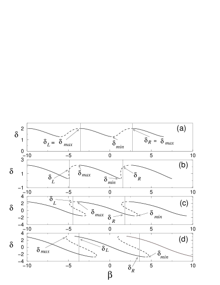
Figure 26: The phase $\delta$ as a function of $\beta$ for various values of $u$ and $F<F_{\uparrow}^{c}(u)$. Also shown in each frame are the values of $\delta_{min}$ and $\delta_{max}$ defined in Eq. (B) and the boundary points $\delta_{R}$ and $\delta_{L}$ of the connected portion of the function $\delta(\beta)$ that is used to evaluate the integrals determining the coherence in each case. The four curves corresponds to the four cases discussed in the text: (a) $u<u_{sv}(F)$, where $\delta(\beta)$ is single-valued. In this case we can choose $\delta_{L}=\delta_{max}$, which requires $\delta_{R}=\delta_{max}$. As $F$ is increased, $\delta_{max}$ grows until $\delta_{max}=\delta_{L}=\pi$ at $F=F_{\uparrow}^{c}$. (b) $u_{sv}(F)<u\leq u_{1}(F)$; (c) $u_{1}(F)<u\leq u_{2}(F)$; and (d) $u>u_{2}(F)$.

For $u>u_{sv}(F)$, the function $\delta(\beta)$ is multivalued. In this case there are multiple possible metastable states $\delta(\beta)$. We can use any one of these to calculate $r(u,F)$ as long as the chosen state satisfies the imaginary part of the self-consistency condition, and lies in the range $[-\pi,\pi]$, but as explained above we choose to focus on the one corresponding to a connected portion of $\delta(\beta)$. As $u$ is increased at fixed $F$, $\delta_{L}(u,F)$ increases and $\delta_{R}(u,F)$ decreases. For hard pinning forces $\delta_{R}$ reaches $\delta_{min}$ before $\delta_{L}$ reaches $\delta_{max}$. It is then convenient to distinguish three regions.

1. $u_{sv}(F)<u\leq u_{1}(F)$, where $u_{1}(F)$ is the value of $u$ where $\delta_{R}=\delta_{min}$. In this region the connected portion includes all of the $\beta_{0}(\delta)$ piece and some of both the $\beta_{-1}(\delta)$ and $\beta_{1}(\delta)$ pieces as shown in Fig. 26(b). The imaginary part of the self consistency condition is then given by

   $$0 = \int_{\delta_{L}}^{\delta_{max}}d\delta\left({d\beta_{-1}\over d\delta}\right)\sin[\delta+\beta_{-1}(\delta)]$$ (79)

   $$+ \int_{\delta_{max}}^{\delta_{min}}d\delta\left({d\beta_{0}\over d\delta}\right)\sin[\delta+\beta_{0}(\delta)]$$

   $$+ \int_{\delta_{min}}^{\delta_{R}}d\delta\left({d\beta_{1}\over d\delta}\right)\sin[\delta+\beta_{1}(\delta)]\;,$$

   with the additional requirement

   $$\beta_{-1}(\delta_{L})+2\pi=\beta_{1}(\delta_{R})\;.$$ (80)

   Once the values of $\delta_{L}(u,F)$ and $\delta_{R}(u,F)$ have been obtained by solving Eqs. (79) and (80), the function $f(u,F)$, is computed using Eq. (70), which now has the explicit form

   $$f(u,F) = \int_{\delta_{L}}^{\delta_{max}}d\delta\left({d\beta_{-1}\over d\delta}\right)\cos[\delta+\beta_{-1}(\delta)]$$ (81)

   $$+ \int_{\delta_{max}}^{\delta_{min}}d\delta\left({d\beta_{0}\over d\delta}\right)\cos[\delta+\beta_{0}(\delta)]$$

   $$+ \int_{\delta_{min}}^{\delta_{R}}d\delta\left({d\beta_{1}\over d\delta}\right)\cos[\delta+\beta_{1}(\delta)]\;.$$

2. $u_{1}(F)<u\leq u_{2}(F)$, where $u_{2}(F)$ is the value of $u$ where $\delta_{L}=\delta_{max}$. In this region the connected portion includes only parts of the $\beta_{0}(\delta)$ and $\beta_{-1}(\delta)$ pieces

   In this region $\delta_{L}>\delta_{max}$, but $\delta_{R}<\delta_{min}$, as shown in Fig. 26(c). The imaginary part of the self consistency condition is then given by

   $$0 = \int_{\delta_{L}}^{\delta_{max}}d\delta\left({d\beta_{-1}\over d\delta}\right)\sin[\delta+\beta_{-1}(\delta)]$$ (82)

   $$+ \int_{\delta_{max}}^{\delta_{R}}d\delta\left({d\beta_{0}\over d\delta}\right)\sin[\delta+\beta_{0}(\delta)]\;,$$

   where

   $$\beta_{-1}(\delta_{L})+2\pi=\beta_{0}(\delta_{R})\;.$$ (83)

   This pair of equations yields $\delta_{L}$ and $\delta_{R}$, which can then be used to calculate $f(u,F)$ as

   $$f(u,F) = \int_{\delta_{L}}^{\delta_{max}}d\delta\left({d\beta_{-1}\over d\delta}\right)\cos[\delta+\beta_{-1}(\delta)]$$ (84)

   $$+ \int_{\delta_{max}}^{\delta_{R}}d\delta\left({d\beta_{0}\over d\delta}\right)\cos[\delta+\beta_{0}(\delta)]\;.$$

3. $u>u_{2}(F)$. In this region the simply connected portion of the $\delta(\beta)$ curve only contains part of the $n=0$ branch, and none of the $n=\pm 1$ branches as shown in Fig. 26(d). The imaginary part of the self consistency condition reads

   $$0 = \int_{\delta_{L}}^{\delta_{R}}d\delta\left({d\beta_{0}\over d\delta}\right)\sin[\delta+\beta_{0}(\delta)]\;,$$ (85)

   with

   $$\beta_{0}(\delta_{L})+2\pi=\beta_{0}(\delta_{R})\;,$$ (86)

   and the function $f(u,F)$ is given by

   $$f(u,F) = \int_{\delta_{L}}^{\delta_{R}}d\delta\left({d\beta_{0}\over d\delta}\right)\cos[\delta+\beta_{0}(\delta)]\;.$$ (87)

As discussed earlier, the depinning force is defined by Eq. (74), i.e. it is given by the value of $F$ where $\delta_{u}=\pi$. For all values of $u<u_{2}$, we can obtain a simple analytical expression for $F_{\uparrow}^{c}$ since in this region $\delta_{u}(u,F_{\uparrow}^{c})=\delta_{max}(u,F_{\uparrow}^{c})=\pi$. Substituting in Eq. (B), we obtain

$$\delta_{max}(u,F_{\uparrow}^{c})=-Y^{-1}(F_{\uparrow}^{c}+u)=\pi\;,$$ (88)

which is easily solved to give

$$F_{\uparrow}^{c}(u)=1-u,\hskip 14.45377ptu\leq u_{2}(F_{\uparrow}^{c})\;.$$ (89)

For $u>u_{2}$, $\delta_{max}$ is outside the connected portion of the curve included in the integration and $\delta_{u}=\delta_{L}$. So threshold is reached when $\delta_{L}=\pi$. In this case it is convenient to directly solve for the depinning threshold by setting $\delta_{L}=\pi$ and $F=F_{\uparrow}^{c}$ in the self-consistency condition, which is given by

$$0=\int_{\delta_{L}=\pi}^{\delta_{R}(u,F_{\uparrow}^{c})}d\delta\left({d\beta_{0}(\delta,u,F_{\uparrow}^{c})\over d\delta}\right)\sin[\delta+\beta_{0}(\delta,u,F_{\uparrow}^{c})]\;,$$ (90)

with

$$\beta_{0}(\delta_{L}=\pi)+2\pi=\beta_{0}\big{(}\delta_{R}(u,F_{\uparrow}^{c})\big{)}\;.$$ (91)

Together these two equations yield $F_{\uparrow}^{c}(u)$. In Fig.(27) we plot $F_{\uparrow}^{c}(u)$ vs $u$ for the hard pinning potential, $Y(x)=-(x+x^{3})/(\pi+\pi^{3})$.

Figure 27: The force $F_{\uparrow}^{c}(u)$, as a function of $u$ for the hard pinning force, $Y(x)=-(x+x^{3})/(\pi+\pi^{3})$. The arrows indicate the values $u_{sv}^{*}$, $u_{1}^{*}$, and $u_{2}^{*}$ separating the four different regions discussed in the text. These values are defined by the relations $u_{sv}(F_{\uparrow}^{c}(u_{sv}^{*}))=u_{sv}^{*}$, $u_{1}(F_{\uparrow}^{c}(u_{1}^{*}))=u_{1}^{*}$ and $u_{2}(F_{\uparrow}^{c}(u_{2}^{*}))=u_{2}^{*}$. The plot becomes nonlinear beyond $u_{2}^{*}$ where the threshold goes from being determined by $\delta_{max}=\pi$ to being determined by $\delta_{L}=\pi$.

The method for obtaining $F_{\uparrow}^{c}(\mu)$ for monotonic soft pinning forces is analogous to that for the hard pinning force, except for one difference. In the case of a monotonic soft pinning force, the value of $\delta_{L}$ reaches $\delta_{max}$ before $\delta_{R}$ reached $\delta_{min}$ (the reverse takes place for monotonic hard pinning forces). This means that $u_{2}<u_{1}$ so that region 1 is now defined by $u_{sv}<u<u_{2}$, region 2 by $u_{2}<u<u_{1}$ and region 3 by $u>u_{1}$. Of course the single valued region remains $u<u_{sv}$. It is not difficult to see that only the expressions for region 2 will differ. In this region the imaginary part of the self consistency condition becomes

$$0 = \int_{\delta_{L}}^{\delta_{min}}d\delta\left({d\beta_{0}\over d\delta}\right)\sin(\delta+\beta_{0}(\delta))$$ (92)

$$+ \int_{\delta_{min}}^{\delta_{R}}d\delta\left({d\beta_{1}\over d\delta}\right)\sin(\delta+\beta_{1}(\delta))\;,$$

which along with

$$\beta_{0}(\delta_{L})+2\pi=\beta_{1}(\delta_{R})$$ (93)

determines $\delta_{L}$ and $\delta_{R}$. The expression for $f(u,F)$ in region 2 is now

$$f(u,F) = \int_{\delta_{L}}^{\delta_{min}}d\delta\left({d\beta_{0}\over d\delta}\right)\cos[\delta+\beta_{0}(\delta)]$$ (94)

$$+ \int_{\delta_{min}}^{\delta_{R}}d\delta\left({d\beta_{1}\over d\delta}\right)\cos[\delta+\beta_{1}(\delta)]\;.$$

B.2 $F_{\uparrow}^{c}$ For Non-Monotonic $Y(\delta)$

The method for obtaining $F_{\uparrow}^{c}(\mu)$ for non-monotonic $Y(\delta)$ is analogous to that outlined for monotonic $F_{\uparrow}^{c}(u)$. Matters are complicated, however, by the existence of additional unstable solutions of the kind discussed for $F=0$ in Appendix A. In principle there is no difference in obtaining $F_{\uparrow}^{c}(\mu)$; one must simply be careful to ensure that only stable solutions are being considered. The differences in the calculation are quite technical and we spare the reader the details.

Appendix C Numerics

To explore the phase diagrams of the mean-field model, we numerically integrated the equations of motion to determine $v$ and $r$ as a function of $F$ and $\mu$. As seen in the main text and earlier appendices, the macroscopic behavior can depend on the preparation of the initial state. For $N$ degrees of freedom $i=1,2,\ldots,N$, the $\beta_{i}$ for most studies were set uniformly, $\beta_{i}=\frac{2\pi}{N}i$. We studied several different initial conditions. One of the most frequently used was to set all $\theta_{i}=\beta_{i}$ at $F=0$, which prepares the system in the incoherent static (IS) state, whenever it is stable. In order to prepare the system in a static coherent state, all phases would be set equal to zero. Coherent moving or static states were also prepared by starting from a high field $F$ with, say, random initial positions $\theta_{i}$. (Incoherent moving states were prepared in some portion of the phase diagram. When preparing incoherent sliding states, we used $M^{2}=N$ degrees of freedom, with $M$ distinct values for $\beta$; the values of $\theta_{i}$ for each $\beta$ value were equally spaced in time based on the periodic single-particle ($r=0$) solution to the equations of motion for the given $\beta$.) Given the initial conditions, we typically computed $v(F)$ and $r(F)$ at fixed $\mu$. This was done by integrating the equations of motion Eq. (3) using the fourth-order Runge-Kutta scheme. The force was raised in small discrete steps: after some amount of time $t_{\rm eq}$ at fixed force, $v$ and $r$ are measured and then $F$ is increased (decreased) some small amount $\delta F$. With this algorithm, the time average of the ramp rate $dF/dt$ is given by $\delta F/t_{\rm eq}$. In some cases, we fixed $F$ and ramped $\mu$ up and down in a similar fashion.

While the ramp rate and system size does affect the depinning force, the force at which $v$ goes from zero to non-zero, we find generically that for ramp rates smaller than $10^{-5}$ and sizes $N$ greater than $256$, we obtain results for both the incoherent and coherent depinning line that are relatively independent of actual ramp rate or system size and agree with analytical calculations. There is agreement even though the coherent depinning curve is analytically obtained using the assumption that $u$ is adiabatically increased. For the simulations, on the other hand, $F$ or $\mu$ is increased (decreased) slowly. Adiabatically ramping $\mu$ is not necessarily equivalent to adiabatically ramping $u$ since the former does not insure that $r$ changes slowly, but we do find the correct coherent depinning line by sitting at a fixed $F$ and ramping up $\mu$.

The analytical analysis in Secs. V and VI provides us with the depinning line as approached from the pinned phase, but it does not give us insight into the nature of the depinning transition. For example, there could be hysteresis in $v(F)$ or $r(F)$ for cyclical histories in the force, for sufficiently large system sizes and arbitrarily small ramp rates. Hysteresis in the order parameters implies that the depinning transition is discontinuous. If there is hysteresis in $v(F)$, then the depinning line as approached from the moving phase must be different from the depinning line computed in Secs. VI and V. To numerically search for hysteresis, we prepare the system in a coherent moving state and lower the force until the system stops. If this repinning line is different from the analytical depinning result, hysteresis between the static (IS or CS) and moving phases is present and there is a region where the two phases coexist.

For every potential investigated, we find that there is a range of $0<\mu<\mu_{e}$ where there is a coexistence of the moving and stationary solutions. In general, there is hysteresis between coherent moving (CM) and incoherent static (IS) phases. For the piecewise linear pinning force, the hysteresis extends into the coherent pinned CS region. In other words, the coherence $r$ jumps from one finite value to another at the depinning transition and there is hysteresis in both $r$ and $v$ ($F_{\downarrow}\neq F^{c}_{\uparrow}$). The numerical evidence for this is shown in Fig. 28, which shows the area of the hysteresis loop, $\int_{0}^{\infty}dF\,\left[v^{\downarrow}(F)-v^{\uparrow}(F)\right]$, where $v^{\downarrow}(F)$ and $v^{\uparrow}(F)$ are the histories of $v(F)$ for ramping the field down or up, respectively. The amount of hysteresis, as measured by this quantity, is independent of system size and $dF/dt$, which suggests that the simulations are close the adiabatic and infinite-volume limit. There is a jump down in the area of the hysteresis loop when $\mu$ exceeds $\mu_{u}$, but the area is still non-zero for $\mu>\mu_{u}$.

Figure 28: (a) Area of the hysteresis loop in $v(F)$ as F is cycled from large values to zero and then back up again near $\mu_{e}\approx 0.75$ for the scalloped potential. Different system sizes and ramp rates $dF/dt$ are shown. Plot (b) is just a blowup of (a) very near $\mu_{e}$.

For the hard potential, with the history described above, $r$ jumps to zero when the system becomes pinned. When the drive is increased back up again, the system depins at a different $F_{\uparrow}^{i}$ when $\mu<\mu_{e}$. However, we do not observe hysteresis between the CM and CS phases. In fact, the hysteresis when ramping $F$ vanishes suddenly at $\mu=\mu_{e}$. See Fig. 29. This is because the slope of the coherent depinning line starts to increase rapidly at $(\mu_{e},F_{e})$ and eventually becomes infinite before curling over to possible hysteresis. Above the point at which the slope becomes infinite, the analytic calculations suggest that coherent depinning can be observed by increasing $\mu$ at fixed $F$. This was verified numerically. For the soft-potential cases tested we did not observe hysteresis between the CS and CM phases. Hysteresis is only observed between the IS and CM phases.

Figure 29: Area of the hysteresis loop in $v(F)$ near $\mu_{e}$ for the hard case, where $\mu_{e}$ is the intersection of $F_{\uparrow}^{i}$ and $F_{\uparrow}^{c}$. Different system sizes and ramp rates are shown.

Appendix D Stability of the IM Phase

In this section we investigate the existence of a stable incoherent sliding (IM) phase. We note that the velocity of a single degree of freedom is always a periodic function of time. To obtain a constant steady state velocity for a collection of incoherent degrees of freedom, we assume that at some initial time $t_{i}$ the $i$-th degree of freedom is at the minimum of its own potential well, which in turn is randomly shifted by $\beta$, and perform an average over the random starting times $t_{i}$. These are chosen to be random variables uniformly distributed on the interval $[0,P]$, with $P$ being the period, that is the time over which the phases advance by $2\pi$. This procedure guarantees that we sample uniformly all possible incoherent moving states such that the system reaches a steady state.

Proceeding as in the study of the incoherent static state, we assume that the IM phase exists and study its stability. The self-consistency condition that must be satisfied by the mean field solution is given by

$$r(t)e^{i\psi(t)}=\int_{P}\frac{dt_{i}}{P}\int^{\pi}_{-\pi}\frac{d\beta}{2\pi}e^{i\theta(t-t_{i},\beta)}\;,$$ (95)

where the phase $\theta(t-t_{i},\beta)$ is the phase at a time $t>t_{i}$ obtained by solving the equation of motion. In eq. (95), both the coherence $r$ and the mean phase $\psi$ are functions of time. As in the static stability analysis, we let $\delta(t-t_{i},\beta)=\theta(t-t_{i},\beta)-\beta$. We then perturb the IM state at the time $t=0$, with a perturbation of the form

$$\delta_{p}(-t_{i},\beta)=\delta_{0}(-t_{i})-\epsilon\sin\left(\beta+\delta_{0}(-t_{i})\right)\;,$$ (96)

with $\epsilon<<1$. After inserting this in Eq. (95), we evaluate the right hand side at $t=0$ to $\mathcal{O}(\epsilon)$, obtaining $r(t=0)=\epsilon/2$ and $\psi(t=0)=0$. We then use this to compute $\dot{r}(0)$ to linear order, with the result

$$\dot{r}(0)=\frac{\epsilon}{2}\bigg{[}\frac{\mu}{2}+\int_{P}\frac{dt_{i}}{P}Y^{\prime}(\delta_{0}(-t_{i}))\bigg{]}\;.$$ (97)

If $r(t)$ is monotonic in time, then its stability is entirely determined by the sign of $\dot{r}(0)$. We would then conclude that there is a critical value $\mu_{c}(F)$ of the coupling strength below which the IM phase is stable, with

$$\mu_{c}(F)=-\frac{2}{P}\int_{P}\frac{dt_{i}}{P}Y^{\prime}(\delta_{0}(-t_{i}))\;.$$ (98)

With a change of variable from $t_{i}$ to $\delta_{0}$ (using the equation of motion), one finds that $\mu_{c}=0$ for all $F>F_{\rm sp}$ for any continuous pinning force (since $Y(\pi)=0$). For discontinuous pinning forces, however, we can evaluate the integral in Eq. (98) by splitting the integral in a contribution from the smoothly varying part of $Y^{\prime}(\delta_{0})$ on the interval $[-\pi,\pi)$ and a jump at $\delta_{0}=\pi$. This gives

$$\mu_{c}(F)=-\frac{2}{P}\bigg{[}\ln(\frac{F+|Y(\pi)|}{F-|Y(\pi)|})-2\frac{Y(\pi)}{F+|Y(-\pi)|}\bigg{]}\;,$$ (99)

where $P$ is a function of $F$. For the piecewise linear force, one can evaluate $P$ and find $\mu_{c}(F)>0$ for some $F>F_{\rm sp}$. The critical value of $\mu_{c}(F)$ is given by

$$\mu_{c}(F)=\mu_{u}\bigg{[}1-\frac{2}{\ln(\frac{F+a\pi}{F-a\pi})(F+a\pi)}\bigg{]}.$$ (100)

In the limit of large $F$, $\mu_{c}$ approaches zero. As $F$ approaches $F_{\rm sp}$, on the other hand, $\mu_{c}=\mu_{u}$. In other words, the IM stability curve abruptly ends at $(\mu_{u},F_{\rm sp})$ as there can be no IM phase for any $F$ less than $F_{\rm sp}$. A transition from an incoherent to a coherent moving phase was indeed obtained theoretically by Vinokur and Nattermann NV97 in a model of for layered charge density waves and also observed by Olson et al. Olson01 in numerical simulations of layered superconductors. For strong disorder, these authors found a transition as the drive is increased from a $2D$ state of decoupled moving layers to a $3D$ state where the moving layers become coupled. Our short time results suggest that a similar transition may occur in the isotropic system studied here. However, our numerical studies indicate that this transition may be an artifact of the short time analysis. When testing the stability of a system prepared in the IM phase numerically, we find that $r(t)$ is generally not a monotonic function of time. Furthermore, a perturbation of strength $\epsilon$ always destabilizes the IM phase in the limit of large system size, unless the strength of the perturbation is made to decrease with system size. Finally, we verified that the IM phase remains unstable if the somewhat artificial average over the starting times $t_{i}$ is replaced by an average over a narrow distribution of pinning strengths. Given these numerical findings, we conclude that the IM phase is typically unstable in the isotropic mean field model studied here, although of course we cannot rule out that the system could be prepared in such a state by some special initial condition.

References

- (1) D. S. Fisher, Phys. Rep. 301, 113 (1998).
- (2) D. S. Fisher, Phys. Rev. B 31, 1396 (1985).
- (3) O. Narayan and D. S. Fisher, Phys. Rev. B 46, 11520 (1992).
- (4) A. A. Middleton, Phys. Rev. Lett. 68, 670 (1992).
- (5) D. Ertas and M. Kardar, Phys. Rev. B 53, 3520 (1996).
- (6) P. Le Doussal, K.J. Wiese, and P. Chauve, Phys. Rev. B 66, 174201 (2002).
- (7) T. Nattermann, S. Stepanow, L.-H. Tang, and H. Leschhorn, J. Phys. II France, 2, 1483 (1992).
- (8) S. N. Coppersmith and P. B. Littlewood, Phys. Rev. Lett. 57, 1927 (1986) .
- (9) S. N. Coppersmith and P. B. Littlewood, Phys. Rev. B 36, 311 (1987).
- (10) A. A. Middleton and D. S. Fisher, Phys. Rev. Lett. 66, 92 (1991).
- (11) A. A. Middleton and D. S. Fisher, Phys. Rev. B 47, 3530 (1993).
- (12) C. R. Myers and J. P. Sethna, Phys. Rev. B 47, 11171 (1993).
- (13) A. Rosso, A. K. Hartmann, and W. Krauth, Phys. Rev. E 67, 021602 (2003).
- (14) A. E. Koshelev and V. M. Vinokur, Phys. Rev. Lett. 73, 3580 (1994).
- (15) T. Giamarchi and P. Le Doussal, Phys. Rev. Lett. 76, 3408 (1996).
- (16) L. Balents, M.C. Marchetti, and L. Radzihovsky, Phys. Rev. B 57, 7705 (1998).
- (17) K. Moon, R. T. Scalettar, and G.T. Zimanyi, Phys. Rev. Lett. 77, 2778 (1996).
- (18) F. Pardo, F. de la Cruz, P.L. Gammel, E. Bucher, and D.J. Bishop, Nature 396, 348, (1998).
- (19) “Coexistence” here, within mean field theory, refers to multistability of the solutions to the equations of motion. As is typical in mean field theory, there is no natural notion of an interface in these calculations, so it is not possible for both of these phases to exist simultaneously in the same mean-field sample, though the question of an interface is open in finite dimensions.
- (20) L. Balents and M. P. A. Fisher, Phys. Rev. Lett. 75, 4270 (1995).
- (21) A. Maeda, T. Fukuyama, and S. Tanaka, Solid. State Comm. 55, 951 (1985).
- (22) A. Maeda, N. Notomi, and K. Uchinokura, Phys. Rev. B 42, 3290 (1990).
- (23) R. E. Thorne, K. Cicak, K. O’Neill and S. G. Lemay, J. Phys. IV 12, 291 (2002); and references therein.
- (24) This can also result from inertial effects.
- (25) S.H. Strogatz, C.M. Marcus, R.M. Westervelt, and R.E. Mirollo, Phys. Rev. Lett. 61, 2380 (1988); Physics D 36, 23 (1989).
- (26) J. Levy, M. S. Sherwin, F. F. Abraham, and K. Wiesenfeld, Phys. Rev. Lett. 68, 2968 (1992).
- (27) A. Montakhab, J. M. Carlson and J. Levy, Phys. Rev. B 50, 11227 (1994).
- (28) V. M. Vinokur and T. Nattermann, Phys. Rev. Lett. 79, 3471 (1997).
- (29) M. C. Marchetti, A. A. Middleton and T. Prellberg, Phys. Rev. Lett. 85, 1104 (2000).
- (30) M. C. Marchetti and K. A. Dahmen, Phys. Rev. B 66, 214201 (2002).
- (31) J. M. Schwarz and D.S. Fisher, Phys. Rev. Lett. 87, 96107 (2001).
- (32) J. M. Schwarz and D. S. Fisher, Phys. Rev. E 67, 021603 (2003).
- (33) M. C. Marchetti, A. A. Middleton, K. Saunders, and J. M. Schwarz, Phys. Rev. Lett. 91, 107002 (2003).
- (34) G. Grüner, Rev. Mod. Phys. 60, 1129 (1998).
- (35) R. E. Thorne, Physics Today 49, 42 (1996).
- (36) S. N. Coppersmith, Phys. Rev. Lett. 65, 1044 (1990); Phys. Rev. B 44, 2887 (1991).
- (37) S. N. Coppersmith and A. J. Millis, Phys. Rev. B 44, 7799 (1991).
- (38) C. R. Myers, in Structured adaptive mesh refinement (SAMR) grid methods - The IMA Volumes in Mathematics and Its Applications, 117 (Springer-Verlag, 1999).
- (39) M. Karttunen, M. Haatja, K. R. Elder, and M. Grant, Phys. Rev. Lett. 83, 3518 (1999).
- (40) R. P. Hall, M. F. Hundley, and A. Zettl, Phys. Rev. B 38, 13002 (1988).
- (41) T. L. Adelman, J. McCarten, M. P. Maher, D. A. DiCarlo, and R. E. Thorne, Phys. Rev. B 47, 4033 (1993).
- (42) M. P. Maher, T. L. Adelman, J. McCarten, and D. A. DiCarlo, Phys. Rev. B 43, 9968 (1991).
- (43) S. G. Lemay, M. C. de Lind van Wijngaarden, T. L. Adelman, and R. E. Thorne, Phys. Rev. B 57, 12781 (1998).
- (44) H. J. Jensen, A. Brass, and A. J. Berlinsky, Phys. Rev. Lett. 60, 1676 (1988).
- (45) H. J. Jensen, A. Brass, Y. Brechet, and A. J. Berlinsky, Phys. Rev. B 38, 9235 (1988).
- (46) F. Nori, Science 271, 1373 (1996).
- (47) C. J. Olson, C. Reichhardt, and F. Nori, Phys. Rev. Lett. 81, 3757 (1998).
- (48) N. Gronbech-Jensen, A. R. Bishop, and D. Dominguez, Phys. Rev. Lett. 76, 2985 (1996).
- (49) M. C. Faleski, M. C. Marchetti, and A. A. Middleton, Phys. Rev. B 54, 12427 (1996).
- (50) M. Marchevsky, J. Aarts, P. H. Kes, and M. V. Indebom, Phys. Rev. Lett. 78, 531 (1997).
- (51) A. Tonomura, Micron 30, 479 (1999).
- (52) A. M. Troyanovski, J. Aarts, and P. H. Kes, Nature 399, 665 (1999).
- (53) A. M. Troyanovski, M. van Hecke, N. Saha, J. Aarts, and P. H. Kes, Phys. Rev. Lett. 89, 147006 (2002).
- (54) S. Bhattacharya and M.J. Higgins, Phys. Rev. Lett. 70, 2617 (1993); S. Bhattacharya and M.J. Higgins, Phys. Rev. B 52, 64 (1995); M.J. Higgins and S. Bhattacharya, Physica C 257, 232 (1996).
- (55) M. C. Hellerqvist, D. Ephron, W. R. White, M. R. Beasly, and A. Kapitulnik, Phys. Rev. Lett. 76, 4022 (1996); M. C. Hellerqvist and A. Kapitulnik, Phys. Rev. B 56, 5521 (1997).
- (56) A. Maeda, T. Tsuboi, R. Abiru, Y. Togawa, H. Kitano, K. Iwaya, and T. Hanaguri, Phys. Rev. B 65, 054506 (2002).
- (57) Y. Paltiel, E. Zeldov, Y. N. Myasoedov, K. Shtrikman, S. Bhattacharya, M. J. Higgins, Z. L. Xiao, E. Andrei, P. L. Gammel, and D. J. Bishop, Nature 403, 398 (2000).
- (58) Y. Paltiel, Y. Myasoedov, E. Zeldov, G. Jung, M.L. Rappaport, D. E. Feldman, M.J. Higgins, and S. Bhattacharya, Phys. Rev. B 66, 60503 (2002).
- (59) M. Marchevsky, M. J. Higgins, and S. Bhattacharya, Phys. Rev. Lett. 88, 87002 (2002).
- (60) L. P. Gor’kov, Pis’ma Zh. Eksp. Teor. Fiz. 38, 76 (1983) [JETP—Lett. 38, 87 (1983)].
- (61) N. P. Ong and K. Maki, Phys. Rev. B 32, 6582 (1985).
- (62) M. Inui, R. P. Hall, S. Doniach, and A. Zettl, Phys. Rev. B 38, 13047 (1988).
- (63) A. A. Middleton, Ph.D. thesis, Princeton University, 1990.
- (64) Y. Kuramoto, Chemical Oscillations, Waves, and Turbulence (Springer, Berlin, 1984).
- (65) H. Fukuyama and P. A. Lee, Phys. Rev. B 17, 535 (1978); P. A. Lee and T. M. Rice, Phys. Rev. B 19, 3970 (1979).
- (66) In the case it is possible to solve for . This is demonstrated in Strogatz, .
- (67) The astute reader will question the suitability of choosing to evaluate in an adiabatically increasing scenario. This is because perturbation theory has already shown that for “soft” and piecewise linear pinning forces it is not possible to adiabatically increase due to the existence of a jump in . Numerical analysis shows however that the metastable states accessed through adiabatically increasing are the same as those that would be accessed were it possible to adiabatically increase .
- (68) Note that there are two functions which represents the dependence of the coherent depinning threshold on and which represents the dependence of the coherent depinning threshold on . These two functions are distinguished by their arguments. To avoid confusion it may be preferable to denote the latter as , then can be written as . However, since this leads to cumbersome nomenclature, we do not use it here.
- (69) C. J. Olson, C. Reichhardt and V.M. Vinokur, Phys. Rev. B 64, 140502 (2001).
- (70) A. Pertsinidis and X. S. Ling, Bull. Am. Phys. Soc. 48 (2001).
- (71) C. Reichhardt and C. J. Olson, Phys. Rev. Lett. 89, 078301 (2002).