Local quantum phase transition in the pseudogap Anderson model: scales, scaling and quantum critical dynamics

Abstract

The pseudogap Anderson impurity model provides a paradigm for understanding local quantum phase transitions, in this case between generalised fermi liquid and degenerate local moment phases. Here we develop a non-perturbative local moment approach to the generic asymmetric model, encompassing all energy scales and interaction strengths and leading thereby to a rich description of the problem. We investigate in particular underlying phase boundaries, the critical behaviour of relevant low-energy scales, and single-particle dynamics embodied in the local spectrum $D(\omega)$. Particular attention is given to the resultant universal scaling behaviour of dynamics close to the transition in both the GFL and LM phases, the scale-free physics characteristic of the quantum critical point itself, and the relation between the two.

1 Introduction

The essential physics of a single magnetic impurity coupled to a fermionic host is embodied at its simplest in the Anderson impurity model (AIM) [1]: a correlated, non-degenerate impurity with local interaction $U$, hybridizing to a non-interacting host band with density of states $\rho_{\mbox{\scriptsize{host}}}(\omega)$ (for a comprehensive review see [2]). Yet its simplicity is nominal — even for the conventional case of a metallic host, the basic model for understanding magnetic impurities in metals [1,2] and highly topical again in the context of quantum dots for example [3,4], or surface atoms probed by scanning tunneling microscopy (STM) [5]. Here the essential strong coupling (large-$U$) behaviour is that of the Kondo effect, characterised by a single low-energy Kondo scale $\omega_{\mbox{\scriptsize{K}}}$, manifest vividly in the Kondo resonance in the local single-particle spectrum $D(\omega)$, and rendered no less subtle for being by now quite well understood.

There is however one sense in which the metallic AIM is ‘simple’: it lacks a non-trivial quantum phase transition. The impurity spin is quenched ubiquitously by coupling to the low-energy degrees of freedom of the metallic host, the system is a Fermi liquid for all interaction strengths $U$ and the Kondo scale, while exponentially small in strong coupling, never quite vanishes.

That situation changes markedly if the host contains instead a pseudogap in the vicinity of the Fermi level [6] ($\omega=0$), namely $\rho_{\mbox{\scriptsize{host}}}(\omega)\propto|\omega|^{r}$ with $r>0$ (and $r=0$ corresponding to the normal metallic AIM). This pseudogap Anderson impurity model (PAIM) has been studied extensively in recent years [6-20], particularly for large-$U$ where the low-energy subspace maps onto that of the associated Kondo model, and from which work much progress and insight has accrued. The resultant depletion of host states around the Fermi level leads in general to the occurrence [6-20] of a quantum phase transition at a finite, $r$-dependent $U_{\mbox{\scriptsize{c}}}$. Above the quantum critical point (QCP) a degenerate local moment (LM) phase arises, with a residual, unquenched impurity spin. For $U<U_{\mbox{\scriptsize{c}}}$ by contrast, and perturbatively connected to the non-interacting limit ($U=0$), resides a ‘strong coupling’ or generalised Fermi liquid (GFL) phase in which the impurity spin is locally quenched and a Kondo effect manifest, reflected in a low-energy Kondo scale $\omega_{\mbox{\scriptsize{K}}}$. In the vicinity of the transition each phase is in fact characterised by a low-energy scale [17-20], here denoted generically by $\omega_{*}$; corresponding to the Kondo scale $\omega_{*}\equiv\omega_{\mbox{\scriptsize{K}}}$ for the GFL phase and its counterpart $\omega_{*}\equiv\omega_{\mbox{\scriptsize{L}}}$ [20] for the LM phase. Most importantly, and symptomatic of the underlying transition, the $\omega_{*}$’s vanish as the QCP is approached.

Although the PAIM serves in general as a paradigm for understanding local (boundary) quantum phase transitions [21], many examples of specific systems with a power-law density of states have also been discussed. These include various zero-gap semiconductors [22], one-dimensional interacting systems [23], and the important problem of impurity moments in $d$-wave superconductors [17,18], notably $Zn$- and $Li$- doped cuprate materials. Likewise it has recently been shown [19] that the pseudogap Kondo model exhibits critical local moment fluctuations, and an associated destruction of the Kondo effect, very similar to those present at the local QCP of the Kondo lattice [24] that has been argued to explain the behaviour of heavy fermion metals such as CeCu_6-xAu_x.

While great progress has been made in understanding the PAIM [6-20], much nevertheless remains to be understood; particularly regarding the quantum critical behaviour of dynamical properties close to and on either side of the transition, and precisely at the QCP itself. Since the low-energy scale $\omega_{*}$ is arbitrarily small (but non-zero) sufficiently close to the transition, the frequency ($\omega$) dependence of dynamics should scale in terms of it — i.e. exhibit universal scaling as a function of $\omega/\omega_{*}$ — with resultant scaling behaviour that will depend on the particular phase considered, GFL or LM. What precisely is that behaviour for the selected dynamical property? And how from it does (or can) one understand the scale-free physics characteristic of the QCP itself, where $\omega_{*}=0$ identically? These are tough issues, especially from an analytical perspective, and some key aspects of which have recently been uncovered via numerical renormalization group (NRG) calculations [16,18,19], the local moment approach [15,16,20] and, for the multichannel pseudogap Kondo model, a dynamic large-$N$ approach [17]. Single-particle spectra embodied in the impurity $D(\omega)$ provide an obvious example of dynamics [12, 14-20]; and an important one given e.g. the direct manifestation in the GFL phase of low-energy Kondo physics embodied in the Kondo resonance, as well as their more general relevance to STM and related experimental techniques.

In this paper we develop a local moment approach (LMA) [25-30,15,20] to the PAIM at $T=0$, for the general case of the particle-hole asymmetric model (noting that the corresponding Kondo model thus contains both exchange and potential scattering). Single-particle dynamics form a central focus of the theory albeit, importantly, that its intrinsic formulation also enables phase boundaries between the GFL and LM phases to be determined, as well as the critical behaviour of associated low-energy scales [15,20]. Although developed originally to describe metallic Anderson impurity models, at $T=0$ [25-27], finite temperatures [28] and magnetic fields [29], the approach is quite general; readily extended for example to encompass lattice-based models within the framework of dynamical mean-field theory, such as the periodic Anderson lattice model [30]. It has also been applied previously to and has led to a number of new predictions for, the symmetric limit of the PAIM [15,20]; rather successfully, as judged by subsequent comparison to NRG calculations [16]. The asymmetric PAIM considered here is however another matter: the symmetric model, recovered though it is as a particular limit of the present work, has long been argued [13,17,18] to be a somewhat special case, in some sense divorced from generic asymmetric behaviour (although our own caveats on the matter will become clear in due course).

The LMA, while certainly approximate, is also well suited to the present problem. Its intrinsically non-perturbative nature enables it to handle strong electron correlations and the attendant, central low-energy scales; while at the same time permitting access to dynamics on all energy scales, whether it be on the $\omega_{*}$ scales relevant to universal scaling behaviour, or scales on the order of $\omega\sim U$ relevant to the high-energy Hubbard satellites. Importantly too, and in contrast to difficulties inherent to a number of other potential theoretical approaches, the method handles both the GFL and LM phases on an essentially equal footing (the LM phase, for example, is certainly not a trivially decoupled/isolated spin).

The paper is organised as follows. After the requisite background, we consider in §2.1 an obvious question: since the GFL phase is pertubatively connected to the non-interacting limit, satisfying as such the Luttinger theorem [31], what is the analogue of the resultant Friedel sum rule? That is entirely familiar for the conventional metallic AIM ($r=0$) [2,32], and its counterpart for the PAIM plays a central role in the present work. In §3 another important issue is considered: what can be deduced on general, minimalist grounds about the behaviour of the scaling spectra close to the quantum phase transition; in both the GFL and LM phases and at the QCP itself? Such considerations are revealing, and dictate constraints to be met by any credible approximate theory. They show moreoever that a variety of low-energy scales in addition to $\omega_{*}$ enter the scaling behaviour of dynamics — the quasiparticle weight $Z$ and renormalised level $\epsilon_{\mbox{\scriptsize{i}}}^{*}$ for the GFL phase, together with the latter’s spin-dependent counterparts for the LM phase. Each vanishes as the transition is approached, with distinct but related critical exponents; but nonetheless enter dynamics in such a way that universal scaling remains determined solely by the key low-energy scale $\omega_{*}$.

The LMA itself is developed in §4, focusing on the notion of symmetry restoration that is central to the approach [15,20,25-30], together with what likewise proves important in dealing with the asymmetric PAIM, namely self-consistent satisfaction of the Friedel sum rule/Luttinger theorem. Results arising from the approach are presented in §s 5-7, beginning with the critical behaviour of relevant low-energy scales (§5.1) and a determination of representative phase diagrams for the problem (§5.2). Single-particle dynamics are considered in §6, on all energy scales whether universal or non-universal; but with a dominant focus on scaling spectra in the GFL and LM phases — on all $\omega/\omega_{*}$ scales — as well as the scale-free dynamics arising at the QCP. Finally, we consider in §7 the regime of small $r\ll 1$, obtaining explicit analytic results for the critical behaviour of low-energy scales, resultant phase boundaries and single-particle scaling spectra. The paper concludes with a brief summary/outlook.

2 Background

With the Fermi level taken as the energy origin, the Hamiltonian for the spin-$\frac{1}{2}$ AIM [1,2] is given by

$$\ \ \ \ \ \hat{H}=\sum_{\bi{k},\sigma}\epsilon_{\bi{k}}\hat{n}_{\bi{k}\sigma}+\sum_{\sigma}(\epsilon_{\mbox{\scriptsize{i}}}+\mbox{$\frac{1}{2}$}U\hat{n}_{\mbox{\scriptsize{i}}-\sigma})\hat{n}_{\mbox{\scriptsize{i}}\sigma}+\sum_{\bi{k},\sigma}V_{\mbox{\scriptsize{i}}\bi{k}}(c^{\dagger}_{\mbox{\scriptsize{i}}\sigma}c_{\bi{k}\sigma}+c^{\dagger}_{\bi{k}\sigma}c_{\mbox{\scriptsize{i}}\sigma}).$$ (2.1)

The first term describes the non-interacting host with density of states $\rho_{\mbox{\scriptsize{host}}}(\omega)=\sum_{\bi{k}}\delta(\omega-\epsilon_{\bi{k}})$, while the second refers to the correlated impurity with bare site-energy $\epsilon_{\mbox{\scriptsize{i}}}$ and on-site interaction $U$. The third term is the one-electron host-impurity coupling embodied in $V_{\mbox{\scriptsize{i}}\bi{k}}$, taken for convenience as $V_{\mbox{\scriptsize{i}}\bi{k}}=V$ (although that is not required). The particle-hole asymmetry of the model is specified by the asymmetry parameter [1,27]

$$\eta=1+\frac{2\epsilon_{\mbox{\scriptsize{i}}}}{U}$$ (2.2)

such that $\eta=0$ corresponds to the particle-hole symmetric case, where $\epsilon_{i}=-\frac{U}{2}$ and the impurity charge $n=\sum_{\sigma}\langle\hat{n}_{\mbox{\scriptsize{i}}\sigma}\rangle=1$ for all $U$. In strong coupling, where the relevant low-energy sector of the AIM maps under a Schrieffer-Wolff transformation onto a Kondo model containing both exchange ($J$) and potential ($K$) scattering contributions [2], the asymmetry $\eta$ is equivalently the ratio of the potential/exchange scattering strengths: $\eta\equiv 1-2|\epsilon_{\mbox{\scriptsize{i}}}|/U=K/J$ (see e.g. [27]).

We focus here on the impurity Green function $G(\omega)(\leftrightarrow G(t)=-\mbox{i}\langle\hat{T}(c_{\mbox{\scriptsize{i}}\sigma}(t)c^{\dagger}_{\mbox{\scriptsize{i}}\sigma})\rangle)$, and hence the local spectrum $D(\omega)=-\frac{1}{\pi}\mbox{sgn}(\omega)\mbox{Im}G(\omega)$. In addition to intrinsic interest in single-particle dynamics per se, this also provides a direct route to both the location of phase boundaries between the GFL and LM states [15] and the critical behaviour of associated low-energy scales, as will be shown in §s 4,5.

$G(\omega)$ is conventionally expressed as

$$G(\omega)=[\omega^{+}-\epsilon_{\mbox{\scriptsize{i}}}-\Delta(\omega)-\Sigma(\omega)]^{-1}$$ (2.3)

with $\omega^{+}=\omega+\mbox{i}0^{+}\mbox{sgn}(\omega)$ and $\Sigma(\omega)=\Sigma^{\mbox{\scriptsize{R}}}(\omega)-\mbox{i}\mbox{sgn}(\omega)\Sigma^{\mbox{\scriptsize{I}}}(\omega)$ the usual single self-energy; the corresponding non-interacting Green function is denoted by $g(\omega)$. All effects of host-impurity coupling at one-electron level are embodied in the hybridization function $\Delta(\omega)=\sum_{\bi{k}}V_{\mbox{\scriptsize{i}}\bi{k}}^{2}[\omega^{+}-\epsilon_{\bi{k}}]^{-1}$ ($=\Delta_{\mbox{\scriptsize{R}}}-\mbox{i}\mbox{sgn}(\omega)\Delta_{\mbox{\scriptsize{I}}}(\omega)$). For the PAIM considered, $\Delta_{\mbox{\scriptsize{I}}}(\omega)=\pi V^{2}\rho_{\mbox{\scriptsize{host}}}(\omega)$ is given explicitly by $\Delta_{\mbox{\scriptsize{I}}}(\omega)=\Delta_{0}(|\omega|/\Delta_{0})^{r}\theta(D-|\omega|)$ with $\Delta_{0}$ the hybridization strength and $D$ the bandwidth ($\theta(x)$ is the unit step function). That this form is naturally simplified is of course immaterial to the relevant low-energy physics of the problem in the scaling regime of primary interest. We take $\Delta_{0}\equiv 1$ as the basic energy unit in this paper, i.e.

$$\Delta_{\mbox{\scriptsize{I}}}(\omega)=|\omega|^{r}\theta(D-|\omega|)$$ (2.4)

with $r>0$ for the pseudogap AIM (and the limit $r=0$ corresponding to the normal metallic model). The real part $\Delta_{\mbox{\scriptsize{R}}}(\omega)$ follows from Hilbert transformation and, for later reference, has the low-$\omega$ behaviour (for all $r\geq 0$)

$$\Delta_{\mbox{\scriptsize{R}}}(\omega)=-\mbox{sgn}(\omega)\left\{\beta(r)|\omega|^{r}+\frac{2D^{r}}{\pi(r-1)}\frac{|\omega|}{D}+\cal{O}\rm\left[\left(\frac{|\omega|}{D}\right)^{3}\right]\right\}$$ (2.5)

with $\beta(r)=\mbox{tan}(\frac{\pi}{2}r)$ used throughout. Notice from this that the wide-band limit $D\rightarrow\infty$, so frequently employed for the metallic AIM (see eg [2]), can be taken for $r<1$, whereupon $\Delta_{\mbox{\scriptsize{R}}}(\omega)=-\mbox{sgn}(\omega)\beta(r)|\omega|^{r}$ for all $\omega$. We consider $0<r<1$ in this paper, which range is assumed unless stated to the contrary; and for that reason will employ the wide-band limit. This is simply a matter of convenience, is again irrelevant to the key low-energy behaviour of the system and can be relaxed trivially.

The impurity charge $n$ is of course related to the local spectrum by $n=2\int^{0}_{-\infty}\mbox{d}\omega\ D(\omega)$. The ‘excess’ charge $n_{\mbox{\scriptsize{imp}}}$ will also prove important to the present work, for reasons given in §2.1. This is defined as the change in the number of electrons of the entire system due to addition of the impurity to the host, and is given generally by

$$n_{\mbox{\scriptsize{imp}}}=2\int^{0}_{-\infty}\mbox{d}\omega\ \Delta\rho(\omega).$$ (2.6)

Here $\Delta\rho(\omega)$ ($=\rho(\omega)-\rho_{\mbox{\scriptsize{host}}}(\omega)$) is the excess density of states, itself given by (see e.g.  [2])

$$\Delta\rho(\omega)=-\frac{1}{\pi}\mbox{sgn}(\omega)\mbox{Im}\left\{G(\omega)\left[1-\frac{\partial\Delta(\omega)}{\partial\omega}\right]\right\}$$ (2.7)

such that $n_{\mbox{\scriptsize{imp}}}$ is related to $n$ by

$$n_{\mbox{\scriptsize{imp}}}=n-\frac{2}{\pi}\mbox{Im}\int^{0}_{-\infty}\mbox{d}\omega\ G(\omega)\frac{\partial\Delta(\omega)}{\partial\omega}.$$ (2.8)

From the above, for specified gap index $r$, the PAIM is characterised by any two of the ‘bare’ parameters $U$, $\epsilon_{\mbox{\scriptsize{i}}}$ and $\eta=1+2\epsilon_{\mbox{\scriptsize{i}}}/U$ (together if appropriate with the bandwidth $D$). In practice, as now explained, we choose to consider $\eta$ and one or other of $U$ and $\epsilon_{\mbox{\scriptsize{i}}}$ as the basic parameters. For the $r=0$ metallic AIM we have recently considered [26,27] the scaling behaviour of $D(\omega)$ arising in the strong coupling Kondo regime, where $\epsilon_{\mbox{\scriptsize{i}}}<0$ such that $|\epsilon_{\mbox{\scriptsize{i}}}|\gg 1$ and $U-|\epsilon_{\mbox{\scriptsize{i}}}|\gg 1$. Here the Kondo scale $\omega_{\mbox{\scriptsize{K}}}$ is exponentially small. For fixed asymmetry $\eta$ [27], $D(\omega)$ then exhibits scaling in terms of $\tilde{\omega}=\omega/\omega_{\mbox{\scriptsize{K}}}$. That is, on fixing $\eta=1-2|\epsilon_{\mbox{\scriptsize{i}}}|/U$ and progressively increasing the interaction $U$, $D(\omega)$ is universally dependent on $\tilde{\omega}=\omega/\omega_{\mbox{\scriptsize{K}}}$ alone, and otherwise independent of the bare model parameters (which themselves determine the Kondo scale). The important point here is that this arises for fixed asymmetry $\eta\equiv K/J$ (and in this case only for fixed $\eta$, i.e. universal scaling does not arise upon increasing $U$ for fixed $|\epsilon_{\mbox{\scriptsize{i}}}|\gg 1$ [27]). In consequence, a family of scaling spectra arises, one for each asymmetry $\eta$. This is not widely appreciated (although in the related context of d.c. transport it was understood early by Wilson [33]), but that it must arise is nearly obvious. For if the scaling spectra for the generic asymmetric AIM were $\eta$-independent, they would coincide with that for the p-h symmetric model $\eta=0$ ($=K/J$) and as such be strictly symmetric in $\omega$ about the Fermi level $\omega=0$; the implausibility of which is at least intuitive.

For the pseudogap model considered here, the quantum phase transition between GFL and LM phases is naturally characterised by a low-energy scale $\omega_{*}$ — the Kondo scale $\omega_{\mbox{\scriptsize{K}}}$ for the GFL phase and its counterpart $\omega_{\mbox{\scriptsize{L}}}$ [20] (discussed in §6ff) for the LM phase — that vanishes as $U\rightarrow U_{\mbox{\scriptsize{c}}}(r)\pm$ and the transition is approached. In consequence the spectra likewise exhibit scaling in terms of $\tilde{\omega}=\omega/\omega_{*}$ in the vicinity of the transition. As discussed in §6ff, we again find this scaling to be $\eta$-dependent. For this reason, and to enable continuity as $r\rightarrow 0$ to the above scaling behaviour for the metallic AIM, we choose to regard $\eta$ and one or other of $U$ and $\epsilon_{\mbox{\scriptsize{i}}}$ as the basic model parameters. The minimal range of $\eta$ that need be considered is also readily established, for under a general p-h transformation of the Hamiltonian it is straightforward to show that $\epsilon_{\mbox{\scriptsize{i}}}\rightarrow-[\epsilon_{\mbox{\scriptsize{i}}}+U]$ and $D(\omega;\epsilon_{\mbox{\scriptsize{i}}})=D(-\omega;-[\epsilon_{\mbox{\scriptsize{i}}}+U])$, hence $n(\epsilon_{\mbox{\scriptsize{i}}})=2-n(-[\epsilon_{\mbox{\scriptsize{i}}}+U])$ for the impurity charge (and likewise for the excess charge $n_{\mbox{\scriptsize{imp}}}$). From this it follows that only $\epsilon_{\mbox{\scriptsize{i}}}\geq-\frac{1}{2}U$ need be considered, corresponding to $\eta\geq 0$ and which range is assumed from now on.

To capture the underlying phase transition intrinsic to the PAIM, an inherently non-perturbative approach is obviously required. That poses severe and, to our knowledge, insurmountable problems for any approach based directly on the conventional single self-energy $\Sigma(\omega)$. But such an approach is not obligatory, $\Sigma(\omega)$ merely being defined by the Dyson equation implicit in equation (2.3) for $G(\omega)$. For the doubly degenerate LM phase in fact, a two-self-energy (TSE) description would be physically far more natural (as is obvious by considering e.g. the atomic limit, an extreme case of the LM phase). Here the rotationally invariant $G(\omega)$ is expressed as

$$G(\omega)=\mbox{$\frac{1}{2}$}[G_{\uparrow}(\omega)+G_{\downarrow}(\omega)]$$ (2.9)

with the $G_{\sigma}(\omega)$ given by

$$G_{\sigma}(\omega)=[\omega^{+}-\epsilon_{\mbox{\scriptsize{i}}}-\Delta(\omega)-\tilde{\Sigma}_{\sigma}(\omega)]^{-1}$$ (2.10)

in terms of self-energies $\tilde{\Sigma}_{\sigma}(\omega)$ ($=\tilde{\Sigma}^{\mbox{\scriptsize{R}}}_{\sigma}(\omega)-\mbox{i}\mbox{sgn}(\omega)\tilde{\Sigma}^{\mbox{\scriptsize{I}}}_{\sigma}(\omega)$) that are in general distinct and spin-dependent. The TSE description is in general a necessity and not a luxury for the LM phase. It is precisely this framework that underlies the LMA [25-27] where, as explained further in §4, it is employed for both the LM and GFL phases and in consequence is able to capture simultaneously both phases and hence the transition between them. The conventional single self-energy can of course be obtained as a byproduct of the TSE description. It follows from direct comparison of equations (2.3,2.9,2.10) and is given for later use by

$$\Sigma(\omega)=\mbox{$\frac{1}{2}$}\left[\tilde{\Sigma}_{\uparrow}(\omega)+\tilde{\Sigma}_{\downarrow}(\omega)\right]+\frac{\left[\frac{1}{2}(\tilde{\Sigma}_{\uparrow}(\omega)-\tilde{\Sigma}_{\downarrow}(\omega))\right]^{2}}{g^{-1}(\omega)-\frac{1}{2}(\tilde{\Sigma}_{\uparrow}(\omega)+\tilde{\Sigma}_{\downarrow}(\omega))}$$ (2.11)

with $g(\omega)=[\omega^{+}-\epsilon_{\mbox{\scriptsize{i}}}-\Delta(\omega)]^{-1}$ the non-interacting propagator.

Before turning to the LMA itself we consider two important questions. What can be deduced on general grounds about the behaviour of the GFL phase? That is considered in §2.1. Second, as considered in §3, what may be inferred via general scaling arguments about the behaviour of the scaling spectra close to the phase transition; in both the GFL and LM phases and at the quantum critical point (QCP) itself, where the low-energy scale $\omega_{*}=0$ identically?

2.1 GFL phase: Friedel sum rule

The GFL phase is perturbatively connected to the non-interacting limit, which in essence defines that phase. This adiabatic continuity requires that the Luttinger integral vanish [2,31], i.e. that

$$I_{\mbox{\scriptsize{L}}}=\mbox{Im}\int^{0}_{-\infty}\mbox{d}\omega\ \frac{\partial\Sigma(\omega)}{\partial\omega}\ G(\omega)=0.$$ (2.12)

From this, using only $\Sigma^{\mbox{\scriptsize{I}}}(0)=0$, the Friedel sum rule follows directly. Given explicitly by

$$n_{\mbox{\scriptsize{imp}}}=1-\frac{2}{\pi}\mbox{tan}^{-1}\left(\frac{\epsilon_{\mbox{\scriptsize{i}}}^{*}}{\Delta_{\mbox{\scriptsize{I}}}(0)}\right)$$ (2.13)

it relates the excess charge $n_{\mbox{\scriptsize{imp}}}$ to the ‘renormalised level’ $\epsilon_{\mbox{\scriptsize{i}}}^{*}$, itself defined by

$$\epsilon_{\mbox{\scriptsize{i}}}^{*}=\epsilon_{\mbox{\scriptsize{i}}}+\Sigma^{\mbox{\scriptsize{R}}}(0).$$ (2.14)

For the $r=0$ metallic AIM, where $\Delta_{\mbox{\scriptsize{I}}}(0)=\Delta_{0}$ ($\equiv 1$), this gives the Friedel sum rule in the familiar form $\epsilon_{\mbox{\scriptsize{i}}}^{*}=\mbox{tan}[\frac{\pi}{2}(1-n_{\mbox{\scriptsize{imp}}})]$ [2]. For the PAIM by contrast, $\Delta_{\mbox{\scriptsize{I}}}(0)=0$; and in consequence $n_{\mbox{\scriptsize{imp}}}$ is restricted to the integer values

$$n_{\mbox{\scriptsize{imp}}}=\left\{\begin{array}[]{ccc}0&\ \ \ :&{\epsilon_{\mbox{\scriptsize{i}}}^{*}}>0\\ 2&\ \ \ :&{\epsilon_{\mbox{\scriptsize{i}}}^{*}}<0\\ \end{array}\right.\\$$ (2.15)

according to whether the renormalised level lies above or below the Fermi level. This behaviour, which we reiterate is a consequence of adiabatic continuity and the Luttinger theorem, is physically natural: one expects intuitively that the change in number of electrons due to addition of the impurity should be integral. It is in fact the more familiar metallic AIM, where from equation (2.13) above $n_{\mbox{\scriptsize{imp}}}$ is in general non-integral, that is the exception; reflecting in that case the existence of a finite density of conduction band states arbitrarily close to the Fermi level.

The above conclusions may be checked order-by-order in perturbation theory (PT) about the non-interacting limit (as we have confirmed explicitly at simple first and second order levels): the resultant $n_{\mbox{\scriptsize{imp}}}$ calculated from spectral integration (equation (2.6)) indeed satisfies equation (2.15), and $I_{\mbox{\scriptsize{L}}}=0$. However the Friedel sum rule and hence Luttinger theorem is not satsified by approximate theories in general, save for the p-h symmetric case where it is guaranteed by symmetry (and for which $n_{\mbox{\scriptsize{imp}}}=1$ regardless of whether the GFL or LM phase is considered). For the metallic AIM that is well known to be the case for the non-crossing approximation (NCA) [34], and is true even for second order PT employing Hartree renormalised propagators [35], usually but loosely referred to as second order PT: the resultant $n_{\mbox{\scriptsize{imp}}}$ determined by spectral integration does not in general concur with that implied by the Friedel sum rule (whether for the normal metallic model or the PAIM). It is however obviously desirable that the Friedel sum rule be satisfied if possible, and in §4.1 we incorporate it straightforwardly within the LMA.

3 Scales and scaling: general considerations

Close to and on either side of the quantum phase transition intrinsic to the PAIM, the problem is characterised by a single low-energy scale denoted generically by $\omega_{*}$ that vanishes as the transition is approached, $U\rightarrow U_{\mbox{\scriptsize{c}}}(r)\pm$ [17-20]. Given this we now use general scaling arguments to make a number of deductions about the scaling spectra, in both the GFL and LM phases and at the quantum critical point (QCP) itself (where $\omega_{*}=0$). We take it for granted in the following that the QCP is continuously accessible from either the GFL or LM phases as $\omega_{*}\rightarrow 0$. Although natural, implicitly assumed in NRG studies [18,19] and found also to arise within the LMA [20], this remains strictly an assumption (without which essentially no deductions can be made about the QCP).

The spectrum is denoted in this section by $D(U;\omega)$ with the $U$-dependence temporarily explicit (and the $\eta=1+2\epsilon_{\mbox{\scriptsize{i}}}/U$ dependence implicit). As the transition is approached, $u=|1-U/U_{\mbox{\scriptsize{c}}}(r)|\rightarrow 0$ and the low-energy scale vanishes, as

$$\omega_{*}=u^{a}$$ (3.1)

with exponent $a$. $D(U;\omega)$ can now be expressed generally in the scaling form $\pi D(U;\omega)=u^{-ab}\Psi_{\alpha}(\omega/u^{a})$ in terms of two exponents $a$ and $b$ (and with $\alpha=$ GFL or LM denoting the phase), i.e. as

$$\pi\omega_{*}^{b}D(U;\omega)=\Psi_{\alpha}(\omega/\omega_{*})$$ (3.2)

with the exponent $a$ eliminated and the $\omega$-dependence encoded solely in $\tilde{\omega}=\omega/\omega_{*}$. Equation (3.2) simply embodies the universal scaling behaviour of the single-particle spectrum close to the transition. Since the QCP must be ‘scale-free’ (independent of $\omega_{*}$), it follows from equation (3.2) that the leading $x\rightarrow\infty$ behaviour of $\Psi_{\alpha}(x)$ is independent of $\alpha$ and given by

$$\Psi_{\alpha}(\omega/\omega_{*})\stackrel{{\scriptstyle\omega/\omega_{*}\rightarrow\infty}}{{\sim}}C(r,\eta)(|\omega|/\omega_{*})^{-b}$$ (3.3)

with $C(r,\eta)$ a constant; such that precisely at the QCP ($\omega_{*}=0$ identically)

$$\pi D(U_{\mbox{\scriptsize{c}}};\omega)=C(r,\eta)|\omega|^{-b}.$$ (3.4)

The exponent $b$ thus governs the $\omega$-dependence of the QCP spectrum, and is independent of the phase $\alpha$. In physical terms equation (3.3) embodies the fact that the large $\tilde{\omega}$ asymptotic ‘tail’ behaviour of the scaling spectra in either phase coincides with that of the QCP. More generally of course, the $\tilde{\omega}$-dependence of the scaling spectra $\Psi_{\alpha}(\tilde{\omega})$ will differ for each phase.

For the p-h symmetric PAIM ($\eta=0$) it is readily seen that the exponent $b=r$, using equation (3.2) and the fact [14] that the leading low-$\omega$ behaviour of $D(U;\omega)$ in the GFL phase is entirely unrenormalised from the non-interacting limit and given by

$$\pi D(U;\omega)\stackrel{{\scriptstyle|\omega|\rightarrow 0}}{{\sim}}\mbox{cos}^{2}(\frac{\pi}{2}r)|\omega|^{-r}\ \ \ :\ \ \ \eta=0$$ (3.5)

We add that the resultant QCP behaviour $\pi D(U_{\mbox{\scriptsize{c}}};\omega)=C(r;0)|\omega|^{-r}$ is precisely as found in an LMA study of the symmetric PAIM [20], and that the exponent $b=r$ is likewise consistent with NRG calculations for the GFL phase [16].

The behaviour equation (3.5) is exact [14-16], arising because $\Sigma(\omega)$ vanishes more rapidly than the hybridization ($\propto|\omega|^{r}$), which itself reflects adiabatic continuity to the non-interacting limit. That is manifest also in the limiting low-frequency ‘quasiparticle form’ for the impurity Green function in the GFL phase. This follows from a low-$\omega$ expansion of the single self-energy

$$\Sigma(\omega)\sim\Sigma^{\mbox{\scriptsize{R}}}(0)-\left(\frac{1}{Z}-1\right)\omega$$ (3.6)

with $Z=[1-(\partial\Sigma^{\mbox{\scriptsize{R}}}(\omega)/\partial\omega)_{\omega=0}]^{-1}$ the quasiparticle weight which likewise vanishes as $U\rightarrow U_{\mbox{\scriptsize{c}}}(r)-$; and with quasiparticle damping embodied in $\Sigma^{\mbox{\scriptsize{I}}}(\omega)$ neglected as usual [2], as is readily justified perturbatively. For the symmetric PAIM, where $\epsilon_{\mbox{\scriptsize{i}}}=-U/2$ and the impurity charge $n=1$, $\Sigma^{\mbox{\scriptsize{R}}}(0)$ is given trivially by the Hartree contribution $\frac{1}{2}Un=\frac{1}{2}U$, whence the renormalised level $\epsilon_{\mbox{\scriptsize{i}}}^{*}=\epsilon_{\mbox{\scriptsize{i}}}+\Sigma^{\mbox{\scriptsize{R}}}(0)$ vanishes by symmetry. From equations (2.3) and (3.6) the resultant quasiparticle behaviour is then given in scaling form by

$$\pi\omega_{*}^{r}D(U;\omega)\sim\frac{|\tilde{\omega}|^{r}}{(k_{1}\tilde{\omega}+sgn(\omega)\beta(r)|\tilde{\omega}|^{r})^{2}+|\tilde{\omega}|^{2r}}\ \ \ :\ \ \ \eta=0$$ (3.7)

from which equation (3.5) is recovered as $|\tilde{\omega}|\rightarrow 0$; and where the Kondo scale $\omega_{*}$ and quasiparticle weight $Z$ are related by

$$\omega_{*}=[k_{1}Z]^{\frac{1}{1-r}}$$ (3.8)

(which relation we add is indeed found within the LMA [15]).

For the general asymmetric PAIM ($\eta\neq 0$) we know of no simple argument to infer the exponent $b$, but NRG calculations are again consistent with $b=r$ [18] (as one might expect from continuity to the symmetric limit). For the asymmetric model the renormalised level $\epsilon_{\mbox{\scriptsize{i}}}^{*}$ will in general be non-vanishing, and the quasiparticle form appropriate to the GFL phase is then given by

$$\pi\omega_{*}^{r}D(U;\omega)\sim\frac{|\tilde{\omega}|^{r}}{(k_{1}\tilde{\omega}-(\epsilon_{\mbox{\scriptsize{i}}}^{*}/{\omega_{*}^{r}})+\mbox{sgn}(\omega)\beta(r)|\tilde{\omega}|^{r})^{2}+|\tilde{\omega}|^{2r}}.$$ (3.9)

Granted $b=r$ it follows from this that the renormalised level $\epsilon_{\mbox{\scriptsize{i}}}^{*}$ must also vanish as $U\rightarrow U_{\mbox{\scriptsize{c}}}(r)-$ and must do so at least as rapidly as $\omega_{*}^{r}$, i.e.

$$|\epsilon_{\mbox{\scriptsize{i}}}^{*}|\sim u^{a_{1}}$$ (3.10)

with exponent $a_{1}\geq ar$. The GFL scaling spectrum $\Psi_{\mbox{\scriptsize{GFL}}}(\tilde{\omega})=\pi\omega_{*}^{r}D(U;\omega)$ is of course obtained by considering in general finite $\tilde{\omega}=\omega/\omega_{*}$, in the formal limit $\omega_{*}\rightarrow 0$. From equation (3.9) there are then two a priori possibilities for its low-$\tilde{\omega}$ behaviour. (a) Either $a_{1}>ar$ and thus $\epsilon_{\mbox{\scriptsize{i}}}^{*}/\omega_{*}^{r}\rightarrow 0$; whence from equation (3.9) the leading low-$\tilde{\omega}$ behaviour of the asymmetric GFL scaling spectrum would coincide with that of the symmetric limit equation (3.7), namely $\omega_{*}^{r}D(U;\omega)\propto|\tilde{\omega}|^{-r}$. Or (b) $a_{1}=ar$ and the renormalised level vanishes precisely as $\omega_{*}^{r}$,

$$\omega_{*}=[|\epsilon_{\mbox{\scriptsize{i}}}^{*}|/k]^{\frac{1}{r}}$$ (3.11)

with $k$ a constant. In this case the leading low-$\tilde{\omega}$ behaviour of the scaling spectrum is $\Psi_{\mbox{\scriptsize{GFL}}}(\tilde{\omega})\propto|\tilde{\omega}|^{r}$, and the quasiparticle form equation (3.9) implies an asymmetric double-peak spectrum straddling the Fermi level. It is precisely this characteristic behaviour that is observed in NRG calculations [18] (see also §6.1 and figure 11 below), from which we conclude that $\omega_{*}$ and the renormalised level $\epsilon_{\mbox{\scriptsize{i}}}^{*}$ should indeed be related by equation (3.11). NRG calculations for $\frac{1}{2}<r\leq 1$ [18] are moreover consistent with an exponent of $a=\frac{1}{r}$ for the vanishing of the low-energy scale $\omega_{*}$ ($\propto T^{*}$ in the notation of [18]); implying in turn that the exponent $a_{1}=1$. The behaviour just inferred will be considered within the LMA in §5,6. We would however add that it gives by no means the whole story, for example the quasiparticle form is by definition confined to asymptotically low frequencies $\tilde{\omega}$ and essentially nothing can be deduced from it regarding the general form of $\Psi_{\mbox{\scriptsize{GFL}}}(\tilde{\omega})$.

The latter remarks have focused on the GFL phase. But the renormalised level $\epsilon_{\mbox{\scriptsize{i}}}^{*}$ will in general be non-zero in the LM phase as well, with the leading low-$\omega$ behaviour of the spectrum thus given from equation (2.3) by $\pi D(U;\omega)\propto|\omega|^{r}/|\epsilon_{\mbox{\scriptsize{i}}}^{*}|^{2}$ (assuming only that $\Sigma(\omega)$ vanishes no less rapidly than the hybridization as $|\omega|\rightarrow 0$). For this behaviour to be part of the scaling spectrum in the LM regime, and because the exponent $b$ ($=r$) of equation (3.2) is independent of the phase, it follows that the low-energy scale $\omega_{*}$ is again related to the renormalised level by equation (3.11); and hence that $|\epsilon_{\mbox{\scriptsize{i}}}^{*}|$ must vanish as the transition is approached from either phase. This too will be considered within the LMA in §5.1.

4 Local moment approach

In this section we develop a local moment approach to the PAIM for arbitrary asymmetry $\eta$. For the particular case of p-h symmetry ($\eta=0$), it reduces to the approach given hitherto in [15]. Further details can be found e.g. in [15,27].

4.1 Basics and symmetry restoration

There are three essential elements to the LMA. First that local moments (‘$\mu$’), regarded as the primary effect of electron interactions [1], are introduced explicitly from the outset. The starting point is thus simple static mean-field (MF) i.e. unrestricted Hartree-Fock (HF), containing in general two, degenerate broken symmetry MF states. Notwithstanding the severe limitations of MF by itself (see e.g. [15,25,27]), it can nonetheless be used as the starting point for a successful many-body theory [25-30,15,20]. To that end the LMA employs the two-self-energy description mentioned in §2, that follows naturally from the underlying two MF saddle points. The local propagator is thus expressed in the form equations (2.9,10), with the two self-energies $\tilde{\Sigma}_{\sigma}(\omega)\equiv\tilde{\Sigma}_{\sigma}[\{\cal{G}_{\sigma}\}]$ $(\sigma=\uparrow,\downarrow)$ built diagrammatically from the MF propagators (themselves denoted by $\cal{G}_{\sigma}(\omega)$). The self-energies are conveniently separated as

$$\tilde{\Sigma}_{\sigma}(\omega)=\tilde{\Sigma}^{0}_{\sigma}+\Sigma_{\sigma}(\omega)$$ (4.1)

into a purely static contribution ($\tilde{\Sigma}^{0}_{\sigma}$, figure 1 below) that alone would be retained at pure MF level, together with the crucial dynamical piece $\Sigma_{\sigma}(\omega)$ that contains in particular the correlated electron spin-flip physics intrinsic to both the GFL and LM phases.

For the GFL phase the third key notion behind the LMA, as now discussed for the PAIM, is that of symmetry restoration [26-30]: self-consistent restoration of the symmetry broken at pure MF level, and hence recovery in particular of the low-frequency quasiparticle form (§3) for $G(\omega)$ that is symptomatic of adiabatic continuity to the non-interacting limit. This is given explicitly by

$$G(\omega)\sim\left[\frac{\omega}{Z}-\epsilon_{\mbox{\scriptsize{i}}}^{*}+\mbox{sgn}(\omega)\beta(r)|\omega|^{r}+\mbox{i}\mbox{sgn}(\omega)|\omega|^{r}\right]^{-1}$$ (4.2)

(from which equation (3.9) above follows directly). Equation (4.2) reflects the fact that as $|\omega|\rightarrow 0$ the single self-energy $\Sigma^{\mbox{\scriptsize{I}}}(\omega)$ decays to zero more rapidly than the hybridization ($\propto|\omega|^{r}$), so that neglect of quasiparticle damping is justified and the leading low-$\omega$ behaviour of $G(\omega)$ amounts in general to a simple renormalisation of the non-interacting limit (§3). The question then is under what conditions on the two-self-energies $\{\tilde{\Sigma}_{\sigma}(\omega)\}$ does such behaviour arise? In parallel with the analysis of [27] this is readily answered via a simple low-$\omega$ expansion of the $\tilde{\Sigma}_{\sigma}(\omega)$’s, namely

$$\tilde{\Sigma}_{\sigma}^{\mbox{\scriptsize{R}}}(\omega)\sim\tilde{\Sigma}_{\sigma}^{\mbox{\scriptsize{R}}}(0)-\left[\frac{1}{Z_{\sigma}}-1\right]\omega$$ (4.3)

for the real parts, with $Z_{\sigma}=[1-(\partial\Sigma^{\mbox{\scriptsize{R}}}_{\sigma}(\omega)/\partial\omega)_{\omega=0}]^{-1}$ thus defined; together with

$$\tilde{\Sigma}^{\mbox{\scriptsize{I}}}_{\sigma}(\omega)\equiv\Sigma^{\mbox{\scriptsize{I}}}_{\sigma}(\omega)\sim a_{\sigma}|\omega|^{m}$$ (4.4)

for the imaginary part, with $m>r$. This form is in fact guaranteed from the diagrams (§4.3) for $\Sigma_{\sigma}(\omega)\equiv\Sigma[\{{\cal{G}}_{\sigma}\}]$ with $m=2+3r$ (which concurs with simple perturbation theory in $U$). Equations (4.3) & (4.4) are now used in equations (2.11) & (2.3) to determine the resultant low-$\omega$ behaviour of $\Sigma(\omega)$ and hence $G(\omega)$. From this one finds simply that the requisite condition for the quasiparticle form equation (4.2) to arise is

$$\tilde{\Sigma}^{\mbox{\scriptsize{R}}}_{\uparrow}(\omega=0)=\tilde{\Sigma}^{\mbox{\scriptsize{R}}}_{\downarrow}(\omega=0).$$ (4.5)

If equation (4.5) is not satisfied, then the resultant leading low-$\omega$ behaviour of $\Sigma^{\mbox{\scriptsize{I}}}(\omega)$ is $\propto|\omega|^{r}$ which, vanishing as rapidly as the hybridization, vitiates the quasiparticle form equation (4.2).

Equation (4.5) is of course the familiar symmetry restoration condition for the GFL phase likewise found for the $r=0$ metallic AIM [26,27], and for the symmetric PAIM [15] (where it reduces to $\tilde{\Sigma}^{\mbox{\scriptsize{R}}}_{\sigma}(0)=0$ independently of spin $\sigma$, due to p-h symmetry). As in previous work [25-30,15,20], it amounts in practice (see also §4.2) to a self-consistency condition for the local moment $|\mu|$ entering the MF propagators $\{{\cal{G}}_{\sigma}(\omega)\}$ from which the two self-energies $\{\tilde{\Sigma}_{\sigma}(\omega)\}$ are diagrammatically constructed. This generates directly [25,27] a low-energy scale, seen as a sharp resonance (at $\omega=\omega_{\mbox{\scriptsize{m}}}$) in the spectrum of transverse spin excitations Im$~{}\Pi^{+-}(\omega)$ (§4.2); which is non-zero throughout the GFL phase and sets the timescale $\tau\sim h/\omega_{m}$ for symmetry restoration and hence local ‘Kondo singlet’ formation. This is the Kondo scale, in terms of which single-particle dynamics are found to scale in §6; and with $\omega_{\mbox{\scriptsize{m}}}\equiv\omega_{*}=\omega_{\mbox{\scriptsize{K}}}$ in the notation employed above (low-energy scales are of course in general defined only up to an arbitrary constant).

Imposition of symmetry restoration as a self-consistent constraint thus again underlies the LMA for the GFL phase. If equation (4.5) is satisfied then (i) the requisite low-energy quasiparticle form is recovered, as above; (ii) all self-energies coincide at the Fermi level, namely $\Sigma^{\mbox{\scriptsize{R}}}(0)=\tilde{\Sigma}^{\mbox{\scriptsize{R}}}_{\sigma}(0)$ for either $\sigma$ (whence the renormalised level equation (2.14) is given equivalently by $\epsilon_{\mbox{\scriptsize{i}}}^{*}=\epsilon_{\mbox{\scriptsize{i}}}+\tilde{\Sigma}^{\mbox{\scriptsize{R}}}_{\sigma}(0)$); and (iii) the quasiparticle weight $Z$ is related to the $\{Z_{\sigma}\}$ by $Z^{-1}=\frac{1}{2}(Z^{-1}_{\uparrow}+Z^{-1}_{\downarrow})$. It is moreover the limits of solution to the symmetry restoration condition that delineate the phase boundaries between the GFL and LM phases (§5.2), as for the symmetric PAIM considered in [15] (for $U>U_{\mbox{\scriptsize{c}}}(r)$ in the doubly degenerate LM phase itself, discussed explicitly in §4.3, symmetry is not of course restored).

While solution of the symmetry restoration condition equation (4.5) ensures correct recovery of the quasiparticle form for the GFL phase, it does not in general lead to the Friedel sum rule (equation (2.15)) being satisfied. We have recently developed a strategy for metallic AIMs [27] under which both symmetry restoration and the Friedel sum rule may be simultaneously satisfied within a two-self-energy framework. That approach may be modified straightforwardly to encompass the PAIM, as now sketched (and regardless of specific details of the $\tilde{\Sigma}_{\sigma}(\omega)\equiv\tilde{\Sigma}_{\sigma}[\{{\cal{G}}_{\sigma}\}]$ which are considered separately in §4.2).

4.1.1 Algorithm

The two-self-energies are functionals of the MF propagators $\{{\cal{G}}_{\sigma}(\omega)\}$ [27], given by

$${\cal{G}}_{\sigma}(\omega)=[\omega^{+}-e_{\mbox{\scriptsize{i}}}+\sigma x-\Delta(\omega)]^{-1}$$ (4.6)

where $x=\frac{1}{2}U|\mu|$ and $e_{\mbox{\scriptsize{i}}}$ differ in general from their MF values $x_{0}=\frac{1}{2}U|\mu_{0}|$ and $e_{\mbox{\scriptsize{i}}0}=\epsilon_{\mbox{\scriptsize{i}}}+\frac{1}{2}Un_{0}$ (with $|\mu_{0}|$ and $n_{0}$ the local moment and charge obtained self-consistently at pure MF level). The $\{\tilde{\Sigma}_{\sigma}(\omega)\}$ thus naturally depend on both $e_{\mbox{\scriptsize{i}}}$ and $x$: $\tilde{\Sigma}_{\sigma}(\omega)=\tilde{\Sigma}_{\sigma}(\omega;e_{\mbox{\scriptsize{i}}},x)$; and, via equations (2.9) & (2.10), so too does $G(\omega)=G(\omega;e_{\mbox{\scriptsize{i}}},x)$ and hence $n_{\mbox{\scriptsize{imp}}}=n_{\mbox{\scriptsize{imp}}}(e_{\mbox{\scriptsize{i}}},x)$. With such dependence made temporarily explicit, the symmetry restoration condition and Friedel sum rule (§2.1) for the GFL phase read

$$\tilde{\Sigma}_{\uparrow}^{\mbox{\scriptsize{R}}}(0;e_{\mbox{\scriptsize{i}}},x)=\tilde{\Sigma}^{\mbox{\scriptsize{R}}}_{\downarrow}(0;e_{\mbox{\scriptsize{i}}},x)$$ (4.7)

and

$$\ \ \ n_{\mbox{\scriptsize{imp}}}(e_{\mbox{\scriptsize{i}}},x)=\frac{2}{\pi}\mbox{Im}\int^{0}_{-\infty}\mbox{d}\omega\ G(\omega)\left[1-\frac{\partial\Delta(\omega)}{\partial\omega}\right]=\left\{\begin{array}[]{ccc}0&:&\epsilon_{\mbox{\scriptsize{i}}}^{*}(e_{\mbox{\scriptsize{i}}},x)>0\\ 2&:&\epsilon_{\mbox{\scriptsize{i}}}^{*}(e_{\mbox{\scriptsize{i}}},x)<0\end{array}\right..$$ (4.8)

These equations are together sufficient to determine both $x$ and $e_{\mbox{\scriptsize{i}}}$. In practice, for any given $U$, it is natural to solve equations (4.7) & (4.8) by fixing $e_{\mbox{\scriptsize{i}}}$ and determining $\epsilon_{\mbox{\scriptsize{i}}}$, in the following way: (i) For given $e_{\mbox{\scriptsize{i}}}$ solve the symmetry restoration condition equation (4.7) for $x=\frac{1}{2}U|\mu|$ (and hence $|\mu|$). (ii) The self-energies $\{\tilde{\Sigma}_{\sigma}(\omega;e_{\mbox{\scriptsize{i}}},x)\}$ are now completely determined, and the bare $\epsilon_{\mbox{\scriptsize{i}}}$ entering $G(\omega)$ (equations (2.9) &(2.10)) is then varied until the Friedel sum rule equation (4.8) is satisfied. All quantities are now known without looping and the procedure is a rapid numerical exercise. Alternatively and equivalently, if one wishes to specify a bare $\eta=1+2\epsilon_{\mbox{\scriptsize{i}}}/U$ (or $\epsilon_{\mbox{\scriptsize{i}}}$) from the outset, the procedure may be repeated by varying $e_{\mbox{\scriptsize{i}}}$ until equation (4.8) is satisfied.

Further, following [27] it is straightforward to show that $e_{\mbox{\scriptsize{i}}}\rightarrow-e_{\mbox{\scriptsize{i}}}$ corresponds to the particle-hole transformation mentioned in §2, under which $\epsilon_{\mbox{\scriptsize{i}}}\rightarrow-[\epsilon_{\mbox{\scriptsize{i}}}+U]$ (i.e. $\eta\rightarrow-\eta$), $n_{\mbox{\scriptsize{imp}}}\rightarrow 2-n_{\mbox{\scriptsize{imp}}}$ and $D(\omega)\rightarrow D(-\omega)$. As for the metallic AIM [27] we can thus focus solely on $e_{\mbox{\scriptsize{i}}}\geq 0$. The case of $e_{\mbox{\scriptsize{i}}}=0$ is of course the particle-hole symmetric model [15,25] where the Luttinger integral, equation (2.12), vanishes by symmetry, and $n_{\mbox{\scriptsize{imp}}}=1$ for all $U$; in this case step (ii) above then drops out of the problem and the strategy is as presented hitherto in [15].

4.2 Self-energies

We now specify the particular approximation employed for the dynamical contribution $\Sigma_{\sigma}(\omega)$ to the two-self-energies. Equation (4.1) for $\tilde{\Sigma}_{\sigma}(\omega)$ is given explicitly by

$$\tilde{\Sigma}_{\sigma}(\omega)=\mbox{$\frac{1}{2}$}U(\bar{n}-\sigma|\bar{\mu}|)+\Sigma_{\sigma}(\omega)$$ (4.9)

Figure 1: Static bubble diagram contribution to $\tilde{\Sigma}_{\sigma}(\omega)$. The wavy line denotes $U$, and the solid line the broken symmetry MF propagator.

where the first term is the static bubble diagram (figure 1), $\tilde{\Sigma}^{0}_{\sigma}=U\int^{0}_{-\infty}\mbox{d}\omega\ D^{0}_{-\sigma}(\omega;e_{\mbox{\scriptsize{i}}},x)$ with $|\bar{\mu}|\equiv|\bar{\mu}(e_{\mbox{\scriptsize{i}}},x)|$ and $\bar{n}\equiv\bar{n}(e_{\mbox{\scriptsize{i}}},x)$ given by

$$|\bar{\mu}|=\sum_{\sigma}\sigma\int_{-\infty}^{0}\mbox{d}\omega\ D_{\sigma}^{0}(\omega;e_{\mbox{\scriptsize{i}}},x)$$ (4.10a)

$$|\bar{n}|=\sum_{\sigma}\int_{-\infty}^{0}\mbox{d}\omega\ D_{\sigma}^{0}(\omega;e_{\mbox{\scriptsize{i}}},x)$$ (4.10b)

in terms of the MF spectral density $D^{0}_{\sigma}(\omega)=-\frac{1}{\pi}\mbox{sgn}(\omega)\mbox{Im}{\cal{G}}_{\sigma}(\omega)$. The class of diagrams retained in practice for $\Sigma_{\sigma}(\omega)=\Sigma_{\sigma}[\{{\cal{G}}_{\sigma}\}]$ remains unchanged from previous work, and captures the key spin-flip dynamics inherent to both the GFL and LM phases. For a full discussion of the diagrams and their physical content the reader is referred to [15,25,27]. Shown in figure 2, they translate to

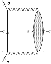
Figure 2: Principal contribution to the dynamical $\Sigma_{\sigma}(\omega)$. Same notation as in figure 1; the transverse spin polarization propagator (see text) is shown as hatched.

$$\Sigma_{\sigma}(\omega)=U^{2}\int_{-\infty}^{\infty}\frac{\mbox{d}\omega_{1}}{2\pi\mbox{i}}\ {\cal G}_{-\sigma}(\omega-\omega_{1})\Pi^{-\sigma\sigma}(\omega_{1}).$$ (4.11)

Here $\Pi^{\sigma-\sigma}(\omega)$ is the transverse spin polarization propagator given by an RPA-like particle-hole ladder sum in the transverse spin channel,

$$\Pi^{\sigma-\sigma}(\omega)=\ ^{0}\Pi^{\sigma-\sigma}(\omega)[1-U^{0}\Pi^{\sigma-\sigma}(\omega)]^{-1}$$ (4.12)

where ${}^{0}\Pi^{\sigma-\sigma}(\omega)$ is the bare particle-hole bubble, itself expressed in terms of the broken symmetry MF propagators $\{{\cal{G}}_{\sigma}\}$ and satisfying the Hilbert transform

$${}^{0}\Pi^{+-}(\omega)=\int_{-\infty}^{\infty}\frac{\mbox{d}\omega_{1}}{\pi}\ \frac{\mbox{Im}^{0}\Pi^{+-}(\omega_{1})\mbox{sgn}(\omega_{1})}{\omega_{1}-\omega^{+}}.$$ (4.13)

We add futher that since [15,27] $\Pi^{+-}(\omega)=\Pi^{-+}(-\omega)$ (and likewise for the ${}^{0}\Pi^{\sigma-\sigma}(\omega)$), only $\Pi^{+-}(\omega)$ need be considered henceforth.

The functional dependence of the $\{\tilde{\Sigma}_{\sigma}(\omega)\}$ on the MF propagators, for both the GFL and LM phases, remains as detailed in [15] for the symmetric model. For the GFL phase in particular, $\Pi^{+-}(\omega)$ obeys the same Hilbert transform equation (4.13) as ${}^{0}\Pi^{+-}$ and equation (4.11) may thus be written as

$$\Sigma_{\sigma}(\omega)=U^{2}\int_{-\infty}^{\infty}\frac{\mbox{d}\omega_{1}}{\pi}\ \mbox{Im}\Pi^{+-}(\sigma\omega_{1})\left[\theta(\omega_{1}){\cal G}_{-\sigma}^{-}(\omega_{1}+\omega)+\theta(-\omega_{1}){\cal G}_{-\sigma}^{+}(\omega_{1}+\omega)\right]$$ (4.14)

where

$${\cal G}_{\sigma}^{\pm}(\omega)=\int_{-\infty}^{\infty}\mbox{d}\omega_{1}\ \frac{D^{0}_{\sigma}(\omega_{1})\theta(\pm\omega_{1})}{\omega-\omega_{1}\pm\mbox{i}0^{+}}$$ (4.15)

denote the one-sided Hilbert transforms such that ${\cal{G}}_{\sigma}(\omega)={\cal{G}}_{\sigma}^{+}(\omega)+{\cal{G}}_{\sigma}^{-}(\omega)$.

Stability

The Hilbert transform equation (4.13) for $\Pi^{+-}(\omega)$ implies the stability condition $\pi$Re$\Pi^{+-}(\omega=0)=\int^{\infty}_{-\infty}\mbox{d}\omega_{1}$Im$\Pi^{+-}(\omega_{1})/|\omega_{1}|>0$. From equation (4.12), together with Im${}^{0}\Pi^{+-}(\omega=0)=0$, it follows that this positivity is guaranteed only if $0<U$Re${}^{0}\Pi^{+-}(\omega=0)\leq 1$. An explicit expression for Re${}^{0}\Pi^{+-}(0)$ is however readily obtained [15,27],

$$U\mbox{Re}^{0}\Pi^{+-}(\omega=0)=\frac{|\bar{\mu}(e_{\mbox{\scriptsize{i}}},x)|}{|\mu|}$$ (4.16)

with $|\bar{\mu}(e_{\mbox{\scriptsize{i}}},x)|$ given by equation (4.10a). The pure MF local moment, denoted by $|\mu_{0}|\equiv|\mu_{0}(e_{\mbox{\scriptsize{i}}})|$, is itself given as the self-consistent solution of $|\mu|=|\bar{\mu}(e_{\mbox{\scriptsize{i}}},x=\frac{1}{2}U|\mu|)|$. Equation (4.16) thus shows that the requisite stability is preserved for $|\mu|\geq|\mu_{0}|$, and that the boundary to stability (when $U$Re$\Pi^{+-}(0;e_{\mbox{\scriptsize{i}}},x)=1)$ is precisely the pure MF local moment $|\mu_{0}|$.

When $|\mu|=|\mu_{0}(e_{\mbox{\scriptsize{i}}})|$ it follows from equation (4.16) that Im$\Pi^{+-}(\omega)$ (equation (4.12)) contains a zero-frequency pole. This is of course the essential signature of the doubly degenerate LM phase, considered explicitly in the following section. In the GFL phase by contrast, $|\mu|=|\mu_{0}|+\delta|\mu|$ is determined by symmetry restoration (step (i) of §4.1.1); with $\delta|\mu|>0$ correctly found in practice, as required for stability. In consequence Im$\Pi^{+-}(\omega)$ contains a sharp resonance occurring at a non-zero frequency $\omega=\omega_{\mbox{\scriptsize{m}}}(\equiv\omega_{*})$, the low-energy Kondo scale for the GFL phase. This is all entirely in keeping with the general picture presented hitherto for the symmetric PAIM, see e.g. figure 4 of [15]. As $U$ is increased for any fixed asymmetry $\eta$ in the GFL phase, $\omega_{\mbox{\scriptsize{m}}}$ progressively diminishes ($\delta|\mu|\rightarrow 0$) and vanishes at a critical $U=U_{\mbox{\scriptsize{c}}}(r,\eta)$, where the resonance becomes an isolated pole at $\omega=0$ ($\delta|\mu|=0$). This signals the transition to the LM phase, to which we now turn.

4.3 LM phase

Throughout the LM phase $|\mu|=|\mu_{0}(e_{\mbox{\scriptsize{i}}})|$ and hence $U$Re$\Pi^{+-}(0)=1$. In consequence $\Pi^{+-}(\omega)$ contains an $\omega=0$ spin-flip pole (of weight $Q$), together with a continuum contribution ${}^{\mbox{\scriptsize{S}}}\Pi^{+-}(\omega)$ [15], specifically

$$\Pi^{+-}(\omega)=-\frac{Q}{\omega+\mbox{i}0^{+}}+\ ^{\mbox{\scriptsize{S}}}\Pi^{+-}(\omega)$$ (4.17)

with $Q=[U^{2}(\partial$Re${}^{0}\Pi^{+-}(\omega)/\partial\omega)_{\omega=0}]^{-1}>0$. Im${}^{\mbox{\scriptsize{S}}}\Pi^{+-}(\omega)$ is given by equation (4.12) with $\Pi^{+-}\rightarrow{}^{\mbox{\scriptsize{S}}}\Pi^{+-}$, and the real/imaginary parts of ${}^{\mbox{\scriptsize{S}}}\Pi^{+-}(\omega)$ are again related by the Hilbert transform equation (4.13). The basic form for $\Sigma_{\sigma}(\omega)$ in the LM phase then follows using equation (4.17) in equation (4.11), namely

$$\Sigma_{\sigma}(\omega)=QU^{2}{\cal G}^{-\sigma}_{-\sigma}(\omega)+^{\mbox{\scriptsize{S}}}\!\Sigma_{\sigma}(\omega).$$ (4.18)

where ${}^{\mbox{\scriptsize{S}}}\Sigma_{\sigma}(\omega)$ is given explicitly by equation (4.14) with $\Pi^{+-}\rightarrow{}^{\mbox{\scriptsize{S}}}\Pi^{+-}$.

For any given $U$ and $\eta$ ($=1+2\epsilon_{\mbox{\scriptsize{i}}}/U$) in the LM phase $U>U_{\mbox{\scriptsize{c}}}(r,\eta)$, $e_{\mbox{\scriptsize{i}}}$ is determined by requiring that the change in number of electrons due to addition of the impurity ($n_{\mbox{\scriptsize{imp}}}$, equation (2.6)) is integral, as for the GFL phase discussed in §2.1. Here however we require that $n_{\mbox{\scriptsize{imp}}}=1$, i.e.

$$n_{\mbox{\scriptsize{imp}}}=\frac{2}{\pi}\mbox{Im}\int^{0}_{-\infty}\mbox{d}\omega\ G(\omega)\left[1-\frac{\partial\Delta(\omega)}{\partial\omega}\right]~{}~{}~{}=1$$ (4.19)

in common with the local moment regime of the atomic limit ($\epsilon_{\mbox{\scriptsize{i}}}<0$ and $\epsilon_{\mbox{\scriptsize{i}}}+U>0$) to which we expect the LM phase generally to be connected perturbatively in $V$. Satisfying equation (4.19) within the approach presented thus determines $e_{\mbox{\scriptsize{i}}}$ in a manner directly analogous to use of the Luttinger theorem to determine $e_{\mbox{\scriptsize{i}}}$ for the GFL phase as described in §4.1.1 (and in fact $n_{\mbox{\scriptsize{imp}}}=1$ is found in practice to be the only possible integer solution for $n_{\mbox{\scriptsize{imp}}}$ in the LM phase).

Symmetry is not of course restored in the doubly degenerate LM phase, i.e. $\tilde{\Sigma}^{\mbox{\scriptsize{R}}}_{\uparrow}(\omega=0)\neq\tilde{\Sigma}^{\mbox{\scriptsize{R}}}_{\downarrow}(\omega=0)$. The difference $\tilde{\Sigma}^{\mbox{\scriptsize{R}}}_{\uparrow}(0)-\tilde{\Sigma}^{\mbox{\scriptsize{R}}}_{\downarrow}(0)$ is however found to be sign definite for all $U>U_{\mbox{\scriptsize{c}}}$; such that as $U$ is decreased towards $U_{\mbox{\scriptsize{c}}}$, $|\tilde{\Sigma}^{\mbox{\scriptsize{R}}}_{\uparrow}(0)-\tilde{\Sigma}^{\mbox{\scriptsize{R}}}_{\downarrow}(0)|$ progressively diminishes and vanishes as the transition is approached, $U\rightarrow U_{\mbox{\scriptsize{c}}}+$. In this way the phase boundary between LM and GFL phases may be established, now coming from the LM side of the transition $U>U_{\mbox{\scriptsize{c}}}$. And the resultant $U_{\mbox{\scriptsize{c}}}\equiv U_{\mbox{\scriptsize{c}}}(r,\eta)$ is correctly found to coincide precisely with that obtained coming from the GFL side, $U<U_{\mbox{\scriptsize{c}}}$, as the limit of solution of the symmetry restoration condition equation (4.5) for the GFL phase (as indeed is to be expected since as $U\rightarrow U_{\mbox{\scriptsize{c}}}+$, the resultant vanishing of $|\tilde{\Sigma}^{\mbox{\scriptsize{R}}}_{\uparrow}(0)-\tilde{\Sigma}^{\mbox{\scriptsize{R}}}_{\downarrow}(0)|$ corresponds to the ‘onset’ of symmetry restoration).

5 Scales, exponents and phase boundaries

We turn now to results arising from the LMA specified above. Single-particle dynamics will be analysed explicitly in §6ff. Here the behaviour of the relevant low-energy scales in the vicinity of the quantum critical point is first considered, followed in §5.2 by resultant phase diagrams in the $(U,\eta)$ (or equivalently $(U,\epsilon_{\mbox{\scriptsize{i}}}))$ plane.

5.1 Scales

Our aim here is simply to establish the critical behaviour of the relevant low-energy scales, specifically $\omega_{*}$ (in terms of which single-particle dynamics exhibit universal scaling (§s 3,6,7)); and, relatedly, the behaviour of the renormalised level $\epsilon_{\mbox{\scriptsize{i}}}^{*}=\epsilon_{\mbox{\scriptsize{i}}}+\Sigma^{\mbox{\scriptsize{R}}}(0)$ (equation (2.14)). Unless stated to the contrary, all results given are representative of the full range $0<r<1$ considered in the paper.

Figure 3: Critical behaviour of the low-energy scale $\omega_{*}$ in the vicinity of the QCP; illustrated for $r=0.3$ and asymmetry $\eta=0.2$ (critical $U_{\mbox{\scriptsize{c}}}\simeq 12.2$, solid square). $\omega_{*}^{r}$ vs $U$ is shown: for $U<U_{\mbox{\scriptsize{c}}}$ (GFL phase, $\omega_{*}\equiv\omega_{\mbox{\scriptsize{m}}}$), $[\omega_{\mbox{\scriptsize{m}}}/U]^{r}$ vs $U$ is plotted (open circles); for $U>U_{\mbox{\scriptsize{c}}}$ (LM phase, $\omega_{*}\equiv\omega_{\mbox{\scriptsize{L}}}$), $|\tilde{\Sigma}^{\mbox{\scriptsize{R}}}_{\uparrow}(0)-\tilde{\Sigma}^{\mbox{\scriptsize{R}}}_{\downarrow}(0)|\propto\omega_{*}^{r}$ is plotted (open squares). In either case, $\omega_{*}\sim|U-U_{\mbox{\scriptsize{c}}}|^{\frac{1}{r}}$ as the transition is approached. See text for further details.

We begin by considering the GFL phase, $U<U_{\mbox{\scriptsize{c}}}$. The critical behaviour of the low-energy Kondo scale $\omega_{\mbox{\scriptsize{m}}}\equiv\omega_{*}$ is illustrated in figure 3 for $r=0.3$ and an asymmetry $\eta=1-2|\epsilon_{\mbox{\scriptsize{i}}}|/U=0.2$; the critical $U_{\mbox{\scriptsize{c}}}(r,\eta)\simeq 12.2$ being marked as a solid square. Specifically, $(\omega_{\mbox{\scriptsize{m}}}/U)^{r}$ vs $U$ (open circles) is shown, and seen to vanish linearly as $U\rightarrow U_{\mbox{\scriptsize{c}}}-$. The critical exponent $a$ of §3 ($\omega_{*}\sim u^{a}$ with $u=|1-U/U_{\mbox{\scriptsize{c}}}|)$ is thus $a=1/r$, which agrees with the NRG calculations of [18] (the result is also derivable analytically for $r\ll 1$, see §7.1). We find also that $\omega_{*}\equiv\omega_{\mbox{\scriptsize{m}}}$ and the quasiparticle weight $Z$ are indeed related by equation (3.8), namely that $Z\sim\omega_{*}^{1-r}\sim u^{(1-r)/r}$ as $u\rightarrow 0$.

As argued in §3, the renormalised level $\epsilon_{\mbox{\scriptsize{i}}}^{*}$ should likewise vanish as the transition is approached, from either phase. When considering the LM phase in particular it will in general prove helpful to define spin-dependent renormalised levels via

$$\epsilon_{\mbox{\scriptsize{i}}\sigma}^{*}=\epsilon_{\mbox{\scriptsize{i}}}+\tilde{\Sigma}^{\mbox{\scriptsize{R}}}_{\sigma}(\omega=0).$$ (5.20)

The two-self-energies $\{\tilde{\Sigma}_{\sigma}^{\mbox{\scriptsize{R}}}(\omega)\}$ are related to the conventional single self-energy $\Sigma(\omega)$ by equation (2.11), from which the $\{\epsilon_{\mbox{\scriptsize{i}}\sigma}^{*}\}$ and the renormalised level $\epsilon_{\mbox{\scriptsize{i}}}^{*}=\epsilon_{\mbox{\scriptsize{i}}}+\Sigma^{\mbox{\scriptsize{R}}}(0)$ are related by

$$\epsilon_{\mbox{\scriptsize{i}}}^{*}=\frac{\epsilon_{\mbox{\scriptsize{i}}\uparrow}^{*}\epsilon_{\mbox{\scriptsize{i}}\downarrow}^{*}}{\frac{1}{2}[\epsilon_{\mbox{\scriptsize{i}}\uparrow}^{*}+\epsilon_{\mbox{\scriptsize{i}}\downarrow}^{*}]}.$$ (5.21)

In the GFL phase (where symmetry is restored, $\tilde{\Sigma}^{\mbox{\scriptsize{R}}}_{\uparrow}(0)=\tilde{\Sigma}^{\mbox{\scriptsize{R}}}_{\downarrow}(0)$) the renormalised levels all coincide, $\epsilon_{\mbox{\scriptsize{i}}}^{*}=\epsilon_{\mbox{\scriptsize{i}}\sigma}^{*}$. For the LM phase by contrast, $\epsilon_{\mbox{\scriptsize{i}}}^{*},\epsilon_{\mbox{\scriptsize{i}}\uparrow}^{*}$ and $\epsilon_{\mbox{\scriptsize{i}}\downarrow}^{*}$ are in general distinct.

Figure 4: Renormalised level $\epsilon_{\mbox{\scriptsize{i}}}^{*}=\epsilon_{\mbox{\scriptsize{i}}}+\Sigma^{\mbox{\scriptsize{R}}}(0)$ vs $U$ in the vicinity of the QCP for $r=0.3$ and $\eta=0.2$. GFL phase points ($U<U_{\mbox{\scriptsize{c}}}$) are shown as circles, LM phase as squares. In the LM phase the $\uparrow/\downarrow$-spin renormalised levels $\epsilon_{\mbox{\scriptsize{i}}\sigma}^{*}=\epsilon_{\mbox{\scriptsize{i}}}+\tilde{\Sigma}^{\mbox{\scriptsize{R}}}_{\sigma}(0)$ are also shown, as up/down triangles. All vanish linearly as the transition is approached.

Figure 4, again for $r=0.3$ and $\eta=0.2$, shows the resultant $U$-dependence of $\epsilon_{\mbox{\scriptsize{i}}}^{*}$ (open circles for $U<U_{\mbox{\scriptsize{c}}}$ in the GFL phase, squares for $U>U_{\mbox{\scriptsize{c}}}$). The renormalised level is indeed seen to vanish as the transition is approached from either phase, with an exponent $a_{1}=1$ ($|\epsilon_{\mbox{\scriptsize{i}}}^{*}|\sim u^{a_{1}}$), in agreement with the inferences drawn in §3. For the GFL phase in particular, $\omega_{*}\equiv\omega_{\mbox{\scriptsize{m}}}$ and $|\epsilon_{\mbox{\scriptsize{i}}}^{*}|$ are thus related by equation (3.11), $|\epsilon_{\mbox{\scriptsize{i}}}^{*}|=k\omega_{*}^{r}$ (and where the constant $k\equiv k(\eta)$ is an odd function of the asymmetry $\eta$, such that $\epsilon_{\mbox{\scriptsize{i}}}^{*}=0$ by symmetry (§3) for the GFL phase of the particle-hole symmetric PAIM, $\eta=0$). For the LM phase $U>U_{\mbox{\scriptsize{c}}}$, figure 4 also shows the spin-dependent renormalised levels $\epsilon_{\mbox{\scriptsize{i}}\sigma}^{*}$ (triangles); each being seen to be sign definite and to vanish linearly as $U\rightarrow U_{\mbox{\scriptsize{c}}}+$.

For the GFL phase, the low-energy (Kondo) scale $\omega_{*}\equiv\omega_{\mbox{\scriptsize{m}}}$ arises as a direct consequence of symmetry restoration. The reader will however notice that the corresponding scale $\omega_{*}$ for the LM phase, in terms of which single-particle dynamics exhibit scaling and denoted by $\omega_{*}\equiv\omega_{\mbox{\scriptsize{L}}}$, has not yet been specified. Here we simply assert, and consider further in §s 6ff, that $\omega_{\mbox{\scriptsize{L}}}$ is related to the spin-dependent renormalised levels by

$$\omega_{*}\equiv\omega_{\mbox{\scriptsize{L}}}\propto|\epsilon_{\mbox{\scriptsize{i}}\uparrow}^{*}-\epsilon_{\mbox{\scriptsize{i}}\downarrow}^{*}|^{\frac{1}{r}}=|\tilde{\Sigma}^{\mbox{\scriptsize{R}}}_{\uparrow}(0)-\tilde{\Sigma}^{\mbox{\scriptsize{R}}}_{\downarrow}(0)|^{\frac{1}{r}}$$ (5.22)

(or equivalently by $\omega_{\mbox{\scriptsize{L}}}\propto|\epsilon_{\mbox{\scriptsize{i}}\sigma}^{*}|^{\frac{1}{r}}$; which equivalence follows since each $\epsilon_{\mbox{\scriptsize{i}}\sigma}^{*}$ vanishes linearly as $U\rightarrow U_{\mbox{\scriptsize{c}}}+$, figure 4, and low-energy scales are equivalent up to an arbitrary constant. The specific proportionality employed in practice will also be specified in §6.2). Figure 3 also shows $|\tilde{\Sigma}_{\uparrow}^{\mbox{\scriptsize{R}}}(0)-\tilde{\Sigma}_{\downarrow}^{\mbox{\scriptsize{R}}}(0)|\propto\omega_{\mbox{\scriptsize{L}}}^{r}$ for $U>U_{\mbox{\scriptsize{c}}}$ (open squares); the overall figure thus showing the $U$-dependence of $\omega_{*}^{r}$ in both phases.

5.2 Phase diagrams

We now consider representative phase diagrams arising from the LMA, obtained as described in §4. As usual the range $0<r<1$ is considered; and we show in particular that the essential characteristics of the phase diagrams divide into two classes, namely $r<\frac{1}{2}$ and $r>\frac{1}{2}$.

Figure 5: LMA phase boundary in the $(U,\epsilon_{\mbox{\scriptsize{i}}})$-plane for a fixed $r=0.2$ (solid line), representative of the general behaviour for $r<\frac{1}{2}$. The dashed line marks the particle-hole symmetric case: $U=-2\epsilon_{\mbox{\scriptsize{i}}}$. The corresponding MF phase boundary is shown as a dotted line.

Figure 5 shows behaviour typical of $r<\frac{1}{2}$, the phase boundary in the $(U,\epsilon_{\mbox{\scriptsize{i}}})$-plane for a fixed $r=0.2$. As $\epsilon_{\mbox{\scriptsize{i}}}$ is progressively increased, the critical $U_{\mbox{\scriptsize{c}}}\equiv U_{\mbox{\scriptsize{c}}}(r,\epsilon_{\mbox{\scriptsize{i}}})$ (solid line) first decreases, reaches a minimum at the particle-hole symmetric line $\epsilon_{\mbox{\scriptsize{i}}}=-\frac{1}{2}U$ (shown as a dashed line), before rising sharply at $\epsilon_{\mbox{\scriptsize{i}}}\simeq-5$ and eventually turning back on itself. This has two interesting consequences. First that the LM phase is inaccessible by increasing $U$ for any fixed $\epsilon_{\mbox{\scriptsize{i}}}\gtrsim-5$ in the present example. Second, for fixed $\epsilon_{\mbox{\scriptsize{i}}}$ and due to the above ‘turnback’, there is at large $U$ a re-entrant transition back to the GFL phase (itself seen most clearly in figure 18 below, where a low-$r$ phase boundary determined analytically in §7.1 is shown). Both observations are in general accord with results of recent NRG calculations [36]; and indeed are seen even at the pure MF level of unrestricted Hartree-Fock, shown in figure 5 as a dotted line (although the LM phase is strongly exaggerated by pure MF, the many qualitative deficiencies of which are discussed e.g. in [15,25,27]).

Figure 6: Phase diagram in the $(U,\eta)$-plane for $r=0.2$: $\eta$ vs $(8/\pi r)U^{r-1}$ is shown (solid line). The corresponding $r\rightarrow 0$ result, obtained analytically in §7.1, is also shown (dashed line); see §7.1 for full discussion.

A rather more revealing portrayal of the phase boundary for fixed $r$ is shown in figure 6 where, for $r=0.2$, $U_{\mbox{\scriptsize{c}}}\equiv U_{\mbox{\scriptsize{c}}}(r,\eta)$ is displayed as a function of the asymmetry $\eta$. Specifically, $\eta$ vs $(8/\pi r)U_{\mbox{\scriptsize{c}}}^{r-1}(r,\eta)$ is shown; the constant $8/\pi r$ simply serving as a convenient ‘normalisation’, it being known from previous LMA work [15] that as $r\rightarrow 0$, $U_{\mbox{\scriptsize{c}}}^{r-1}(r,0)\sim\pi r/8$ for the symmetric PAIM $\eta=0$ (which result is exact [15,16]). In contrast to $U_{\mbox{\scriptsize{c}}}(r,\epsilon_{\mbox{\scriptsize{i}}})$ shown in figure 5, which is not single-valued in $\epsilon_{\mbox{\scriptsize{i}}}$ (leading to re-entrance as above), figure 6 shows $U_{\mbox{\scriptsize{c}}}(r,\eta)$ to be a single-valued function of the asymmetry (which is found for all $r$); and that LM states are always accessible upon increasing $U$ for any fixed asymmetry $|\eta|<1$. In §7.1 the $\eta$-dependence of $U_{\mbox{\scriptsize{c}}}(r,\eta)$ arising within the LMA will be discussed further and obtained analytically in the small-$r$ limit (which result is also shown in figure 6).

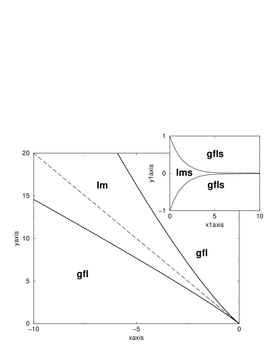
Figure 7: Main figure: LMA phase boundary in the $(U,\epsilon_{\mbox{\scriptsize{i}}})$-plane for $r=0.7$, respresentative of the general behaviour for $r>\frac{1}{2}$. The dashed line marks the symmetric limit, $U=-2\epsilon_{\mbox{\scriptsize{i}}}$; in this case $(\eta=0)$ only LM states are accessible. Inset: phase boundary in the $(U,\eta)$-plane, $\eta$ vs ($8/\pi r)U^{r-1}$ being shown.

Figure 6 also shows clearly that particle-hole symmetry is optimal for LM formation — $\eta=0$ corresponding to the lowest critical $U_{\mbox{\scriptsize{c}}}(r,\eta)$. For the symmetric model it is however well known [10-20] that for $r>1/2$ the GFL phase does not survive for any non-zero $U$. It is for this reason that phase diagrams for $r\lessgtr 1/2$ are distinct, and figure 7 illustrates the point. For $r=0.7$ the main figure (cf figure 5) shows the critical $U_{\mbox{\scriptsize{c}}}(r,\epsilon_{\mbox{\scriptsize{i}}})$ vs $\epsilon_{\mbox{\scriptsize{i}}}$; from which in particular the re-entrant behaviour upon increasing $U$ for fixed $\epsilon_{\mbox{\scriptsize{i}}}$ is again apparent. And the inset to figure 7 shows the $\eta$-dependence of the phase boundary (in direct parallel to figure 6). The qualitative differences between the $r<1/2$ and $r>1/2$ phase boundaries are self-evident.

Figure 8: $r$-dependence of the phase boundaries for fixed asymmetry $\eta$: $U^{-1}$ vs $r$ for (from top to bottom) $\eta=0.1,0.2,0.3,0.4$ and $0.5$. See text for details. Since the wide-band limit ($D=\infty$) is employed here, the largest $r$ considered in practice is $r=0.95$.

The $r$-dependence of the phase boundaries is illustrated in figure 8, which shows $U_{\mbox{\scriptsize{c}}}^{-1}(r,\eta)$ vs $r$ for a range of asymmetries $\eta$. For $\eta>0$ the resultant phase boundaries have a maximum — in qualitative accord with the NRG results of [13] for $U=\infty$ — which moves to lower $r$ with increasing $\eta$. For the symmetric case $\eta=0$ the present approach is known [15] to be deficient as $r\rightarrow 1/2$, in not capturing the slow (logarithmic) divergence of $U_{\mbox{\scriptsize{c}}}^{-1}(r\rightarrow\frac{1}{2},0)$ seen in NRG calculations [12,13,16]; in turn reflecting the neglect of charge fluctuations in the present LMA (which are necessarily important in this limit, since $U_{\mbox{\scriptsize{c}}}(r\rightarrow\frac{1}{2},0)\rightarrow 0$). We do not however doubt at least the qualitative validity of the results shown for $\eta>0$ where $U_{\mbox{\scriptsize{c}}}(r,\eta)$ remains finite for all $r$ considered.

Finally, note from figure 8 that for small $r$ the critical $U_{\mbox{\scriptsize{c}}}^{-1}(r,\eta)\propto r$ for fixed asymmetry, with a coefficient that is largest in the particle-hole symmetric case $\eta=0$. We will revisit the matter analytically in §7.1, and show that this behaviour is intimately related to the exponential asymptotics of the ubiquitously non-vanishing Kondo scale characteristic of the $r=0$ metallic impurity model.

6 Single-particle dynamics

We turn now to LMA results arising for single-particle dynamics, on all relevant energy scales and including in particular the many different facets of their scaling behaviour as the underlying quantum phase transition is approached. The GFL and LM phases are considered separately in §s 6.1 and 6.2 respectively, and dynamics precisely at the QCP in §6.3.

6.1 GFL phase

A typical GFL phase spectrum is given in figure 9: $\pi D(\omega)$ vs $\omega$, shown for $r=0.3$, an asymmetry $\eta=1+2\epsilon_{\mbox{\scriptsize{i}}}/U=0.2$ and an interaction strength $U=11$ close to the critical $U_{\mbox{\scriptsize{c}}}(r,\eta)\simeq 12.2$. Note first that the change in number of electrons due to addition of the impurity is correctly $n_{\mbox{\scriptsize{imp}}}=0$, as required by the Freidel sum rule equation (4.8) (where $\epsilon_{\mbox{\scriptsize{i}}}^{*}=\epsilon_{\mbox{\scriptsize{i}}}+\tilde{\Sigma}^{\mbox{\scriptsize{R}}}_{\sigma}(0)>0$ for $\eta>0$). By contrast, the local impurity charge $n=2\int^{0}_{-\infty}\mbox{d}\omega D(\omega)$ is $n\simeq 0.96$, close to the Kondo limit where $n\rightarrow 1$; showing in turn (since $n_{\mbox{\scriptsize{imp}}}=0$) that essentially one electron is transferred from the conduction band to the impurity upon its addition to the host.

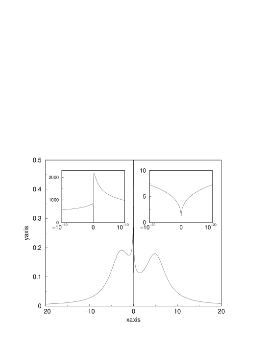
Figure 9: GFL phase spectrum for $r=0.3$, asymmetry $\eta=0.2$ and interaction $U=11$ (the critical $U_{\mbox{\scriptsize{c}}}(r,\eta)\simeq 12.2$): $\pi D(\omega)$ vs $\omega$. Insets: spectral behaviour on the lowest energy scales. See text for discussion.

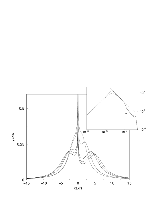
Figure 10: GFL phase spectral evolution with $U$, for $r=0.3$ and $\eta=0.2$ (the critical $U_{\mbox{\scriptsize{c}}}\simeq 12.2$): $\pi D(\omega)$ vs $\omega$ for $U=11,10,9,6$ and $5$ in obvious sequence. Inset: $\pi D(\omega)$ vs $|\omega|$ on a logarithmic scale, for both $\omega>0$ (solid line) and $\omega<0$ (dashed). $\omega=\omega_{*}$ ($\equiv\omega_{\mbox{\scriptsize{m}}}$) is indicated by a vertical arrow. The function cos${}^{2}(\frac{\pi}{2}r)|\omega|^{-r}$ is also shown (dotted line); see text for full discussion.

On high energy scales the expected Hubbard satellites are seen in the spectrum, centred on $\omega\simeq\epsilon_{\mbox{\scriptsize{i}}}$ and $\epsilon_{\mbox{\scriptsize{i}}}+U$; and correctly broadened two-fold over their counterparts at pure MF level for the physical reasons discussed in [15,25]. Spectral evolution with $U$ is illustrated in figure 10 where, for the same $r$ and $\eta$, the spectra are shown upon decreasing $U$ further from the phase boundary into the GFL phase. With diminishing interaction the Hubbard satellites become progressively less pronounced as expected, and ultimately absorbed into the central resonance structure. It is the latter that we now begin to consider in more detail, focusing first on the lowest energy behaviour.

The left-hand inset of figure 9 shows the low-energy behaviour of the spectrum on a greatly expanded scale. It consists of two pronounced peaks of unequal intensity, one either side of the Fermi level $\omega=0$, with the more intense peak arising for $\omega>0$. This is quite general, applying for all $\eta>0$ (where $n_{\mbox{\scriptsize{imp}}}=0$) and $r$, for $U$ close to $U_{\mbox{\scriptsize{c}}}(r,\eta)$. For $\eta<0$ this situation is reversed: under $\eta\rightarrow-\eta$ as discussed in §2, the spectrum is simply reflected, $D(\omega,\eta)=D(-\omega,-\eta)$ (and $n_{\mbox{\scriptsize{imp}}}=0\rightarrow 2-n_{\mbox{\scriptsize{imp}}}=2$). The greater peak then lies below, and the lesser above, the Fermi level. For any asymmetry $\eta\neq 0$, where $\epsilon_{\mbox{\scriptsize{i}}}^{*}\neq 0$ in the GFL phase, $D(\omega)$ has the ultimate low-$\omega$ behaviour $D(\omega)\propto|\omega|^{r}$; given trivially (e.g. from equation (3.9)) by

$$\pi D(\omega)\stackrel{{\scriptstyle\omega\rightarrow 0}}{{\sim}}\frac{|\omega|^{r}}{{}\epsilon_{\mbox{\scriptsize{i}}}^{*}{}^{2}}$$ (6.1)

and symmetric in $\omega$. This is illustrated in the right inset to figure 9 (and is of course in contrast to the symmetric PAIM [12,14-16,18,20] $\eta=0$ (and $\epsilon_{\mbox{\scriptsize{i}}}^{*}=0$), for which $D(\omega)\propto|\omega|^{-r}$ as $|\omega|\rightarrow 0$, equation (3.5)).

The qualitative features of the preceding paragraph are in agreement with results of recent NRG calculations [18]. We now show that they may be understood using the simple low-$\omega$ quasiparticle form for the impurity spectrum, discussed in §3, that is characteristic of the GFL phase. Following that however, we point out the severe inadequacies of the quasiparticle form in understanding the GFL phase scaling spectrum on all relevant frequency scales, and in particular its essential irrelevance in understanding the behaviour of the spectrum at the quantum critical point (which itself is considered in §’s 6.3,7.2).

The quasiparticle spectrum is given in scaling form by equation (3.9), as a function of $\tilde{\omega}=\omega/\omega_{*}$ with $\omega_{*}=\omega_{\mbox{\scriptsize{m}}}$ the low-energy Kondo spin-flip scale characteristic of the GFL phase (determined via symmetry restoration as described in §4); and with $k_{1}=\omega_{*}^{1-r}/Z$ (equation (3.8)) a constant of order unity as the transition is approached, where $\omega_{*}$ and $Z$ separately vanish (§5). The quasiparticle form is of course restricted by construction to $|\tilde{\omega}|\ll 1$ (which regime is now considered); and for present purposes equation (3.9) may be replaced with negligible error (as shown below) by

$$\pi\omega_{*}^{r}D(\omega)\simeq\frac{|\tilde{\omega}|^{r}}{[\frac{\epsilon_{\mbox{\scriptsize{i}}}^{*}}{\omega_{*}^{r}}-\mbox{sgn}(\omega)\beta(r)|\tilde{\omega}|^{r}]^{2}+|\tilde{\omega}|^{2r}}$$ (6.2)

where $\beta(r)=$ tan$(\frac{\pi}{2}r)$ as usual (and with $k=|\epsilon_{\mbox{\scriptsize{i}}}^{*}|/\omega_{*}^{r}$ likewise finite as $U\rightarrow U_{\mbox{\scriptsize{c}}}(r,\eta)-$, as shown explicitly in §5). Equivalently and conveniently, equation (6.2) may be recast as

$$\pi|\epsilon_{i}^{*}|D(\omega)\simeq\frac{|\omega^{\prime}|^{r}}{[1-\mbox{sgn}(\omega)\beta(r)|\omega^{\prime}|^{r}]^{2}+|\omega^{\prime}|^{2r}}$$ (6.3)

with $\omega^{\prime}=\omega/{}|\epsilon_{\mbox{\scriptsize{i}}}^{*}|{}^{\frac{1}{r}}$ (and where $\epsilon_{\mbox{\scriptsize{i}}}^{*}>0$ has been taken, as appropriate to $\eta>0$). Equations (6.2) or (6.3) capture the low-energy ‘two-peak’ spectral structure illustrated in the insets to figure 9. Equation (6.1) is of course trivially recovered as $|\omega|\rightarrow 0$; and from equation (6.3) the resultant spectrum has maxima at $\omega=\pm T^{*}$, where

$$T^{*}=[|\epsilon_{\mbox{\scriptsize{i}}}^{*}|cos(\mbox{$\frac{\pi}{2}$}r)]^{\frac{1}{r}}.$$ (6.4)

For any non-zero asymmetry $\eta$, the low-energy scale $T^{*}$ is proportional to $\omega_{*}$ and is thus equivalent to it (as follows from equation (3.11), noting that $k$ $(\equiv k(r,\eta))$ is odd in $\eta$ such that for the particle-hole symmetric model $\eta=0$, $\epsilon_{\mbox{\scriptsize{i}}}^{*}=0$ as in §3). We have here introduced $T^{*}$ simply to make connection to the NRG calculations of [18] for the asymmetric PAIM, where the low-energy scale was defined as the location of the spectral maxima.

Figure 11: Low-frequency GFL scaling spectra: $\pi|\epsilon_{\mbox{\scriptsize{i}}}^{*}|D(\omega)$ vs $\omega/T^{*}$ (with the low-energy scale $T^{*}$ defined in equation (6.4)), shown for $r=0.1$ (dotted line), $0.2$ (short dash), $0.3$ (solid), $0.4$ (long dash) and $0.5$ (point dash). For the case of $r=0.3$, explicit comparison is also made to the approximate quasiparticle form equation (6.3); it is however indistinguishable from the full LMA results (which were obtained explicitly for $\eta=0.2$ but for $\eta\neq 0$ are in fact $\eta$-independent over the $\omega/T^{*}$-range shown, see equation (6.3)).

In figure 11, LMA results for $\pi|\epsilon_{\mbox{\scriptsize{i}}}^{*}|D(\omega)$ as the transition is approached are given, plotted vs $\omega/T^{*}$ for a range of different $r$’s (and noting that in all cases the range $|\omega|/T^{*}<10$ shown corresponds to $|\omega|/\omega_{*}\ll 1$, since the constant $k=|\epsilon_{\mbox{\scriptsize{i}}}^{*}|/\omega_{*}^{r}\sim(T^{*}/\omega_{*})^{r}$ is found in practice to be small compared to unity). We emphasise that the figure shows ‘full’ LMA results; that the spectra are of course scaling spectra, obtained as $U\rightarrow U_{\mbox{\scriptsize{c}}}(r,\eta)-$ and as such universally dependent on $\omega/T^{*}$ (or equivalently $\tilde{\omega}$) alone; and that the exponent $b$ of §3 (equation (3.2)) is indeed $b=r$. As seen from figure 11 the asymmetrically disposed spectral maxima are indeed peaked at $\omega/T^{*}=\pm 1$, and for the particular case of $r=0.3$ the figure compares explicitly the LMA results to the approximate quasiparticle form equation (6.3). This is not perceptibly distinguishable from the full LMA results, showing that equation (6.3) is indeed accurate (the same being true for the other $r$’s shown).

For sufficiently low $\omega/T^{*}$ or $\tilde{\omega}$, the GFL phase scaling spectrum is thus explicable in terms of the simple approximate quasiparticle form equations (6.2) or (6.3). An obvious question then arises: can this form be extrapolated beyond its strict confines, to infer the leading large $\omega/T^{*}$ (or $\tilde{\omega}$) form of the scaling spectrum which — as shown on general grounds in §3 (equations (3.2-4)) — determines the behaviour of the spectrum precisely at the quantum critical point where the low-energy scale $\omega_{*}\propto T^{*}=0$, and the generic form of which is given by equation (3.4)($\pi D(U_{\mbox{\scriptsize{c}}};\omega)=C(r;\eta)|\omega|^{-r})$? The reader will notice for example that the leading high frequency behaviour predicted from equations (6.2,3) is $\pi\omega_{*}^{r}D(\omega)\sim$ cos${}^{2}(\frac{\pi}{2}r)|\tilde{\omega}|^{-r}$; from which the $\omega_{*}$ scale drops out of either side, resulting in an apparent QCP spectrum that is indeed of the required general form equation (3.4), but with a coefficient $C(r,\eta)=$cos${}^{2}(\frac{\pi}{2}r)$. As seen from equation (3.5) the resultant QCP spectrum, if correct, would in fact coincide precisely with the non-interacting limit of the particle-hole symmetric ($\eta=0$) PAIM.

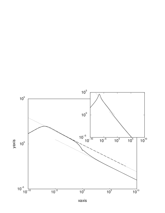
Figure 12: Full GFL phase scaling spectrum for $r=0.3$ and $\eta=0.2$: $\pi\omega_{*}^{r}D(\omega)$ vs $\tilde{\omega}=\omega/\omega_{*}$ ($\omega_{*}\equiv\omega_{\mbox{\scriptsize{m}}}$) plotted for $\tilde{\omega}>0$ on a logarithmic scale (solid line) and encompassing all relevant $\tilde{\omega}$ regimes. The approximate quasiparticle form equation (6.2) is shown as a dashed line; the upper dotted line shows the $\eta=0$ non-interacting behaviour cos${}^{2}(\frac{\pi}{2}r)|\tilde{\omega}|^{-r}$. For $|\tilde{\omega}|\gg 1$ the ultimate high-frequency behaviour of the scaling spectrum is also $\propto|\tilde{\omega}|^{-r}$ but with a different coefficient $C(r,\eta)$ that is $r$- and $\eta$-dependent; the lower dotted line shows the latter behaviour extrapolated back to lower $\tilde{\omega}$. Full discussion in text. Inset: corresponding results for $r=0.7$ and $\eta=0.4$, same notation as main figure.

The latter conclusions are not in fact correct, but the above discussion is nonetheless informative as now shown. Figure 12 gives the full LMA scaling spectrum for $r=0.3$ and $\eta=0.2$: $\pi\omega_{*}^{r}D(\omega)$ for $\omega>0$ (solid line) as a function of $\tilde{\omega}=\omega/\omega_{*}$, on a logarithmic scale encompassing the entire relevant $\tilde{\omega}$ range (and with $\tilde{\omega}=1$ seen as a small ‘dip’ in the spectrum, a well known and harmless artefact of the RPA-like form for $\Pi^{+-}$ employed here [15,25-27]). The figure also shows the approximate quasiparticle form equation (6.2) (dashed line), together with its asymptotic behaviour $\pi\omega_{*}^{r}D(\omega)\sim$cos${}^{2}(\frac{\pi}{2}r)|\tilde{\omega}|^{-r}$ mentioned above (upper dotted line). The full LMA scaling spectrum is well captured by the quasiparticle form up to $\tilde{\omega}\simeq 10^{-1}$, below which is indeed seen to exist an appreciable ‘intermediate’ $\tilde{\omega}$-range over which the behaviour $\pi\omega_{*}^{r}D(\omega)\sim$cos${}^{2}(\frac{\pi}{2}r)|\tilde{\omega}|^{-r}$ clearly arises. For larger frequencies however, the scaling spectrum clearly departs from $\sim$cos${}^{2}(\frac{\pi}{2}r)|\tilde{\omega}|^{-r}$ behaviour; and for $\tilde{\omega}\gg 1$ is seen to cross over into ultimate large-$\tilde{\omega}$ behaviour that is again $\propto|\tilde{\omega}|^{-r}$ — following generally from the fact that the exponent $b=r$ as explained in §3 — but with a prefactor $C(r,\eta)$ that differs from cos${}^{2}(\frac{\pi}{2}r)$ and is found in practice to be $\eta$-dependent.

The above behaviour is not particular to the case $r=0.3$ illustrated, being found to arise throughout the range $0<r<1$ considered (the inset to figure 12 shows corresponding results for $r=0.7$ and $\eta=0.4$). The asymmetric GFL phase scaling spectrum thus contains two regimes of $\sim|\tilde{\omega}|^{-r}$ behaviour: that at lower $\tilde{\omega}$ ($\ll 1$) corresponds to symmetric ($\eta=0$) non-interacting limit behaviour, while that arising for $\tilde{\omega}\gg 1$ determines the QCP spectrum. This ‘two $|\tilde{\omega}|^{-r}$ regime’ behaviour is in fact known [20] to arise also in the pure symmetric PAIM, $\eta=0$ (where the cos${}^{2}(\frac{\pi}{2}r)|\tilde{\omega}|^{-r}$ regime persists all the way down to $\omega=0$, reflecting the exact low-$\omega$ behaviour equation (3.5) arising in that case). Further consideration of the matter will be given in §6.3, and the $(r,\eta)$-dependence of the QCP spectrum arising within the LMA will be determined analytically for small $r$ in §7.2.

Finally, we point out that figure 12 shows the scaling spectrum for $\omega>0$, but that it is not of course symmetric in $\tilde{\omega}$ (or $\omega/T^{*}$) as is obvious e.g. from figure 11. The sgn($\omega$)-dependence of the GFL phase spectrum is illustrated further in the inset to figure 10 above (for $[r,\eta]=[0.3,0.2]$ and $U=11$, quite close to $U_{\mbox{\scriptsize{c}}}\simeq 12.2$). Here the spectrum $\pi D(\omega)$ vs $|\omega|$ (i.e. unscaled) is again shown on a log-scale, for both $\omega>0$ (solid line) and $\omega<0$ (dashed). For each sgn($\omega$) the above ‘intermediate’ behaviour $\sim$cos${}^{2}(\frac{\pi}{2}r)|\omega|^{-r}$ arises (shown as a dotted line). Beyond that however, a crossover to $\sim C(r,\eta)|\omega|^{-r}$ behaviour occurs; with the $C(r,\eta)$ dependent not only on $r$ and $\eta$ but also for $\eta\neq 0$ on sgn($\omega$) (which behaviour we add is not precluded by the general considerations of §3, and which is likewise considered further in the following sections). Since the spectrum here is shown in unscaled form the non-universal Hubbard satellites are also ultimately visible on the figure, likewise asymmetrically disposed about $\omega=0$ because $\eta\neq 0$. We also add here that while results from the present LMA are in general agreement with the NRG calculations of [18], there is one point on which we differ. That we find the coefficient $C(r,\eta)$ to depend on $\eta$ (albeit fairly weakly), is consistent with a line of ($\eta$-dependent) critical fixed points. Numerical RG calculations for the pseudogap Kondo model [13] appear by contrast to be consistent for any $\eta>0$ with a single critical fixed point, and hence in effect no $\eta$-dependence in $C(r,\eta)$.

6.2 LM phase

We turn now to the LM phase, considering first spectral evolution on ‘all scales’ as $U$ is progressively decreased for fixed asymmetry $\eta$, towards the LM/GFL transition at $U_{\mbox{\scriptsize{c}}}(r,\eta)$. This is illustrated in figure 13, again for $r=0.3$ and $\eta=0.2$ ($U_{\mbox{\scriptsize{c}}}\simeq 12.2$), although the behaviour shown is representative of the full $r$-range considered. $\pi D(\omega)$ vs $\omega$ is shown, for $U=50,20,17$ and $14$.

Figure 13: LM phase spectral evolution with $U$, for $r=0.3$ and $\eta=0.2$ ($U_{\mbox{\scriptsize{c}}}\simeq 12.2$): $\pi D(\omega)$ vs $\omega$ for $U=50,20,17,14$ (clockwise from top left).

For the highest $U$ shown, deep in the LM phase, the well developed Hubbard satellites dominate the spectrum entirely, although the ultimate low-$\omega$ spectral behaviour vanishes as $\propto|\omega|^{r}$ throughout the LM phase as noted in §3. With decreasing $U$ however, a low-energy spectral structure is seen to develop in the vicinity of the Fermi level. It becomes increasingly pronounced as $U\rightarrow U_{\mbox{\scriptsize{c}}}+$ and as shown below is the precursor, in the LM phase, of the $|\omega|^{-r}$ divergent behaviour characteristic of the QCP itself.

For $U=12.3$, close to $U_{\mbox{\scriptsize{c}}}$, $\pi D(\omega)$ vs $\omega$ is shown in figure 14; the left inset showing the low-energy part of the spectrum. The latter is clearly redolent of its counterpart for the GFL phase (figure 9), the

Figure 14: LM phase spectrum $\pi D(\omega)$ vs $\omega$ for $r=0.3$, $\eta=0.2$ and interaction $U=12.3$ close to the critical $U_{\mbox{\scriptsize{c}}}\simeq 12.2$. Left inset: low-energy behaviour on an expanded scale. Right inset: $\pi D(\omega)$ vs $|\omega|$ on a logarithmic scale, for both $\omega>0$ (solid line) and $\omega<0$ (dashed). Full discussion in text.

low-energy behaviour again consisting of two peaks of unequal intensity, the more intense peak arising for $\omega>0$ (and vice versa for $\eta<0$). In contrast to the GFL phase however, the positions of the peak maxima are not symmetrically disposed about the Fermi level; reflecting the fact that in the LM phase, where symmetry is not restored, the spin-dependent renormalised levels $\epsilon_{\mbox{\scriptsize{i}}\sigma}^{*}=\epsilon_{\mbox{\scriptsize{i}}}+\tilde{\Sigma}^{\mbox{\scriptsize{R}}}_{\sigma}(\omega=0)$ do not coincide (as shown e.g. in figure 4). In addition, and again in contrast to the GFL phase, we find within the LMA that while the lowest-$\omega$ spectral behaviour is $\propto|\omega|^{r}$ as noted above, the coefficient thereof depends on sgn($\omega$). The origins of this are readily seen using equations (2.9,10), which give the leading low-$\omega$ behaviour

$${\pi D(\omega)\stackrel{{\scriptstyle\omega\rightarrow 0}}{{\sim}}\mbox{$\frac{1}{2}$}}\sum_{\sigma}\frac{[\Delta_{\mbox{\scriptsize{I}}}(\omega)+\Sigma^{\mbox{\scriptsize{I}}}_{\sigma}(\omega)]}{[\epsilon_{\mbox{\scriptsize{i}}\sigma}^{*}]^{2}}$$ (6.5)

with the LM phase $\Sigma_{\sigma}(\omega)$ given explicitly within the LMA considered here by equation (4.18). It is the first term of the latter that controls the low-$\omega$ behaviour of $\Sigma^{\mbox{\scriptsize{I}}}_{\sigma}(\omega)$ which, using equations (4.6,15), is found to be of form $\Sigma^{\mbox{\scriptsize{I}}}_{\sigma}(\omega)\propto|\omega|^{r}$ with a coefficient dependent on sgn($\omega$) (as shown explicitly for $\eta=0$ in [15]); and which, via equation (6.5), generates corresponding behaviour in $D(\omega)$.

Figure 15: Full LM phase scaling spectrum for $r=0.3$ and $\eta=0.2$, obtained as $U\rightarrow U_{\mbox{\scriptsize{c}}}(r,\eta)+$: $\pi\omega_{*}^{r}D(\omega)$ vs $\tilde{\omega}=\omega/\omega_{*}$ ($\omega_{*}\equiv\omega_{\mbox{\scriptsize{L}}}$) on a logarithmic scale, for both $\tilde{\omega}>0$ (solid line) and $\tilde{\omega}<0$ (dashed).

The low-$\omega$ peaks in figure 14 (left inset) mark the onset of a crossover from the asymptotic $\propto|\omega|^{r}$ behaviour, to an $|\omega|^{-r}$ regime which persists essentially up to non-universal frequency scales on the order $|\omega|\sim 1$ ($\equiv\Delta_{0}$). This is evident from the right inset to figure 14 where the spectrum is plotted on a logarithmic scale: the crossover from $D(\omega)\propto|\omega|^{r}$ to $\propto|\omega|^{-r}$ behaviour (likewise dependent on sgn($\omega$), albeit more weakly so) is clear, as too are the non-universal Hubbard satellites on the highest energy scales.

The spectra shown in figures 13, 14 are of course displayed on an ‘absolute’ scale, i.e. shown vs $\omega$ in units of the hybridization strength $\Delta_{0}\equiv 1$. But the LM phase is also characterised (§5) by a vanishing low-energy scale $\omega_{*}\equiv\omega_{\mbox{\scriptsize{L}}}$ as the LM/GFL transition is approached, so the corresponding LM phase scaling spectrum is readily obtained in direct parallel to that for the GFL phase: on decreasing $U$ progressively towards $U_{\mbox{\scriptsize{c}}}+$, $\omega_{*}$ steadily decreases, but for fixed $\eta$ the spectra again exhibit universal scaling in terms of $\tilde{\omega}=\omega/\omega_{\mbox{\scriptsize{L}}}$ alone (and with non-universal features such as the Hubbard satellites thus ‘projected out’ as usual). As anticipated throughout we find that it is indeed $\pi\omega_{\mbox{\scriptsize{L}}}^{r}D(\omega)$ vs $\tilde{\omega}$ which exhibits scaling (whence, as for the GFL phase, the exponent $b$ of §3 is again found to be $b=r$ as required on general grounds); and with $\omega_{\mbox{\scriptsize{L}}}$ given by the form equation (5.22). Specifically we take $\omega_{\mbox{\scriptsize{L}}}\equiv\omega_{*}$ to be given by

$$\omega_{\mbox{\scriptsize{L}}}=|{\mbox{$\frac{\pi r}{8}$}}[\epsilon_{\mbox{\scriptsize{i}}\uparrow}^{*}-\epsilon_{\mbox{\scriptsize{i}}\downarrow}^{*}]|^{\frac{1}{r}}=|{\mbox{$\frac{\pi r}{8}$}}[\tilde{\Sigma}^{\mbox{\scriptsize{R}}}_{\uparrow}(0)-\tilde{\Sigma}^{\mbox{\scriptsize{R}}}_{\downarrow}(0)]|^{\frac{1}{r}}$$ (6.6)

where our (free) choice of prefactor, $\frac{\pi r}{8}$, is chosen to make ready connection to the analytic results for small-$r$ obtained in §7. The resulant LM phase scaling spectrum for $r=0.3,\eta=0.2$ is shown in figure 15, showing clearly both the $\sim|\tilde{\omega}|^{-r}$ behaviour at low-$\tilde{\omega}$ and the crossover to the ultimate large-$\tilde{\omega}$ behaviour $\propto|\tilde{\omega}|^{-r}$.

6.3 Quantum critical point

Which brings us to the quantum critical point itself. From the previous discussion we would naturally expect GFL and LM phase spectra arbitrarily close to the QCP to be indistinguishable for scales $|\omega|\gg\omega_{*}$. This is evident in figure 16 which shows spectra $\pi D(\omega)$ vs $\omega$ close to and on either side of the transition [$U_{\mbox{\scriptsize{c}}}(r=0.3,\eta=0.2)\simeq 12.2$]; for $U=12.0$ in the GFL phase and $U=12.4$ for the LM phase. On higher energy scales the spectra are indeed almost indistinguishable — limited only by the practical numerical inconvenience of dealing with the arbitrarily small but strictly non-vanishing $\omega_{*}$ scales in the immediate vicinity of the transition.

The inset to figure 16 shows the corresponding $\omega>0$ spectra on a logarithmic scale. The leading low-$\omega$ behaviour $\pi D(\omega)\propto|\omega|^{r}$ is clear, arising for each phase but with different coefficients for the GFL and LM phases (and each such being $r$- and $\eta$-dependent). The figure also shows the $\pi D(\omega)\propto|\omega|^{-r}$ behaviour arising for $\omega\gg\omega_{*}$ in either phase; and, most importantly, that the coefficient of this $|\omega|^{-r}$ behaviour is identical for each phase — as argued on general gounds in §3.

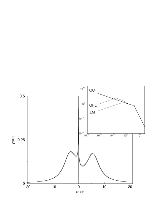
Figure 16: Single-particle dynamics close to and at the QCP, for $r=0.3$ and $\eta=0.2$. Inset: $\pi D(\omega)$ vs $|\omega|$ for $\omega>0$ on a logarithmic scale, for $U=12.0$ (GFL), $12.4$ (LM) and $12.2$ (QCP). The main figure shows the corresponding spectra vs $\omega$ on a linear scale. Full discussion in text.

As $U\rightarrow U_{\mbox{\scriptsize{c}}}(r,\eta)\pm$ and the low-energy scale $\omega_{*}\rightarrow 0$, this $|\omega|^{-r}$ power law persists to lower and lower frequencies, and alone survives at the QCP where $\omega_{*}=0$ identically and the low-energy physics is scale-free. The LMA enables a direct determination of the spectrum precisely at the QCP $U=U_{\mbox{\scriptsize{c}}}(r,\eta)$ (numerically in general, and analytically for small $r$ as in §7). The resultant QCP spectrum for $r=0.3,\eta=0.2$ is also shown in figure; from which the characteristic behaviour $\pi D(U_{\mbox{\scriptsize{c}}};\omega)=C(r,\eta)|\omega|^{-r}$ as $|\omega|\rightarrow 0$ is clearly seen (and which in fact persists essentially up to non-universal scales $\omega\sim{\cal{O}}(1)$).

One obvious but important point should also be noted from the above discussion: close to the transition, and in either phase, $\omega_{*}$ acts as the natural crossover frequency scale to the emergence of common QCP behaviour for $|\omega|\gg\omega_{*}$ in single-particle dynamics, while for lower energies the spectral characteristics are particular to the phase considered. This is of course the dynamical analogue, at $T=0$, of the common schematic pertaining to static/thermodynamic properties at finite-$T$ (see e.g. [21] or figure 1 of [19]), showing the crossover to QCP behaviour upon increasing $T$ above $T\sim\omega_{*}$.

6.4 Scaling: a closer look

In the preceding sections we have focussed primarily on the asymmetric PAIM, $\eta\neq 0$. The purpose of this section is three-fold. First, to compare results for $\eta\neq 0$ to those arising in the particle-hole symmetric limit $\eta=0$ [15,16,20]. There are of course important differences between the two — notably that for $\eta=0$ the LM phase alone arises for all $r>\frac{1}{2}$ and any $U\neq 0$ [10-20] — but, that aside, these are not as radical as might perhaps be inferred from the literature and the two may be readily understood on a common footing.

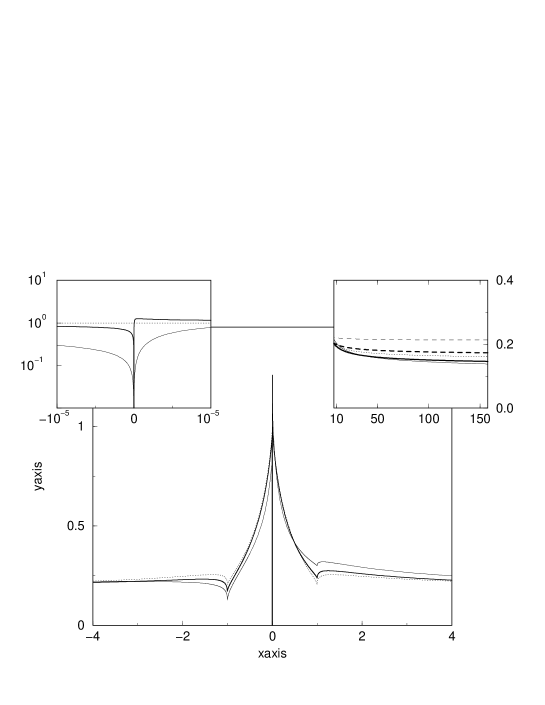
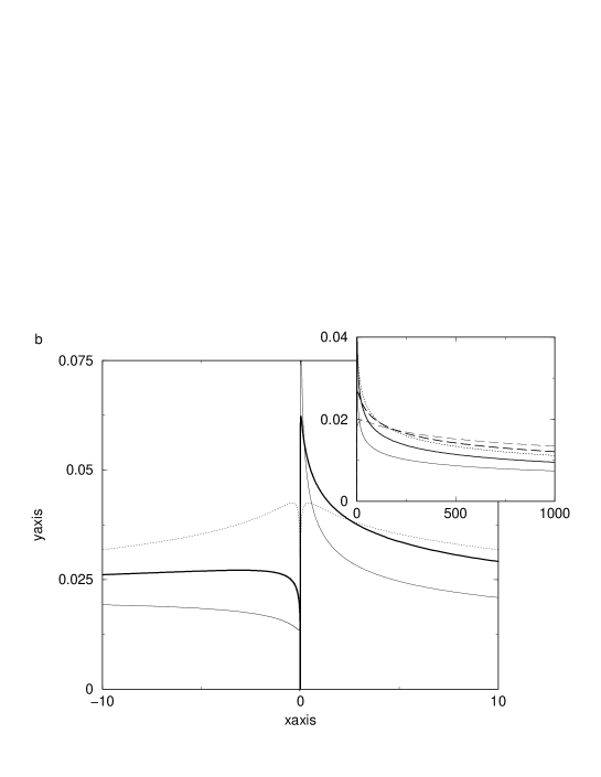
Figure 17: Scaling spectra in both phases for fixed $r$ ($=0.3$) and varying asymmetry $\eta$. A (upper): GFL phase scaling spectrum ${\cal{F}}(\omega)=$sec${}^{2}(\frac{\pi}{2}r)|\tilde{\omega}|^{r}\times\pi\omega_{*}^{r}D(\omega)$ vs $\tilde{\omega}=\omega/\omega_{*}$ ($\omega_{*}\equiv\omega_{\mbox{\scriptsize{m}}}$) for asymmetries $\eta=0$ (dotted line), 0.2 (bold solid) and $0.5$ (thin solid line). The main figure shows the central ‘Kondo resonance’. The right inset shows the spectral ‘tails’ out to $|\tilde{\omega}|=150$, $\eta=0$ (dotted line), $\eta=0.2$ (bold solid line for $\omega>0$, bold dashed line for $\omega<0$) and $\eta=0.5$ (thin solid [dashed] line for $\omega>0$ [$\omega<0$]). Left inset: scaling spectra for $\eta=0,0.2$ and $0.5$ on the lowest scales (cf figure 11). B (lower): LM phase scaling spectrum $\pi\omega_{*}^{r}D(\omega)$ vs $\tilde{\omega}=\omega/\omega_{*}$ ($\omega_{*}\equiv\omega_{\mbox{\scriptsize{L}}}$) for $\eta=0$ (dotted line), $\eta=0.2$ (bold solid line) and $\eta=0.5$ (thin solid line). Inset: spectra shown out to $|\tilde{\omega}|=10^{3}$ for both $\tilde{\omega}>0$ and $<0$, same labelling as in figure 17A.

In comparing dynamics for $\eta\neq 0$ and $\eta=0$, an obvious but important point should first be noted: that we have considered the scaling spectra in terms of $\tilde{\omega}=\omega/\omega_{*}$ and that the low-energy scale $\omega_{*}$ is non-vanishing throughout both phases, including the particle-hole symmetric limit $\eta=0$ [15,20]. In the GFL phase for example one might have chosen, as in §6.1, to express scaling in terms of $\omega/T^{*}$; with $T^{*}\propto|\epsilon_{\mbox{\scriptsize{i}}}^{*}|^{\frac{1}{r}}$ given by equation (6.4) such that the low-energy maxima in the GFL phase spectra lie at $\omega/T^{*}=\pm 1$. This is the procedure adopted in [18] and — in general — is entirely equivalent to ($\omega/\omega_{*}$)-scaling because $T^{*}\propto\omega_{*}$. But the proportionality between the two, given (see equation (3.11)) from $k(r,\eta)=\frac{|\epsilon_{\mbox{\scriptsize{i}}}^{*}|}{\omega_{*}^{r}}\sim(\frac{T^{*}}{\omega_{*}})^{r}$ is odd in $\eta$, such that $\epsilon_{\mbox{\scriptsize{i}}}^{*}$ vanishes throughout the GFL phase in the symmetric limit, while $\omega_{*}\equiv\omega_{\mbox{\scriptsize{m}}}$ remains non-zero. For this reason, scaling in terms of $\omega_{*}$ is naturally required to consider the symmetric and asymmetric PAIMs on an equivalent footing.

In comparing the GFL phase scaling spectra for different $\eta$, it is also convenient to consider the so-called modified spectral function [14-16,20] ${\cal{F}}(\omega)=$sec${}^{2}(\mbox{$\frac{\pi}{2}$}r)\pi|\omega|^{r}D(\omega)$, i.e.

$${\cal{F}}(\omega)=sec^{2}(\mbox{$\frac{\pi}{2}$})r)|\tilde{\omega}|^{r}\times\pi\omega_{*}^{r}D(\omega)$$ (6.7)

(likewise universally dependent on $\tilde{\omega}$). For $\eta=0$ the resultant spectrum is ‘pinned’ at the Fermi level for all $U$ in the GFL phase [14-16], ${\cal{F}}(\omega=0)=1$ (as follows from equation (3.5)); while for any $\eta\neq 0$, ${\cal{F}}(\omega)\propto|\tilde{\omega}|^{2r}$ as $|\tilde{\omega}|\rightarrow 0$. The scale on which this distinction between the $\eta=0$ and $\eta\neq 0$ scaling spectra arises is $T^{*}$ ($\propto\omega_{*})$ as discussed in §6.1 (figure 11). But in practice the ratio $T^{*}/\omega_{*}$ is found within the LMA to be small ($T^{*}/\omega_{*}\sim[k(r,\eta]^{\frac{1}{r}}$ with $k$ itself small compared to unity), so the qualitative differences between $\eta=0$ and $\neq 0$ are apparent only on the lowest-$\tilde{\omega}$ scales. This is seen clearly in the left inset to figure 17a which, for $r=0.3$ and asymmetries $\eta=0,0.2$ and $0.5$, shows ${\cal{F}}(\omega)$ vs $\tilde{\omega}$ for $|\tilde{\omega}|\ll 1$.

By contrast however, the strong similarities between particle-hole symmetric and asymmetric spectra in the GFL phase are also evident in figure 17a. The main figure gives ${\cal{F}}(\omega)$ on the $|\tilde{\omega}|\sim{\cal{O}}(1)$ scale, showing clearly the low-energy ‘Kondo resonance’ in ${\cal{F}}(\omega)$ [14-16] (which becomes precisely the usual Kondo resonance of the metallic AIM in the $r=0$ limit [14-16]). The effects of non-zero $\eta$, while present, do not lead to qualitatively different behaviour either on the $\tilde{\omega}\sim{\cal{O}}(1)$ scales or in the spectral ‘tails’, shown out to $\tilde{\omega}\sim{\cal{O}}(10^{2})$ in the right inset. These comments hold also for the LM phase scaling spectra, $\pi\omega_{\mbox{\scriptsize{L}}}^{r}D(\omega)$ vs $\tilde{\omega}=\omega/\omega_{\mbox{\scriptsize{L}}}$ being shown in figure 17b (again for $r=0.3$ and $\eta=0,0.2$ and $0.5$). In this case $\pi\omega_{\mbox{\scriptsize{L}}}^{r}D(\omega)\propto|\tilde{\omega}|^{r}$ as $\tilde{\omega}\rightarrow 0$ for both the symmetric and asymmetric cases. The spectra for different $\eta$ are thus qualitatively similar for all $\tilde{\omega}$, albeit that the extent of spectral asymmetry naturally increases with $\eta$.

In previous sections we have emphasised in particular the crossover from the $\propto|\tilde{\omega}|^{r}$ behaviour of $\pi\omega_{*}^{r}D(\omega)$ arising at low-$\tilde{\omega}$ to the ultimate large-$\tilde{\omega}$ behaviour $\propto|\tilde{\omega}|^{-r}$ that in turn controls the QCP spectrum. Our second point is simply to note that for the GFL phase, the asymptotic approach to the ultimate $|\tilde{\omega}|^{-r}$ form — where the corresponding ${\cal{F}}(\omega)\propto|\tilde{\omega}|^{r}\times\omega_{*}^{r}D(\omega)$ thus plateaus to a constant — is quite subtle. In figure 17a for example, where the spectral tails of ${\cal{F}}(\omega)$ are shown out to $|\tilde{\omega}|=150$, ${\cal{F}}(\omega)$ has not yet reached its plateau value but is still decreasing, albeit slowly; indeed from figure 12 it is clear the plateau does not occur until $\tilde{\omega}\sim{\cal{O}}(10^{3})$ for the case of $r=0.3$ shown. The approach to the ultimate large-$\tilde{\omega}$ behaviour of the scaling spectrum is thus slow, and in fact becomes progessively more so with diminishing $r\rightarrow 0$. The nature of this behaviour (which is relevant to the GFL phase alone) is known from our recent work on the symmetric PAIM [20] and is modified only quantitatively for $\eta\neq 0$: as $r\rightarrow 0$, the ultimate large-$|\tilde{\omega}|$ behaviour arises only for $|\tilde{\omega}|\gg e^{\frac{1}{r}}$. For $1\ll|\tilde{\omega}|\ll e^{\frac{1}{r}}$ by contrast the decay of ${\cal{F}}(\omega)$ towards its plateau value is logarithmically slow. This ‘intermediate’ large-$\tilde{\omega}$ regime progressively dominates the GFL scaling spectrum out to ever larger-$\tilde{\omega}$ scales as $r\rightarrow 0$, and for $r=0$ recovers precisely the known [26] logarithmic large-$\tilde{\omega}$ tails characteristic of the metallic AIM (for which $D(\omega)\propto 1/ln^{2}(|\tilde{\omega}|)$ for $|\tilde{\omega}|\gg 1$). While it is the small-$r$ behaviour to which we turn in the final section, the reader is referred to [20] for further details on this point.

As noted above, the ultimate large-$\tilde{\omega}$ behaviour $\omega_{*}^{r}D(\omega)\propto|\tilde{\omega}|^{-r}$ is not in fact reached in the $\tilde{\omega}$-range shown in figure 17a for the GFL phase. In consequence none of the behaviour illustrated in the figure survives at the QCP itself. Our final remark here is simply to emphasise this point, evident also in figure 16 (inset): the Kondo resonance in ${\cal{F}}(\omega)$, illustrated clearly figure 17a and characteristic of the GFL phase, ‘collapses’ at the QCP where its weight vanishes; as indeed remarked in [19], and which the above figures substantiate.

7 Small $r$ asymptotics

Our aim now is to obtain analytical results for the critical behaviour of the low-energy scales $\omega_{*}$, the phase boundaries and single-particle scaling spectra, in the strong coupling regime where $U_{\mbox{\scriptsize{c}}}(r,\eta)\gg 1$. This means in effect that we consider here small $r\ll 1$, since $U_{\mbox{\scriptsize{c}}}^{-1}\propto r$ as $r\rightarrow 0$ (see e.g. figure 8).

In strong coupling, where the impurity charge $n\rightarrow 1$, the low-energy behaviour of the pseudogap AIM maps under a Schrieffer-Wolff transformation onto the corresponding Kondo model [2], with host density of states $\rho_{\mbox{\scriptsize{host}}}(\omega)=\rho_{0}|\omega|^{r}\theta(D-|\omega|)$. The exchange coupling matrix element $J=2V^{2}[1/|\epsilon_{\mbox{\scriptsize{i}}}|+1/(U-|\epsilon_{\mbox{\scriptsize{i}}}|)]$, i.e. $J=8V^{2}/[U(1-\eta^{2})]$ expressed in terms of $U$ and $\eta\equiv 1-2|\epsilon_{\mbox{\scriptsize{i}}}|/U$; and the corresponding potential scattering strength is $K=\eta J$. Since the PAIM hybridization $\Delta_{\mbox{\scriptsize{I}}}(\omega)=\pi V^{2}\rho_{\mbox{\scriptsize{host}}}(\omega)$ (with $\Delta_{\mbox{\scriptsize{I}}}(\omega)$ given by equation (2.4)), it follows that

$$\rho_{0}J=\frac{8}{\pi U}\frac{1}{1-\eta^{2}}$$ (7.1)

from which strong coupling PAIM results can be transcribed directly to those applicable to the Kondo model.

As a straightforward generalisation of [15,20] we first focus on $\{\Sigma_{\sigma}(\omega)\}$ in the GFL phase (equation (4.14)), where in strong coupling $\Sigma_{\sigma}(\omega)$ takes the form

$$\Sigma_{\sigma}(\omega)\sim U^{2}{\cal{G}}_{-\sigma}^{-\sigma}(\omega+\sigma\omega_{\mbox{\scriptsize{m}}}).$$ (7.2)

This follows from the fact that the spectral weight of Im$\Pi^{+-}(\omega)$ in strong coupling is confined asymptotically to $\omega>0$ with $\int^{\infty}_{0}(\mbox{d}\omega/\pi)$Im$\Pi^{+-}(\omega)=1$ (which physically reflects saturation of the local moment, $|\mu|\rightarrow 1$); and that its resonance is centred on the low-energy spin-flip scale $\omega_{m}$, on which scales the $\{{\cal{G}}^{\sigma}_{\sigma}(\omega)\}$ are slowly varying. From equation (4.14), equation (7.2) thus results. Equation (7.2) with $\omega_{\mbox{\scriptsize{m}}}=0$ also holds for the LM phase, with $\omega_{\mbox{\scriptsize{m}}}=0$ reflecting as ever the local spin-degeneracy inherent to the LM state; as follows from equation (4.18) noting that [15,20] the LM poleweight $Q\rightarrow 1$ in strong coupling (and that the ${}^{\mbox{\scriptsize{S}}}\Sigma_{\sigma}(\omega)$ contribution is both negligible in intensity and subdominant in frequency [15]).

Re${\cal{G}}^{\sigma}_{\sigma}(\omega)$ is given by the one-sided Hilbert transform equation (4.15), and its leading low-$\omega$ behaviour in strong coupling (and hence for $r\rightarrow 0$) is readily obtained using the methods of [15,20,27]. The result is

$$U^{2}\mbox{Re}{\cal{G}}_{-\sigma}^{-\sigma}(\omega)\sim\sigma\frac{4\lambda^{r}}{\pi r}g_{\sigma}(e_{\mbox{\scriptsize{i}}}^{\prime})\left[1-\frac{|\omega|^{r}}{\lambda^{r}}\right]+{\cal{O}}(|\omega|)$$ (7.3)

where $\lambda=$min$(D,U)$ arises as a high-energy cutoff [15,20,27] and $g_{\sigma}\equiv g_{\sigma}(e_{\mbox{\scriptsize{i}}}^{\prime})=[1+\sigma e_{\mbox{\scriptsize{i}}}^{\prime}]^{-2}$, with $e_{\mbox{\scriptsize{i}}}^{\prime}=2e_{\mbox{\scriptsize{i}}}/U$ and $e_{\mbox{\scriptsize{i}}}$ determined as specified in §s 4.1.1 and 4.3. Equations (7.2) and (7.3) for $\Sigma^{\mbox{\scriptsize{R}}}_{\sigma}(\omega=0)$ will now be employed to determine the critical behaviour of $\omega_{*}\equiv\omega_{\mbox{\scriptsize{m}}}$, and consequent phase boundaries. We also note that the introduction of $\lambda=$min$(D,U)$ means the following analysis encompasses not only $D\gg U$ (as exemplified by the wide band limit $D=\infty$ employed explicitly in the full calculations of previous sections), but in addition the case $U\gg D$. As will be seen, the essential differences between the two naturally reside only in the precise dependence of the low-energy scales and phase boundaries [15,16] on bare model parameters; while for obvious physical reasons the scaling spectra for both phases are entirely independent of whether $D\gg U$ or vice versa.

7.1 Statics: scales and phase boundaries

We consider first the approach to the transition from the GFL phase, determining thereby the critical $U_{\mbox{\scriptsize{c}}}(r,\eta)$ for small-$r$ and the critical behaviour of the Kondo spin-flip scale $\omega_{\mbox{\scriptsize{m}}}\equiv\omega_{*}$ as $U\rightarrow U_{\mbox{\scriptsize{c}}}-$. A brief discussion is then given of resultant phase boundaries, and the corresponding low-energy scale $\omega_{*}\equiv\omega_{\mbox{\scriptsize{L}}}$ characteristic of the LM phase.

The symmetry restoration condition equation (4.5) is a central element of our approach to the GFL phase. Using equation (4.9) it is given in strong coupling (where $|\bar{\mu}|\rightarrow 1$) by $\Sigma^{\mbox{\scriptsize{R}}}_{\uparrow}(0)-\Sigma^{\mbox{\scriptsize{R}}}_{\downarrow}(0)=U$; and hence from equations (7.2,3) by

$$\frac{4\lambda^{r}}{\pi r}\left[1-\left(\frac{\omega_{\mbox{\scriptsize{m}}}}{\lambda}\right)^{r}\right]{\sum_{\sigma}}g_{\sigma}=U.$$ (7.4)

From this the critical $U_{\mbox{\scriptsize{c}}}(r,\eta)$, where $\omega_{\mbox{\scriptsize{m}}}=0$, follows directly from $(\lambda^{r}/U_{\mbox{\scriptsize{c}}}(r,\eta)){\stackrel{{\scriptstyle r\rightarrow 0}}{{\sim}}}(\pi r/4)({\sum_{\sigma}}g_{\sigma})^{-1}$, whence $U_{\mbox{\scriptsize{c}}}^{-1}$ vanishes linearly in $r$ as $r\rightarrow 0$ as noted in the discussion of figure 8 (§5.1). In the particle-hole symmetric ($\eta=0$) limit, $e_{\mbox{\scriptsize{i}}}^{\prime}=0$ (for all $r$ and $U$, see §4) and hence $g_{+}=1=g_{-}$; the result obtained previously in [15] is then recovered, $U_{\mbox{\scriptsize{c}}}^{-1}(r,\eta=0)=\pi r/8$ as $r\rightarrow 0$, which is exact [15,16]. More generally a knowledge of the $g_{\sigma}$ as $r\rightarrow 0$ is required. But since $U_{\mbox{\scriptsize{c}}}^{-1}(r,\eta)\propto r$ as above, the $e_{\mbox{\scriptsize{i}}}^{\prime}$ and hence $g_{\sigma}$ may be replaced asymptotically by their corresponding $r=0$ values [27]; these are $U$-independent and functions solely of the asymmetry $\eta$, given explicitly within the present LMA by [27]

$$g_{\pm}=\frac{f(\eta^{2})}{1\pm\eta}\ \ \ \ :\ \ f(\eta^{2})=\mbox{$\frac{1}{2}$}[1+(1-\eta^{2})^{\frac{1}{2}}].$$ (7.5)

(This result may also be obtained by detailed consideration of the limit $r\rightarrow 0$ itself, analysis of the renormalised level $\epsilon_{\mbox{\scriptsize{i}}}^{*}\equiv\epsilon_{\mbox{\scriptsize{i}}}+\tilde{\Sigma}^{\mbox{\scriptsize{R}}}_{\sigma}(0)$ showing both that the $g_{\sigma}$ given above hold as $U\rightarrow U_{\mbox{\scriptsize{c}}}(r,\eta)$ and that the exponent for the vanishing of $|\epsilon_{\mbox{\scriptsize{i}}}^{*}|\sim u^{a_{1}}$ (equation (3.10)) is indeed $a_{1}=1$ as in figure 4.) From equations (7.4,5) the critical $U_{\mbox{\scriptsize{c}}}(r,\eta)$ is thus given from

$$\frac{\lambda^{r}}{U_{\mbox{\scriptsize{c}}}(r,\eta)}\stackrel{{\scriptstyle r\rightarrow 0}}{{\sim}}\frac{\pi r}{8}\frac{(1-\eta^{2})}{f(\eta^{2})}$$ (7.6)

or equivalently

$$f(\eta^{2})\rho_{0}J_{\mbox{\scriptsize{c}}}\stackrel{{\scriptstyle r\rightarrow 0}}{{\sim}}\frac{r}{\lambda^{r}}$$ (7.7)

for the critical exchange coupling of the corresponding Kondo model.

We shall return to this below, but note first that the $U\rightarrow U_{\mbox{\scriptsize{c}}}(r,\eta)-$ critical behaviour of the Kondo scale $\omega_{\mbox{\scriptsize{m}}}$ follows in turn from equation (7.4) as

$$\frac{\omega_{\mbox{\scriptsize{m}}}}{\lambda}\sim\left(1-{\frac{U}{U_{\mbox{\scriptsize{c}}}(r,\eta)}}\right)^{\frac{1}{r}}.$$ (7.8)

The exponent for the vanishing of the low-energy GFL scale $\omega_{\mbox{\scriptsize{m}}}\equiv\omega_{*}$ is thus $1/r$; as found in figure 3 where, with $\lambda=$min$(D,U)\equiv U$ as appropriate to the wide band limit $D=\infty$ there employed, $(\omega_{*}/U)^{r}$ vs $U$ was shown to vanish linearly in $u=(1-U/U_{\mbox{\scriptsize{c}}})$ as $u\rightarrow 0+$. We add moreover that using equation (7.6) in equation (7.8) and taking the limit $r\rightarrow 0$ recovers precisely the Kondo scale hitherto found in [27] for the $r=0$ metallic AIM,

$$\frac{\omega_{\mbox{\scriptsize{m}}}(r=0)}{\lambda}=exp\left(-\frac{\pi U}{8}\frac{(1-\eta^{2})}{f(\eta^{2})}\right)\equiv exp\left(-\frac{1}{\rho_{0}J}\frac{1}{f(\eta^{2})}\right)$$ (7.9)

(with $J\equiv J(U,\eta^{2})$ given by equation (7.1)). While recovery of an exponentially small Kondo scale from an approximate theory is non-trivial, we note that the exponent therein differs in general from the exact result [2] for the $r=0$ Kondo model by the factor of $f(\eta^{2})\in[1,\frac{1}{2}]$. It is thus as such exact only for the symmetric model where $f(\eta=0)=1$; albeit that the correction is modest, $f$ being slowly varying in $\eta$ and lying e.g. within $10\%$ of unity for $\eta<0.6$. Since equation (7.6) (or equivalently equation (7.7)) likewise reflects the $r=0$ exponent, the $\eta$-dependence of the corresponding exact result as $r\rightarrow 0$ is obtained by replacing $f(\eta^{2})$ by $1$ therein.

The $r\rightarrow 0$ phase boundary arising from equation (7.6) is shown in figure 6 of §5.2 (with $\lambda\equiv U$ as appropriate to the wide-band limit), where it is compared to full numerical results for $r=0.2$ and displayed as $\eta$ vs $(8/\pi r)U^{r-1}_{\mbox{\scriptsize{c}}}(r,\eta)$ — which we note is equivalently lim${}_{r\rightarrow 0}[U_{\mbox{\scriptsize{c}}}(r,\eta=0)/U_{\mbox{\scriptsize{c}}}(r,\eta)]$. Here we add in passing that the resultant $r\rightarrow 0$ phase boundary between non-magnetic (GFL) and magnetic (LM) states, is redolent of the phase diagram obtained in Anderson’s original paper on the $r=0$ metallic AIM (figure 4 of [1]). There is of course no transition for $r=0$: the ‘phase diagram’ of [1] was simply the boundary to local moment formation at MF level, the qualitative deficiencies of which are long since known; in particular that a spurious transition arises at a critical $U^{\mbox{\scriptsize{MF}}}_{\mbox{\scriptsize{c}}}(r=0,\eta)$ (with $U^{\mbox{\scriptsize{MF}}}_{\mbox{\scriptsize{c}}}(0,0)=\pi$). But the similarities between the two are nonetheless striking and the $r=0$ MF results for $\eta$ vs $[U^{\mbox{\scriptsize{MF}}}_{\mbox{\scriptsize{c}}}(0,\eta=0)/U^{\mbox{\scriptsize{MF}}}_{\mbox{\scriptsize{c}}}(0,\eta)]$ ([1], figure 4), while wrong for $r=0$ itself, appear ironically to be qualitatively correct as $r\rightarrow 0$.

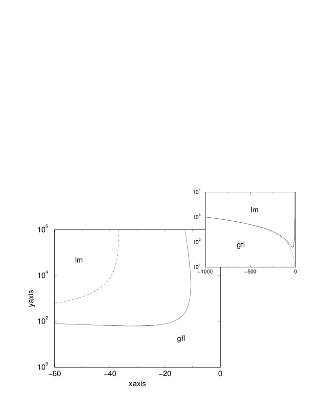
Figure 18: Phase boundary in the $(U,\epsilon_{\mbox{\scriptsize{i}}})$-plane for fixed $r=0.05$ (solid line), obtained from equation (7.6) (with $\lambda=U$ as appropriate to the wide band case). The corresponding result for $r=0.01$ is shown for comparison (dashed line). Inset: $r=0.05$ phase boundary for large negative $\epsilon_{\mbox{\scriptsize{i}}}$, which is seen to approach asymptotically $U_{\mbox{\scriptsize{c}}}=|\epsilon_{\mbox{\scriptsize{i}}}|+$.

Figure 18 by contrast shows the phase diagram in the ($U,\epsilon_{\mbox{\scriptsize{i}}}$)-plane arising from equation (7.6) (with $\lambda=U$), for both $r=0.05$ (solid line) and $r=0.01$; the former showing again the re-entrant behaviour discussed in §5.2 in connection with figure 5. The increasing stability of the GFL phase with diminishing $r$ is clearly evident, and expected physically since the Fermi liquid phase alone persists throughout the entire $(U,\epsilon_{\mbox{\scriptsize{i}}})$-plane in the $r=0$ limit of the metallic AIM. The inset to the figure also shows the phase boundary (for $r=0.05$) out to large negative $\epsilon_{\mbox{\scriptsize{i}}}$, from which it is seen that the critical $U_{\mbox{\scriptsize{c}}}$ asymptotically approaches $|\epsilon_{\mbox{\scriptsize{i}}}|+$ (shown as a dotted line) — again physically natural, this being the condition for local moment formation in the atomic limit.

In figure 19 the $r$-dependence of full LMA phase boundaries is shown for a range of asymmetries $\eta$, and the wide-band limit employed in previous sections. Specifically, $F(r,\eta)=(8/\pi)[f(\eta^{2})/(1-\eta^{2})]U_{\mbox{\scriptsize{c}}}^{r-1}(r,\eta)$ vs $r$ is shown, which from equation (7.6) should behave as $F(r,\eta)\sim r$ as $r\rightarrow 0$ such that phase boundaries for different $r$ then collapse to a common curve. This behaviour is indeed seen in figure 19 and we note that, in line with results from a previous NRG study [13], the resultant phase boundaries have little asymmetry dependence up to $r\simeq 0.25$. The asymptotic behaviour $F(r,\eta)\sim r$ is also shown on the figure and seen to be reached in practice below $r\sim 0.1$ or so (which range we add is known from a previous LMA and NRG study [16] of the symmetric limit to be enhanced further if one works instead with a finite bandwith $D$, with $U/D\gg 1$).

Figure 19: Full LMA phase boundaries, shown as $F(r,\eta)\equiv(8/\pi)[f(\eta^{2})/(1-\eta^{2})]U^{r-1}$ vs $r$, for different asymmetries $\eta=0.1$, 0.2, 0.3, 0.4 and $0.5$ (from top to bottom in sequence). As $r\rightarrow 0$, all collapse to the common form $F(r,\eta)\sim r$ (itself shown, dashed line).

We now consider briefly the corresponding $U\rightarrow U_{\mbox{\scriptsize{c}}}+$ critical behaviour of the low-energy scale $\omega_{*}\equiv\omega_{\mbox{\scriptsize{L}}}$ characteristic of the LM phase, given by equation (6.6) (the resultant phase boundary $U_{\mbox{\scriptsize{c}}}(r,\eta)$ is of course correctly independent of the phase from which it is approached). This is straightforward, since in strong coupling (where $|\bar{\mu}|\rightarrow 1$), $\tilde{\Sigma}^{\mbox{\scriptsize{R}}}_{\uparrow}(0)-\tilde{\Sigma}^{\mbox{\scriptsize{R}}}_{\downarrow}(0)=\Sigma_{\uparrow}^{\mbox{\scriptsize{R}}}(0)-\Sigma_{\downarrow}^{\mbox{\scriptsize{R}}}(0)-U$ from equation (4.9); and $\Sigma_{\sigma}^{\mbox{\scriptsize{R}}}(0)$ is given from equations (7.2,3) with $\omega_{\mbox{\scriptsize{m}}}=0$ throughout the LM phase, whence $\tilde{\Sigma}^{\mbox{\scriptsize{R}}}_{\uparrow}(0)-\tilde{\Sigma}^{\mbox{\scriptsize{R}}}_{\downarrow}(0)=(4\lambda^{r}/\pi r)\sum_{\sigma}g_{\sigma}-U$. But from equation (7.4) $(4\lambda^{r}/\pi r)\sum_{\sigma}g_{\sigma}=U_{\mbox{\scriptsize{c}}}$, so $\tilde{\Sigma}^{\mbox{\scriptsize{R}}}_{\uparrow}(0)-\tilde{\Sigma}^{\mbox{\scriptsize{R}}}_{\downarrow}(0)\sim-U_{\mbox{\scriptsize{c}}}(U/U_{\mbox{\scriptsize{c}}}-1)$ as $U\rightarrow U_{\mbox{\scriptsize{c}}}+$, with $U_{\mbox{\scriptsize{c}}}\propto 1/r$ as $r\rightarrow 0$ from equation (7.6). Hence $\omega_{\mbox{\scriptsize{L}}}\propto(r|\tilde{\Sigma}^{\mbox{\scriptsize{R}}}_{\uparrow}(0)-\tilde{\Sigma}^{\mbox{\scriptsize{R}}}_{\downarrow}(0)|)^{1/r}$ given by equation (6.6) indeed has the critical behaviour

$$\omega_{\mbox{\scriptsize{L}}}\propto\left(\frac{U}{U_{\mbox{\scriptsize{c}}}(r,\eta)}-1\right)^{\frac{1}{r}}$$ (7.10)

with exponent $1/r$, as shown numerically in figure 3 (§5.1).

7.2 Scaling spectra and the QCP

We turn finally to the scaling spectra characteristic of the GFL and LM phases (figures 12, 15), in particular the leading large $\tilde{\omega}=\omega/\omega_{*}$ behaviour thereof that determines the spectrum at the quantum critical point itself (§6.3).

The impurity Green function is given by equations (2.9,10), which may be expressed quite generally as $G(\omega)=\mbox{$\frac{1}{2}$}\sum_{\sigma}[\omega^{+}-\Delta(\omega)-\epsilon_{\mbox{\scriptsize{i}}\sigma}^{*}-(\Sigma_{\sigma}(\omega)-\Sigma_{\sigma}(0))]^{-1}$, where we use $\tilde{\Sigma}_{\sigma}(\omega)-\tilde{\Sigma}_{\sigma}(0)=\Sigma_{\sigma}(\omega)-\Sigma_{\sigma}(0)$ (trivially, from equation (4.9)). Here as usual, $\epsilon_{\mbox{\scriptsize{i}}\sigma}^{*}=\epsilon_{\mbox{\scriptsize{i}}}+\tilde{\Sigma}_{\sigma}(0)$ is the renormalised level (equation (5.20)); with the $\epsilon_{\mbox{\scriptsize{i}}\sigma}^{*}=\epsilon_{\mbox{\scriptsize{i}}}^{*}$ independent of spin $\sigma$ for the GFL phase where symmetry is restored (equation (4.5)), but $\epsilon_{\uparrow}^{*}\neq\epsilon_{\downarrow}^{*}$ for the LM phase, as shown in §5.1. As discussed in the preceding sections, (i) the scaling spectra for the GFL or LM phases are obtained by considering finite $\tilde{\omega}=\omega/\omega_{*}$ (with $\omega_{*}=\omega_{\mbox{\scriptsize{m}}}$ or $\omega_{\mbox{\scriptsize{L}}}$ as appropriate), in the formal limit $\omega_{*}\rightarrow 0$; and (ii) it is $\omega_{*}^{r}G(\omega)$ (as opposed to $G(\omega)$ itself) which exhibits universal scaling in terms of $\tilde{\omega}$. This follows directly, $\omega_{*}^{r}G(\omega)=\mbox{$\frac{1}{2}$}\sum_{\sigma}[\omega_{*}^{1-r}\tilde{\omega}^{+}-\omega_{*}^{-r}\Delta(\omega)-\omega_{*}^{-r}(\epsilon_{\mbox{\scriptsize{i}}\sigma}^{*}+(\Sigma_{\sigma}(\omega)-\Sigma_{\sigma}(0))]^{-1}$, in which $\omega_{*}^{1-r}|\tilde{\omega}|$ may be neglected entirely for $0\leq r<1$ as considered. By contrast, from equations (2.4,5) for the hybridization, $\omega_{*}^{-r}\Delta(\omega)$ is non-vanishing in the scaling regime and given by $\omega_{*}^{-r}\Delta(\omega)=-$sgn$(\omega)[\beta(r)+\mbox{i}]|\tilde{\omega}|^{r}$ (independently of the bandwith $D$). The scaling spectrum $\pi\omega_{*}^{r}D(\omega)=-$sgn$(\omega)\omega_{*}^{r}$Im$G(\omega)$ is thus obtained from

$$\omega_{*}^{r}G(\omega)={\mbox{$\frac{1}{2}$}}{\sum_{\sigma}}\left[\mbox{sgn}(\omega)[\beta(r)+\mbox{i}]|\tilde{\omega}|^{r}-\frac{\epsilon_{\mbox{\scriptsize{i}}\sigma}^{*}}{\omega_{*}^{r}}-\omega_{*}^{-r}(\Sigma_{\sigma}(\omega)-\Sigma_{\sigma}(0))\right]^{-1}$$ (7.11)

which we add holds generally for all $0\leq r<1$ considered; and where $\epsilon_{\mbox{\scriptsize{i}}\sigma}^{*}/\omega_{*}^{r}$ as $\omega_{*}\rightarrow 0$ has been shown in §5.1 to tend to a non-zero constant for both the GFL and LM phases (denoted therein as $k(r,\eta)$ for the GFL phase).

Since $\omega_{*}^{r}G(\omega)$ scales, it follows from equation (7.11) that $\omega_{*}^{-r}[\Sigma_{\sigma}(\omega)-\Sigma_{\sigma}(0)]$ is likewise universally dependent solely on $\tilde{\omega}=\omega/\omega_{*}$. In the strong coupling, $r\rightarrow 0$ regime of interest here, this may be shown directly using equations (7.2,3) (together for $\Sigma^{\mbox{\scriptsize{I}}}_{\sigma}(\omega)$ with Im${\cal{G}}_{\sigma}^{\pm}(\omega)=-$sgn$(\omega)\pi D_{\sigma}^{0}(\omega)\theta(\pm\omega)$ with $D_{\sigma}^{0}(\omega)$ the MF spectral density). For the GFL phase one thereby finds

$$\omega_{*}^{-r}[\Sigma^{\mbox{\scriptsize{R}}}_{\sigma}(\omega)-\Sigma^{\mbox{\scriptsize{R}}}_{\sigma}(0)]=-\sigma{\frac{4}{\pi r}g_{\sigma}}\ \left[|\tilde{\omega}+\sigma|^{r}-1\right]$$ (7.12a)

$$\omega_{*}^{-r}\Sigma^{\mbox{\scriptsize{I}}}_{\sigma}(\omega)=4g_{\sigma}\ \theta(-[1+\sigma\tilde{\omega}])|\tilde{\omega}+\sigma|^{r}$$ (7.12b)

(noting that $\Sigma^{\mbox{\scriptsize{I}}}_{\sigma}(0)=0$); where the $g_{\sigma}\equiv g_{\sigma}(\eta)$ are given explicitly by equation (7.5) and $\omega_{*}\equiv\omega_{\mbox{\scriptsize{m}}}$. For the LM phase by contrast,

$$\omega_{*}^{-r}[\Sigma^{\mbox{\scriptsize{R}}}_{\sigma}(\omega)-\Sigma^{\mbox{\scriptsize{R}}}_{\sigma}(0)]=-\sigma{\frac{4}{\pi r}}g_{\sigma}\ |\tilde{\omega}|^{r}$$ (7.13a)

$$\omega_{*}^{-r}\Sigma^{\mbox{\scriptsize{I}}}_{\sigma}(\omega)=4g_{\sigma}\ \theta(-\sigma\tilde{\omega})|\tilde{\omega}|^{r}$$ (7.13b)

with $\omega_{*}\equiv\omega_{\mbox{\scriptsize{L}}}$. Equations (7.12,13), which we emphasise hold for all $\tilde{\omega}$ (and $r\rightarrow 0$), are indeed of the required universal form; and for $\eta=0$, where the $g_{\sigma}=1$, reduce to the results of [20] for the symmetric PAIM. Together with equation (7.11) they determine the full $\tilde{\omega}$-dependence of the scaling spectra for the respective phases. The resultant range of behaviour is rich, encompassing for example the intermediate logarithmic regime in the GFL phase mentioned in §6.4, and may again be obtained following the arguments of [20].

Here we consider solely the ultimate large-$\tilde{\omega}$ behaviour of the scaling spectra for either phase, relevant to the QCP itself. This arises for $|\tilde{\omega}|^{r}\gg 1$, and for $r\rightarrow 0$ (where $\beta(r)=$tan$(\frac{\pi}{2}r)\sim 0$) equations (7.11–13) yield the requisite behaviour

$$\pi\omega_{*}^{r}D(\omega)\ \stackrel{{\scriptstyle\tilde{\omega}^{r}\gg 1}}{{\sim}}\ \frac{\pi^{2}r^{2}}{32}\left(\frac{1}{g_{+}^{2}}+\frac{1+4g_{-}}{g_{-}^{2}}\right)\ |\tilde{\omega}|^{-r}\ \equiv\ C(r,\eta)|\tilde{\omega}|^{-r}$$ (7.14)

given explicitly for positive $\tilde{\omega}$ (for $\tilde{\omega}<0$, $g_{+}$ and $g_{-}$ are simply interchanged). The result equation (7.14) applies to both the GFL and LM phases; and $\omega_{*}^{r}$ cancels out of each side of the equation to give the behaviour $\pi D(\omega)=C(r,\eta)|\omega|^{-r}$ precisely at the QCP (which in that case extends down to $\omega=0$ (§6.3)). As found numerically the QCP coefficient $C(r,\eta)$ is indeed both $r$- and $\eta$-dependent; with $C(r,\eta)\sim r^{2}$ as $r\rightarrow 0$ and as such from equation (7.6) proportional to $1/[U_{\mbox{\scriptsize{c}}}(r,\eta)]^{2}$ (or equivalently $[\rho_{0}J_{\mbox{\scriptsize{c}}}]^{2}$), in which the interacting nature of the QCP is directly manifest.

8 Summary

We have developed in this paper a non-perturbative local moment approach to the $T=0$ pseudogap Anderson impurity model, with a conduction electron density of states proportional to $|\omega|^{r}$ and itself a longstanding paradigm [6-20] for understanding the topical and important issue of local quantum phase transitions. The transition here is between a generalised fermi liquid phase, perturbatively connected to the non-interacting limit, in which the impurity spectrum exhibits a Kondo-like resonance indicative of underlying local singlet behaviour; and a doubly degenerate local moment phase in which the impurity spin remains unquenched. In addition to phase boundaries, and associated critical behaviour of relevant low-energy scales, local single-particle dynamics in the immediate vicinity of the transition have been considered: in the GFL and LM phases separately, and at the quantum critical point itself where the Kondo resonance has just collapsed and the problem is scale-free. Notwithstanding the range of vanishing low-energy scales as the transition is approached, and their importance in understanding local spectra, dynamics close to the QCP in either phase are nonetheless controlled by a single low-energy scale $\omega_{*}$ and as such scale universally in terms of $\omega/\omega_{*}$. A determination and understanding of these scaling dynamics on all $\omega/\omega_{*}$ scales, including their continuous evolution ‘from the tails’ to pure QCP behaviour, has been a primary focus of the work. Approximate though it is the LMA is to our knowledge one of the few theoretical approaches currently capable of handling these issues; and the description arising from it is both rich and arguably a good deal more subtle than appears to have been appreciated hitherto. Much of course remains to be understood, not least the question of dynamics at finite-temperature, aspects of which will be considered in a forthcoming paper.

References

References

- [1] Anderson P W 1961 Phys. Rev. 124 41
- [2] Hewson A C 1993 The Kondo Problem to Heavy Fermions (Cambridge: Cambridge University Press)
- [3] Goldhaber-Gordon D et al 1998 Nature 391 156
- [4] Cronenwett S M, Oosterkamp T H and Kouwenhoven L P 1998 Science 281 540
- [5] Li J, Schneider W-D, Berndt R and Delley B 1998 Phys. Rev. Lett. 80 2893
- [6] Withoff D and Fradkin E 1990 Phys. Rev. Lett. 64 1835
- [7] Borkovski L S and Hirschfeld P J 1992 Phys. Rev. B 46 9274
- [8] Chen K and Jayaprakash C 1995 J. Phys.: Condens. Matter 7 L491
- [9] Cassanello C R and Fradkin E 1996 Phys. Rev. B 53 15079
- [10] Gonzalez-Buxton C and Ingersent K 1996 Phys. Rev. B 54 15614
- [11] Ingersent K 1996 Phys. Rev. B 54 11936
- [12] Bulla R, Pruschke Th and Hewson A C 1997 J. Phys.: Condens. Matter 9 10463
- [13] Gonzalez-Buxton C and Ingersent K 1998 Phys. Rev. B 57 14254
- [14] Glossop M T and Logan D E 2000 Eur. Phys. J. B 13 513
- [15] Logan D E and Glossop M T 2000 J. Phys.: Condens. Matter 12 985
- [16] Bulla R, Glossop M T, Logan D E and Pruschke T 2000 J. Phys.: Condens. Matter 12 4899
- [17] Vojta M 2001 Phys. Rev. Lett. 87 097202
- [18] Vojta M and Bulla R 2002 Phys. Rev. B 65 014511
- [19] Ingersent K. and Si Q. 2002 Phys. Rev. Lett. 89 076403
- [20] Glossop M T and Logan D E 2003 Europhys. Lett. 61 810
- [21] Sachdev S. 1999 Cambridge: Cambridge University Press
-
[22]
Volkov B A and Pankratov O A 1985 Pis. Zh. Eksp. Teor. Fiz. 42 145
(ENGL. TRANSL. 1985 JETP Lett. 42 178) - [23] Voit J 1995 Rep. Prog. Phys. 58 977
- [24] Si Q., Rabello S., Ingersent K. and Smith J. L. 2001 413 804.
- [25] Logan D E, Eastwood M P and Tusch M A 1998 J. Phys.: Condens. Matter 10 2673
- [26] Dickens N L and Logan D E 2001 J. Phys.: Condens. Matter 13 4505
- [27] Glossop M T and Logan D E 2002 J. Phys.: Condens. Matter 14 6737
- [28] Logan D E and Dickens N L 2002 J. Phys.: Condens. Matter 14 3605
-
[29]
Logan D E and Dickens N L 2001 Europhys. Lett. 54 227
Logan D E and Dickens N L 2001 J. Phys.: Condens. Matter 13 9713 -
[30]
Vidhyadhiraja N S, Smith V E, Logan D E and Krishnamurthy H R
2003 J. Phys.: Condens. Matter 15 40405
Smith V E, Logan D E and Krishnamurthy H R 2003 Eur. Phys. J. B 32 49 - [31] Luttinger J M and Ward J C 1960 Phys. Rev. 118 1417
- [32] Langreth D C 1966 Phys. Rev. 150 516
- [33] Wilson K 1975 Rev. Mod. Phys. 27 773
-
[34]
Keiter H and Kimball J C 1971 Int. J. Magn. 1 233
Bickers N 1987 Rev. Mod. Phys. 59 845
Pruschke T and Grewe N 1989 Z. Phys. 74 439 - [35] Horvatić B, Šokčević D and Zlatić V 1987 Phys. Rev. B 36 675
- [36] Bulla R 2002 Private communication