Inelastically scattering particles and wealth distribution in an open economy

Abstract

Using the analogy with inelastic granular gasses we introduce a model for wealth exchange in society. The dynamics is governed by a kinetic equation, which allows for self-similar solutions. The scaling function has a power-law tail, the exponent being given by a transcendental equation. In the limit of continuous trading, closed form of the wealth distribution is calculated analytically.

I Introduction

The distribution of wealth among individuals within a society was one of the first “natural laws” of economics pareto_1897 . Indeed, its study was motivated by the desire to bring the accuracy attributed to natural sciences, namely physics, to economic sciences. The celebrated Pareto law states that the higher end of the wealth distribution follows a power-law $P(W)\sim W^{-1-\alpha}$ with exponent $\alpha$ robust in time.

The validity of the Pareto law was questioned and re-examined many times but the core message, stating that the tail of the distribution is a power law remains in force. There are recent investigations, e. g. lev_sol_97 ; dra_yak_01a ; ree_hug_02 ; aoy_sou_fuj_03 , giving reasonable empirical evidence for it. In fact, it is not so much the functional form itself but its spatial and temporal stability that is intriguing. Indeed, while the value of the exponent $\alpha$ may slightly vary from one society to another, the very fact of the power-law 0.tail in the distribution is valid almost everywhere. Recent investigations suggest that the range of validity of the Pareto law may extend as far in the past as to the ancient Egypt of the Pharaohs abulmagd_02 .

The universality of the power-law tail is surely a phenomenon asking for explanation. Recently, there was a lot of effort establishing finally the multiplicative random processes repelled from zero as a mathematical source of the power-law distributions lev_sol_96 ; lev_sol_96a ; bi_ma_le_so_98 ; solomon_98 ; solomon_99 ; hua_sol_00 ; sol_ric_01b ; bla_sol_00 ; sol_lev_00 ; hua_sol_01 ; so_co_97 ; sornette_97a ; sornette_98c ; ta_sa_ta_97 . Alternatively, the killed multiplicative processes as sources of power-laws were studied in ree_hug_02 . However, there are plenty of possible ways how the multiplicative random processes of this type come onto scene. One of the most studied implementations were the generalized Lotka-Volterra equations solomon_98 ; solomon_99 ; hua_sol_00 ; sol_ric_01b and the analogy with directed polymers in random media ma_mas_zha_98 ; bou_mez_00 ; bur_joh_jur_kam_nov_pa_zah_01 . Both of these schemes are formalized by a kinetic equation describing the exchange of wealth between agents and global redistribution of wealth which plays the role of repelling from zero. Related approaches were subsequently pursued by a number of studies and simulations souma_00 ; aoy_nag_oka_sou_tak_tak_00 ; souma_02 ; sou_fuj_aoy_01 ; fuj_sou_aoy_kai_aok_02 ; cha_cha_00 ; cha_cha_03 ; cha_cha_man-all ; das_yar_03 ; pia_igl_abr_veg_01 ; igl_gon_pia_veg_abr_03 ; pia_igl_03 ; igl_gon_abr_veg_03 ; ana_ish_suz_tom_03 ; miz_kat_tak_tak_03 ; miz_tak_tak_03 ; fuj_dig_aoy_gal_sou_03 .

More recently, empirical studies of the lower end of the wealth axis showed that the distribution of wealth is rather exponential than power-law, while the high-wealth tail still remains power-law dra_yak_01a ; dra_yak-all ; yakovenko_03 . This finding was interpreted as a result of a conservation law for total wealth, leading to the robust Boltzmann-like exponential distribution, whatever the random wealth exchange be, in full analogy with the energy distribution in a gas of elastically scattering molecules.

This, together with older studies within the same spirit is_kra_re_98 , lead to the view of economic activity as a scattering process of agents, analogous to inelastically scattering particles cha_cha_00 ; cha_cha_03 ; cha_cha_man-all ; sca_pic_wes_02 ; sca_wes_03 ; gli_ign_02 ; sinha_03 . Indeed, the inelasticity is indispensable to explain the power-law tail and it is also reasonable to suppose that the total wealth increases on average.

The numerical simulations performed to date confirm the emergence of power-law tail in agent-scattering processes with great reliability. However, analytic insight is lacking in most of the studies available today. The main concern of our work is to fill this gap, providing analytical results at least for a simplified model of wealth exchange. To comply with the task we will be guided by existing analytical approaches for models of inelastically scattering particles.

Inelastic scattering of particles was studied thoroughly in the context of granular materials ja_na_be_96a . The simplest one of the models used is the Maxwell model, whose inelastic variant was investigated in detail bob_car_gam_00 ; bob_cer-all ; bal_mar_pug_01a ; isp_kra_00 ; benn_kra_00 ; kra_benna_01 ; benn_kra_02a ; bena_benn_lin_ros_03 ; ern_bri_02b ; ern_bri-everything ; benn_kra_03 ; ant_dro_lip_02 ; barkai_03 . More realistic models of granular gasses were also introduced bal_mar_pug_01 ; bal_mar_pug_vul_01 but their full account goes beyond the topic of this work. The most important conclusion of these studies is that a self-similar solution of the kinetic equations exist, which is not stationary in time, but assumes time-independent form after proper rescaling of the energy. The tail of the scaling function becomes power-law under certain condition.

The formalism developed for granular gases can be readily adapted for binary wealth exchange of agents. Indeed, within the mean-field version of the Maxwell model the particles scatter randomly one with another irrespectively of their positions. This corresponds to randomly picking pairs of agents for interaction, with no care of the (possibly complex) structure of their relationships. In reality the economic activity goes along links in a complex social network wa_stro_98 ; bar_alb_99 . Indeed, recently there were investigations of the role of network topology in wealth distribution igl_gon_pia_veg_abr_03 ; dim_ast_hyd_03 . We may consider the present model as an approximation of that network by a complete graph.

The main difference from the mean-field Maxwell model is that the energy of the granular gas decreases by dissipation, while the average total wealth of the agents increases due to the economic activity. The sign of the non-conservation is therefore opposite in the two cases. While the form of the equations may remain the same, the solution cannot be directly continued from one domain to another. Therefore, while the case of dissipation is relatively well understood, new approaches are needed in the case of production. That is the aim of the present work.

II Interacting agents as scattering particles

II.1 Description of the process

Imagine a society of $N$ agents, each of which possess certain wealth $v_{i}$, $i=1,2,...,N$. Time-to time the agents interact in essentially instantaneous “collision” events, when certain fraction of the wealth can be exchanged. Moreover, we suppose the system is open and the interaction can catalyze an increase of the total wealth of the two interacting agents. Indeed, the source of the human wealth lies beyond our society and the ultimate cause is the energy poured to the Earth from the Sun. Nonetheless, the external energy is utilized only through a human activity and we simplify the problem by assuming that the net increase of wealth happens at the very moments of agents’ interaction.

We also assume that only pairwise interaction occurs. This may be a very crude assumption, as corporate decisions affect many agents simultaneously. However, we expect the presence of multilateral interactions does not affect the essential mechanisms in work here.

The dynamics of our model is described as follows. In each time step $t$ a pair of agents $(i,j)$ is chosen randomly. They interact and exchange wealth according to the symmetric rule

$$\left(\begin{array}[]{l}v_{i}(t+1)\\ v_{j}(t+1)\end{array}\right)=\left(\begin{array}[]{cc}1+\epsilon-\beta&\beta\\ \beta&1+\epsilon-\beta\end{array}\right)\left(\begin{array}[]{l}v_{i}(t)\\ v_{j}(t)\end{array}\right)$$ (1)

All other agents leave their wealth unchanged, $v_{k}(t+1)=v_{k}(t)$ for all $k$ different from both $i$ and $j$. The parameter $\beta\in(0,1)$ quantifies the wealth exchanged, while $\epsilon>0$ measures the flow of wealth from the outside. The process is sketched schematically in Fig. 1.

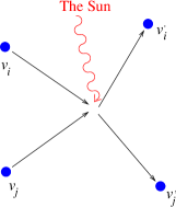
Figure 1: Schematic picture of the scattering process, where the wealth is exchanged and produced.

This rule is similar to those studied in is_kra_re_98 ; benn_kra_00 ; bena_benn_lin_ros_03 and simulated numerically in cha_cha_00 ; cha_cha_man-all ; sca_pic_wes_02 ; sinha_03 but we consider it slightly more realistic as it treats the agents in a priori symmetric manner. It also embraces various sources of wealth non-conservation within a single effective parameter $\epsilon$. In fact, also the formulation based on the similarity with the problem of directed polymers ma_mas_zha_98 ; bou_mez_00 can be reduced to a rule of the form similar to (1). Therefore, we are studying a representative of a whole class of related models and we expect the analytical results we will present have rather broad relevance.

II.2 Kinetic equation

The equation (1) describes a matrix multiplicative stochastic process of vector variable $v(t)$ in discrete time $t$. Processes of this type are thoroughly studied e. g. in the context of granular gasses. Indeed, if the variables $v_{i}$ are interpreted as energies corresponding to $i$-th granular particle, we can map the process to the mean-field limit of the Maxwell model of inelastic particles. However, the energy dissipation conventionally quantified by the restitution coefficient implies now the negative value $\epsilon<0$, contrary to our assumption $\epsilon>0$. We will see later that this apparently small variation makes big difference in the analytical treatment of the process.

The full information about the process in time $t$ is contained in the $N$-particle joint probability distribution $P_{N}(t;v_{1},v_{2},...,v_{N})$. However, we can write a kinetic equation involving only one- and two-particle distribution functions

$$\begin{split}&P_{1}(t+1;v)-P_{1}(t;v)=\frac{2}{N}\bigg{[}-P_{1}(t;v)+\\ &+\int P_{2}(t;v_{i},v_{j})\,\delta((1-\beta+\epsilon)v_{i}+\beta v_{j}-v)\,\mathrm{d}v_{i}\mathrm{d}v_{j}\bigg{]}\end{split}$$ (2)

which may be continued to give eventually an infinite hierarchy of equations of BBGKY type. As a standard approximation we use the factorization

$$P_{2}(t;v_{i},v_{j})=P_{1}(t;v_{i})P_{1}(t;v_{j})$$ (3)

which breaks the hierarchy on the lowest level, neglecting the correlations between the wealth of the agents, induced by the scattering. In fact, this approximation becomes exact for $N\to\infty$. Therefore, in thermodynamic limit the one-particle distribution function bears all information.

Rescaling the time as $\tau=2t/N$ in the thermodynamic limit $N\to\infty$, we obtain for the one-particle distribution function $P(\tau;v)=P_{1}(t,v)$ a Boltzmann-like kinetic equation

$$\begin{split}&\frac{\partial P(v)}{\partial\tau}+P(v)=\\ &\;\int P(v_{i})P(v_{j})\,\delta((1-\beta+\epsilon)v_{i}+\beta v_{j}-v)\,{\rm d}v_{i}{\rm d}v_{j}\end{split}$$ (4)

which describes exactly the process (1) in the limit $N\to\infty$. This equation has the same form as the mean-field version for the well-studied Maxwell model of inelastically scattering particles kra_benna_01 ; bena_benn_lin_ros_03 ; ern_bri_02b . The main difference consists in the fact that here the wealth increases, while in inelastic gas the energy decreases. This seemingly little difference has, however, deep consequences for the solution of Eq. (4).

Note also that within the framework of Maxwell model the distributions are expressed in terms of velocities, while our dynamical variables correspond rather to energies of the particles.

III Solution of the kinetic equation

III.1 Self-similar solutions

Note first that the average wealth $\bar{v}=\int v\,P(v)\,\mathrm{d}v$ in the process described by the kinetic equation (4) grows exponentially

$$\bar{v}(\tau)=\bar{v}(0)\,{\rm e}^{\epsilon\tau}$$ (5)

and therefore Eq. (4) has no stationary solution. However, we may look for a quasi-stationary self-similar solution in the form bob_cer-all ; kra_benna_01 ; bena_benn_lin_ros_03 ; ern_bri_02b

$$P(\tau;v)=\frac{1}{\bar{v}(\tau)}\,\Phi(\frac{v}{\bar{v}(\tau)})\;.$$ (6)

Using the Laplace transform $\hat{\Phi}(x)=\int_{0}^{\infty}\Phi(w)\,{\rm e}^{-xw}\,{\rm d}w$ we can write a non-local differential equation for the scaling function in the form

$$\epsilon x\hat{\Phi}^{\prime}(x)+\hat{\Phi}(x)=\hat{\Phi}((1-\beta+\epsilon)x)\;\hat{\Phi}(\beta x)$$ (7)

A hint about possible solutions can be obtained from a special exactly solvable case $\epsilon=-2\sqrt{\beta}+2\beta$. It can be easily verified kra_benna_01 that the function $\hat{\Phi}_{1}(x)=(1+\sqrt{2x})\mathrm{e}^{-\sqrt{2x}}$ is a solution of (7). Inverting the Laplace transform we obtain the corresponding wealth distribution ${\Phi}_{1}(w)=$ $\frac{1}{\sqrt{2\pi}}$ ${w}^{-5/2}$ $\exp(-\frac{1}{2\,{w}})$ which has similar form as obtained in previous studies sol_ric_01b ; ma_mas_zha_98 ; bou_mez_00 . However, in this case the value of $\epsilon$ is negative, which contradicts our assumption of wealth increase, while for $\epsilon>0$ the above idea leading to the function $\hat{\Phi}_{1}(x)$ does not work. Therefore, we must look for alternative ways. The leading idea of our approach is that equation (7) is nearly local for small values of $\epsilon$ and $\beta$. Therefore, we will expand the factors on the RHS of Eq. (7) in Taylor series in $\epsilon$ and $\beta$ and perform the limit $\epsilon,\beta\to 0$. As the parameters $\epsilon$ and $\beta$ quantify the amount of wealth increase and exchange in single trade event, we interpret the latter limit as the limit of continuous trading. In fact, such limit should involve also a rescaling of time $\tau$, but because we are interested only in stationary regime, the explicit time dependence does not enter our considerations.

It should be also stressed that an important feature can be inferred from the observation that the system behaves differently for positive and negative $\epsilon$. Indeed, it suggests a singularity at the point of precise conservation of wealth, $\epsilon=0$.

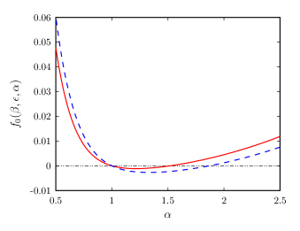
Figure 2: Solution of the equation $f_{0}(\beta,\epsilon,\alpha)\equiv(1+\epsilon-\beta)^{\alpha}+\beta^{\alpha}-1-\epsilon\alpha=0$ for $\epsilon=0.1$ and $\beta=0.0025$ (full line) and $\beta=0.004$ (dashed line).

III.2 Power-law tails

The main concern in empirical studies of wealth distribution is about the shape of tails, which assumes power-law form. The behavior of the distribution $\Phi(w)$ for $w\to\infty$ can be deduced from the singularity of the Laplace transform $\hat{\Phi}(x)$ at $x\to 0$. Therefore, we assume the following behavior kra_benna_01 ; ern_bri_02b

$$\hat{\Phi}(x)=1-x+A\,|x|^{\alpha}+...\text{ for }x\to 0$$ (8)

where $\alpha\in(1,2)$. This type of singularity results in the power-law tail as ${\Phi}(w)\sim w^{-\alpha-1}$ for $w\to\infty$. Insertion of (8) into (7) leads to a transcendental equation for the exponent $\alpha$

$$(1+\varepsilon-\beta)^{\alpha}+\beta^{\alpha}-1-\varepsilon\alpha=0$$ (9)

the solution of which is illustrated in Fig. 2. Obviously, there is always a trivial solution $\alpha=1$. The power-law tail is due to another, non-trivial solution, which falls into the desired interval $(1,2)$ only for certain values of the parameters $\beta$ and $\epsilon$. We can see the allowed region in Fig. 3; solution in the range $\alpha\in(1,2)$ exists within the shaded region. We can also see that fixed value of $\alpha$ defines a line in the $\beta$-$\epsilon$ plane. We can approach the limit $\epsilon\to 0$, $\beta\to 0$ while keeping $\alpha$ constant. This is to be interpreted as continuous trading, as the amount of wealth exchange and increase in a single trading step is infinitesimally small. Making this, the non-local terms in Eq. (7) become local and we can expect to obtain an ordinary differential equation, soluble by standard methods.

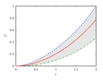
Figure 3: Solution in the range $\alpha\in(1,2)$ exists within the shaded region. dashed line corresponds to $\alpha=2$, dash-dotted line corresponds to $\alpha=1$ and full line to the solution $\alpha=\frac{3}{2}$.

III.3 Continuous trading limit

Indeed, expanding (9) we obtain the following formula relating $\beta$ and $\epsilon$ for fixed $\alpha$ in the limit of continuous trading $\beta\to 0$, $\epsilon\to 0$:

$$\beta=\frac{\alpha-1}{2}\,\epsilon^{2}+O(\epsilon^{3})+O(\epsilon^{2\alpha})\;.$$ (10)

The leading correction term to (10) depends on the value of $\alpha$; for $1<\alpha<3/2$ it is of order $O(\epsilon^{2\alpha})$, for $3/2<\alpha<2$ it is of order $O(\epsilon^{3})$, while in the special point $\alpha=3/2$ we should include both correction terms, as they are of the same order $O(\epsilon^{3})$. Systematic expansion in $\epsilon$ is developed in Appendix A.

Taking the same limit with fixed $\alpha$ in Eq. (7) we obtain, using (10), the following equation

$$-\frac{1}{2}x\hat{\Phi}^{\prime\prime}(x)+\frac{\alpha-1}{2}\left(\hat{\Phi}^{\prime}(x)+\hat{\Phi}(x)\right)=0\;.$$ (11)

Of the two independent solutions of (11) only one has correct asymptotics $\hat{\Phi}(x)\to 0$ for $x\to+\infty$. It can be expressed using modified Bessel function

$$\hat{\Phi}(x)=C^{\prime}\,{x}^{\alpha/2\,}{\it K}_{\alpha}(2\,\sqrt{\alpha-1}\sqrt{x})$$ (12)

where the constant $C^{\prime}$ is fixed by the normalization $\hat{\Phi}(0)=1$. Inverting the Laplace transform we finally obtain the wealth distribution

$$\Phi(w)=C\,{w}^{-\alpha-1}\exp(-\frac{\alpha-1}{w})$$ (13)

with $C=(\alpha-1)^{\alpha}/\Gamma(\alpha)$.

We can see that the distribution obtained exhibits the desired power-law behavior for large wealth. Moreover, it has a maximum at a finite value of $w=w_{\mathrm{max}}\equiv(\alpha-1)/(\alpha+1)$ and depression for low wealth values. The size of the depletion is determined by the exponential term in (13), i. e. by the same value of $\alpha$ which determines the power in the power-law. This corresponds to the idea presented e. g. in Ref. solomon_99 stating that it is the value of the lower bound for the allowed wealth which determines the value of the exponent. Here, however, this result comes purely formally as a result of the analytic computation. In our approach it is the interplay between wealth increase (parameter $\epsilon$) and wealth exchange (parameter $\beta$) that dictates the value of the exponent $\alpha$.

III.4 Corrections for finite trading in one step

Expanding the equation (7) in powers of $\epsilon$ and $\beta$ it is possible to include systematic corrections to equation (11) and therefore corrections to wealth distribution (13) for finite amount of wealth increase and exchange in single trading step. Details of the calculations are given in Appendix A; here we only summarize the results.

The expansion (10) of the parameter $\beta$ in powers of $\epsilon$ can be continued as

$$\begin{split}\beta=&\frac{\alpha-1}{2}\,\epsilon^{2}+\\ &+\frac{1}{\alpha}\left(\frac{\alpha-1}{2}\right)^{\alpha}\,\epsilon^{2\alpha}-\frac{(\alpha-1)(2\alpha-1)}{6}\,\epsilon^{3}+\\ &+O(\epsilon^{4})+O(\epsilon^{4\alpha-2})\;.\end{split}$$ (14)

Correspondingly, the wealth distribution, expanded in powers of $\epsilon$ is

$$\begin{split}\Phi(w)=&\,\frac{(\alpha-1)^{\alpha}}{\Gamma(\alpha)}\,w^{-1-\alpha}\exp\left(\frac{1-\alpha}{w}\right)\times\\ &\times\bigg{[}1+\frac{\alpha-1}{3}\,\left(\frac{2\,\alpha}{w}-\frac{\alpha-1}{w^{2}}-\nu_{10}\right)\epsilon\,-\\ &-\frac{2}{\alpha}\,\left(\frac{\alpha-1}{2}\right)^{\alpha}\,\left(\ln w+\frac{1}{w}-\nu_{01}\right)\epsilon^{2(\alpha-1)}\,\bigg{]}+\\ &+O(\epsilon^{4})+O(\epsilon^{4\alpha-2})\end{split}$$ (15)

where the constants $\nu_{01}$ and $\nu_{10}$ are given in Appendix A. We show in Fig. 4 the wealth distribution according to (15) for $\alpha=1.7$ and several positive values of $\epsilon$, namely for $\epsilon=0.03$, $0.1$, and $0.3$. We can see that the distribution is affected mainly at small values of wealth, shifting the maximum toward smaller $w$ when $\epsilon$ increases. On the contrary, the tail of the distribution is nearly unaffected, showing universal and robust power-law behavior.

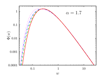
Figure 4: Wealth distribution according to Eq. (15) for $\epsilon\to 0$ (full line), $\epsilon=0.03$ (dashed line), $\epsilon=0.1$ (dash-dotted line), and $\epsilon=0.3$ (dotted line).

Let us stress again that the solution known for $\epsilon<0$ cannot be properly continued to the region of $\epsilon>0$, due to the presence of singularity at $\epsilon=0$. The singularity can be seeen e. g. in the behavior of the solution of Eq. (9), as shown in Fig. 5. However, for $\alpha=3/2$ the formula (13) describes the solution of (7) on both limits $\epsilon\to 0^{+}$ and $\epsilon\to 0^{-}$. This implies that the singularity is rather weak, because the solution of Eq. (7) is continuous in $\epsilon$, and only the derivative with respect of $\epsilon$ has a jump at $\epsilon=0$. One may speculate about the fate of the singularity if we allowed $\epsilon$ and $\beta$ not fixed parameters but random processes themselves. Most probably the singularity would vanish but final answer is left for future work.

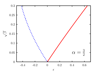
Figure 5: Solution of equation (9) for $\alpha=3/2$ in the ranges $\epsilon>0$ (full line) and $\epsilon<0$ (dashed line). Note the singularity at $\epsilon=0$ which means that we must skip from one of the three solutions of (9) to another one.

IV Conclusions

We formulated a model of wealth production and exchange, where agents randomly interact pairwise. Using the analogy with the mean-field version of the Maxwell model for inelastic scattering of granular particles we obtain analytical results for the wealth distribution.

The dynamics of the model is governed by a kinetic equation for one-particle distribution function. We look for self-similar scaling solutions, corresponding to redefining the unit of wealth after each wealth increase. The form of these solutions is given by a non-local differential equation, exactly soluble only in the practically irrelevant case of net wealth decrease. Therefore we turned to approximation schemes.

First, we looked at the behavior for large wealth. The tail of the wealth distribution has a power-law form, and its exponent $\alpha$ is determined by the interplay between the intensity of the wealth exchange and the amount of wealth produced. The form line in the $\beta$-$\epsilon$ plane with fixed $\alpha$ is found, depending quadratically on $\epsilon$ for $\epsilon\to 0$. The physically allowed values $\alpha\in(1,2)$ determine a horn-shaped region in the $\beta$-$\epsilon$ plane.

The second approximation consisted in taking the limit of continuous trading, meaning small wealth production and small exchange within a single trading operation, while keeping the exponent $\alpha$ constant. Here we obtained closed formula for the entire wealth distribution, which has power-law tail as expected and a maximum at certain (low) wealth value. The form of the wealth distribution corresponds to those found in previous studies sol_ric_01b ; ma_mas_zha_98 ; bou_mez_00 . It is interesting to note that this general form has one-to-one correspondence between the position $w_{\mathrm{max}}$ of the maximum of the distribution and the value of the exponent. There are few agents having wealth below $w_{\mathrm{max}}$. This suggests that the intuition formalized e. g. in sol_ric_01b ; solomon_99 , that the exponent is “tuned” by the low-wealth behavior of the distribution, may be in work quite generally. Here, the free parameters are apparently the wealth production and exchange, but in reality these parameters may be themselves tuned by a mechanism which fixes the position of the maximum of the wealth distribution, i. e. the lowest wealth compatible with survival.

However, there is still open question of the specific values of the exponent, which are quite robust in different societies. It seems, also on the basis of our results, that it cannot be explained by the bare mechanism of economic exchange and some other ingredient, possibly of sociological origin, is required.

Appendix A Systematic expansion for small $\epsilon$ and $\beta$.

Let us start with the special value $\alpha=3/2$. Here, the equation (9) has an explicit solution in the form

$$\epsilon=\frac{1}{8}\;{\frac{-3\,\sqrt{\beta}+17\,\beta-29\,{\beta}^{3/2}+15\,{\beta}^{2}+4\,{\beta}^{5/2}-4\,{\beta}^{3}+\sqrt{3}\sqrt{\left(3-2\,\sqrt{\beta}\right)\beta\,\left(2\,\sqrt{\beta}+1\right)^{3}\left(\sqrt{\beta}-1\right)^{6}}}{\sqrt{\beta}-3\,\beta+3\,{\beta}^{3/2}-{\beta}^{2}}}\;.$$ (16)

However, the non-local differential equation (7) still does not yield explicit solution. Inverting the expression (16) we get the following series expansion

$$\beta={\frac{1}{4}}{\epsilon}^{2}-{\frac{1}{12}}{\epsilon}^{3}+{\frac{1}{16}}{\epsilon}^{4}-{\frac{7}{144}}{\epsilon}^{5}+{\frac{113}{2592}}{\epsilon}^{6}+O\left({\epsilon}^{7}\right)\,.$$ (17)

For general value of $\alpha$ the variable $\beta$ is expressed as a series in two small parameters $\epsilon$ and $\eta=\epsilon^{2(\alpha-1)}$, which coincide only if $\alpha=3/2$. Therefore, we can write

$$\beta=\epsilon^{2}\,\sum_{m,n=0}^{\infty}\beta_{mn}\epsilon^{m+2(\alpha-1)n}$$ (18)

and the various terms take variable precedence in the order of smallness when $\epsilon\to 0$, depending on the value of $\alpha$. For the first several coefficients we have

$$\beta_{00} = \frac{\alpha-1}{2}$$ (19)

$$\beta_{10} = -\frac{(\alpha-1)(2\alpha-1)}{6}$$ (20)

$$\beta_{01} = \frac{1}{\alpha}\left(\frac{\alpha-1}{2}\right)^{\alpha}\;.$$ (21)

Starting from the expansion (18) we can convert the first order non-local differential equation (7) for $\hat{\Phi}(x)$ into infinite-order local differential equation for $\Phi(w)$. The price to pay for it is that the coefficients in the latter equation contain the moments $\mu_{k}=\int\Phi(w)w^{k}\mathrm{d}w$ of the solution itself. Indeed, we can write

$$\hat{\Phi}((1-\beta+\epsilon)\,x)=\lim_{y\to x}\exp\left((\epsilon-\beta)\,x\frac{\mathrm{d}}{\mathrm{d}y}\right)\,\hat{\Phi}(y)$$ (22)

$$\hat{\Phi}(\beta x)=\lim_{y\to 0}\exp\left(\beta\,x\frac{\mathrm{d}}{\mathrm{d}y}\right)\,\hat{\Phi}(y)\;.$$ (23)

Therefore, we obtain a linear combination of terms of the following form

$$x^{m+n}\,\frac{\mathrm{d}^{m}\hat{\Phi}(x)}{\mathrm{d}x^{m}}\,\frac{\mathrm{d}^{n}\hat{\Phi}(0)}{\mathrm{d}x^{n}}$$ (24)

which, after inverse Laplace transform, give rise to terms

$$(-1)^{m+n}\,\mu_{n}\,\frac{\mathrm{d}^{m+n}}{\mathrm{d}w^{m+n}}\,\left[w^{m}\,\Phi(w)\right]\;.$$ (25)

However, the first two moments are fixed by definition. Indeed, the normalization of the probability distribution fixes the zeroth moment and the fixed average wealth, imposed by the scaling condition (6) fixes the first moment, so that $\mu_{0}=\mu_{1}=1$. This consideration leads to the equations for lowest correction to the solution (13), which are free of unknown higher moments.

Generally, the solution can be then expressed in the form of the series in powers of $\epsilon$ and $\epsilon^{2(\alpha-1)}$

$$\Phi(w)=\Phi_{0}(w)\sum_{m,n=0}^{\infty}\phi_{mn}(w)\,\epsilon^{m+2(\alpha-1)n}\;.$$ (26)

We assume $\phi_{00}(w)=1$. The normalization must be independent of $\epsilon$, which can be written as

$$\int_{0}^{\infty}\Phi_{0}(w)\phi_{mn}(w)\mathrm{d}w=\delta_{m0}\delta_{n0}\;.$$ (27)

Therefore, the lowest term obeys the equation

$$\frac{w^{2}}{2}\Phi_{0}^{\prime}(w)+\left(\frac{\alpha+1}{2}w-\frac{\alpha-1}{2}\right)\Phi_{0}(w)=0$$ (28)

which has the following solution satisfying the normalization (27)

$$\Phi_{0}(w)=\frac{(\alpha-1)^{\alpha}}{\Gamma(\alpha)}\,w^{-1-\alpha}\exp\left(\frac{1-\alpha}{w}\right)\;.$$ (29)

Indeed, it coincides with the result of (13).

The next two terms satisfy the following equations

$$\frac{w^{2}}{2}\phi_{10}^{\prime}(w)=\frac{\alpha-1}{3}\,\left(\alpha-\frac{\alpha-1}{w}\right)$$ (30)

$$\frac{w^{2}}{2}\phi_{01}^{\prime}(w)=-\frac{1}{\alpha}\,\left(\frac{\alpha-1}{2}\right)^{\alpha}\,\left(w-1\right)$$ (31)

which can be easily solved. We obtain

$$\phi_{10}(w) = -\frac{\alpha-1}{3}\,\left(\frac{2\,\alpha}{w}-\frac{\alpha-1}{w^{2}}-\nu_{10}\right)$$ (32)

$$\phi_{01}(w) = -\frac{2}{\alpha}\left(\frac{\alpha-1}{2}\right)^{\alpha}\left(\ln w+\frac{1}{w}-\nu_{01}\right)$$ (33)

and the constants $\nu_{01},\nu_{10}$ are fixed by the normalization condition (27). We find explicitly

$$\nu_{10} = \alpha$$ (34)

$$\nu_{01} = \ln\left(\alpha-1\right)-\Psi\left(\alpha\right)+\frac{\alpha}{{\alpha}-1}$$ (35)

where $\Psi(x)=\Gamma^{\prime}(x)/\Gamma(x)$ is the logarithmic derivative of the gamma function.

References

- (1) V. Pareto, Cours d’economie politique, (Lausanne, F. Rouge, 1897).
- (2) M. Levy and S. Solomon, Physica A 242, 90 (1997).
- (3) A. Drăgulescu and V. M. Yakovenko, Physica A 299, 213 (2001).
- (4) W. J. Reed and B. D. Hughes, Phys. Rev. E 66, 067103 (2002).
- (5) H. Aoyama, W. Souma, and Y. Fujiwara, Physica A 324, 352 (2003).
- (6) A. Y. Abul-Magd, Phys. Rev. E 66, 057104 (2002).
- (7) M. Levy and S. Solomon, Int. J. Mod. Phys. C 7, 595 (1996).
- (8) M. Levy and S. Solomon, Int. J. Mod. Phys. C 7, 65 (1996).
- (9) O. Biham, O. Malcai, M. Levy, and S. Solomon, Phys. Rev. E 58, 1352 (1998).
- (10) S. Solomon, in: Decision technologies for Computational Finance, ed. A.-P. Refenes, A. N. Burgess, and J. E. Moody (Kluwer Academic Publishers, 1998).
- (11) S. Solomon, in: Application of Simulation to Social Sciences, ed. G. Ballot and G. Weisbuch (Hermes Science Publications, 2000).
- (12) Z.-F. Huang and S. Solomon, Eur. Phys. J. B 20, 601 (2001).
- (13) S. Solomon and P. Richmond, Physica A 299, 188 (2001).
- (14) A. Blank and S. Solomon, Physica A 287, 279 (2000).
- (15) S. Solomon and M. Levy, cond-mat/0005416.
- (16) Z.-F. Huang and S. Solomon, Physica A 294, 503 (2001).
- (17) D. Sornette and R. Cont, J. Phys I France 7, 431 (1997).
- (18) D. Sornette, Physica A 250, 295 (1998).
- (19) D. Sornette, Phys. Rev. E 57, 4811 (1998).
- (20) H. Takayasu, A.-H. Sato, and M. Takayasu, Phys. Rev. Lett. 79, 966 (1997).
- (21) M. Marsili, S. Maslov, and Y.-C. Zhang, Physica A 253, 403 (1998).
- (22) J.-P. Bouchaud and M. Mézard, Physica A 282, 536 (2000).
- (23) Z. Burda, D. Johnston, J. Jurkiewicz, M. Kamiński, M. A. Nowak, G. Papp, and I. Zahed, cond-mat/0101068.
- (24) W. Souma, cond-mat/0011373.
- (25) H. Aoyama, Y. Nagahara, M. P. Okazaki, W. Souma, H. Takayasu, M. Takayasu, cond-mat/0006038.
- (26) W. Souma, cond-mat/0202388.
- (27) W. Souma, Y. Fujiwara, and H. Aoyama, cond-mat/0108482.
- (28) Y. Fujiwara, W. Souma, H. Aoyama, T. Kaizoji, and M. Aoki, cond-mat/0208398.
- (29) A. Chakraborti and B. K. Chakrabarti, Eur. Phys. J. B 17, 167 (2000).
- (30) B. K. Chakrabarti and A. Chatterjee, in: Applications of Econophysics, Conference proceedings of Second Nikkei Symposium on Econophysics, Tokyo, Japan, 2002 (Springer-Verlag, Tokyo, 2003) pp. 280-285; cond-mat/0302147.
- (31) A. Chatterjee, B. K. Chakrabarti, and S. S. Manna, cond-mat/0301289, to be published in Physica A; Phys. Scripta T106, 36 (2003); cond-mat/0311227.
- (32) A. Das and S. Yarlagadda, cond-mat/0304685.
- (33) S. Pianegonda, J. R. Iglesias, G. Abramson, and J. L. Vega, Physica A 322, 667 (2003).
- (34) J. R. Iglesias, S. Gonçalves, S. Pianegonda, J. L. Vega, and G. Abramson, Physica A 327, 12 (2003).
- (35) S. Pianegonda and J. R. Iglesias, cond-mat/0311113.
- (36) J. R. Iglesias, S. Gonçalves, G. Abramson, and J. L. Vega, cond-mat/0311127.
- (37) M. Anazawa, A. Ishikawa, T. Suzuki, and M. Tomoyose, cond-mat/0307116.
- (38) T. Mizuno, M. Katori, H. Takayasu, and M. Takayasu, cond-mat/0308365.
- (39) T. Mizuno, M. Takayasu, and H. Takayasu, cond-mat/0307270.
- (40) Y. Fujiwara, C. Di Guilmi, H. Aoyama, M. Gallegati, and W. Souma, cond-mat/0310061.
- (41) A. Drăgulescu and V. M. Yakovenko, Eur. Phys. J. B 17, 723 (2000); Eur. Phys. J. B 20, 585 (2001); in: Modeling of Complex Systems: Seventh Granada Lectures, AIP Conference Proceedings 661 , 180 (New York, 2003).
- (42) V. M. Yakovenko, cond-mat/0302270.
- (43) S. Ispolatov, P. L. Krapivsky, and S. Redner, Eur. Phys. J. B 2, 267 (1998).
- (44) N. Scafetta, S. Picozzi, and B. J. West, cond-mat/0209373.
- (45) N. Scafetta and B. J. West, cond-mat/0306579.
- (46) M. Gligor and M. Ignat, Eur. Phys. J. B 30, 125 (2002).
- (47) S. Sinha, cond-mat/03043224.
- (48) H. M. Jaeger, S. R. Nagel, and R. P. Behringer, Rev. Mod. Phys. 68, 1259 (1996).
- (49) A. V. Bobylev, J. A. Carillo, and I. M. Gamba, J. Stat. Phys. 98, 743 (2000).
- (50) A. V. Bobylev and C. Cercignani, J. Stat. Phys. 106, 547 (2002); J. Stat. Phys. 110, 333 (2003).
- (51) A. Baldassarri, U. Marini Bettolo Marconi, and A. Puglisi, Europhys. Lett. 58, 14 (2002).
- (52) I. Ispolatov and P. L. Krapivsky, Phys. Rev. E 61, R2163 (2000).
- (53) E. Ben-Naim and P. L. Krapivsky, Phys. Rev. E 61, R5 (2000).
- (54) P. L. Krapivsky and E. Ben-Naim, J. Phys. A: Math. Gen. 35, L147 (2002).
- (55) E. Ben-Naim and P. L. Krapivsky, Phys. Rev. E 66, 011309 (2002).
- (56) D. ben-Avraham, E. Ben-Naim, K. Lindenberg, and A. Rosas, Phys. Rev. E 68, 050103 (2003).
- (57) M. H. Ernst and R. Brito, Europhys. Lett. 58, 182 (2002).
- (58) M. H. Ernst and R. Brito, cond-mat/0111093; Phys. Rev. E 65, 040301 (2002); J. Stat. Phys. 109, 407 (2002); Europhys. Lett. 58, 182 (2002); cond-mat/0304608.
- (59) E. Ben-Naim and P. L. Krapivsky, cond-mat/0301238.
- (60) T. Antal, M. Droz, and A. Lipowski, Phys. Rev. E 66, 062301 (2002).
- (61) E. Barkai, Phys. Rev. E 68, 055104 (2003).
- (62) A. Baldassarri, U. Marini Bettolo Marconi, and A. Puglisi, cond-mat/0105299.
- (63) A. Baldassarri, U. Marini Bettolo Marconi, A. Puglisi, and A. Vulpiani, Phys. Rev. E 64, 011301 (2001).
- (64) D. J. Watts and S. H. Strogatz, Nature 393, 440 (1998).
- (65) A.-L. Barabási and R. Albert, Science 286, 509 (1999).
- (66) T. Di Matteo, T. Aste, and S. T. Hyde, cond-mat/0310544.