Renormalization group and Ward identities in quantum liquid phases and in unconventional critical phenomena

Abstract

By reviewing the application of the renormalization group to different theoretical problems, we emphasize the role played by the general symmetry properties in identifying the relevant running variables describing the behavior of a given physical system. In particular, we show how the constraints due to the Ward identities, which implement the conservation laws associated with the various symmetries, help to minimize the number of independent running variables. This use of the Ward identities is examined both in the case of a stable phase and of a critical phenomenon. In the first case we consider the problems of interacting fermions and bosons. In one dimension general and specific Ward identities are sufficient to show the non-Fermi-liquid character of the interacting fermion system, and also allow to describe the crossover to a Fermi liquid above one dimension. This crossover is examined both in the absence and presence of singular interaction. On the other hand, in the case of interacting bosons in the superfluid phase, the implementation of the Ward identities provides the asymptotically exact description of the acoustic low-energy excitation spectrum, and clarifies the subtle mechanism of how this is realized below and above three dimensions. As a critical phenomenon, we discuss the disorder-driven metal-insulator transition in a disordered interacting Fermi system. In this case, through the use of Ward identities, one is able to associate all the disorder effects to renormalizations of the Landau parameters. As a consequence, the occurrence of a metal-insulator transition is described as a critical breakdown of a Fermi liquid.

Keywords: Renormalization group; Ward identities; many-body theory.

1 Introduction

There exist several physical problems where the use of simple perturbative methods seems to be deemed to failure from the start. In these cases, already in the leading perturbative correction, one faces singular terms which render the perturbative expansion meaningless, no matter how small the initial expansion parameter is. The great success of the renormalization group (RG) has been to turn, at least in a number of highly non-trivial cases, this apparent failure into a powerful tool. The RG conceptual scheme [1, 2] teaches us how singular terms, arising in the perturbative expansion, give rise to the power-law and scaling behaviors characteristic of the critical phenomena [3, 4, 5, 6]. This is the most successful use of the RG, which we only briefly recall in Sec. 2. In particular, we introduce the basic elements of the RG approach such as universality, scaling, relevant and irrelevant variables, and discuss the Wilson[2] and the field-theoretic RG[7, 5, 8], which can be seen as two different implementations of universality.

The origin of a singular perturbation theory is understood within the $\varphi^{4}$ model for critical phenomena, where $\varphi({\bf r})$ is the field whose thermal average specifies the order parameter $\varphi_{0}$ [9]. Indeed, the dimensionless effective coupling constant which appears in perturbation theory in $d$ spatial dimensions is $u/|t|^{\epsilon/2}$, where $\epsilon=4-d$, $u$ is the coupling constant describing the self-interaction of the fluctuations of the field $\varphi$, and $t=T-T_{c}$ measures the deviation of the temperature $T$ from the critical temperature $T_{c}$. This leads to a divergence when approaching criticality ($t\to 0$), for $\epsilon>0$ ($d<4$) [for the corresponding power counting, leading to the expression of the dimensionless coupling constant given above, see Fig. 1(a)]. The RG sums the leading singularities into power laws for the order parameter $\varphi_{0}\sim|t|^{\beta}$, for the susceptibility $\chi\sim|t|^{-\gamma}$, which measures the linear response to its conjugate external field $h$, for the specific heat $C\sim|t|^{-\alpha}$, etc. Here, $\beta,\gamma,\alpha$… are called the critical exponents, or critical indices.

We will also turn our attention to different uses of the RG approach. One class of such applications is met when the critical behavior is unconventional. This may occur, for instance, when it is difficult to identify the order parameter (which can be a complicated object, or a composite operator) and the related broken symmetry. The problem of the metal-insulator transition (MIT) in a disordered interacting electron system is an important example of this class [10, 11, 12, 13, 14, 15, 16]. In this case the symmetries of the physical problem may provide the guiding framework to identify the effective theory. These symmetries can be translated into Ward identities which establish relations among the various terms of the skeleton structure of the problem, simplifying the RG treatment.

The use of the RG, however, is not limited to the critical behavior. It turns out to be extremely useful also in the stable phases. Indeed, there are cases in which a divergent perturbation theory is the result of relevant low-lying excitations in low-dimensional systems, despite the fact that the system is in a stable liquid phase of the matter. This is the case, e.g., of the Luttinger liquid in one-dimensional interacting Fermi systems [17] [see Fig. 1(b)], or of Bose liquids in the superfluid phase for $d\leq 3$ [18, 19] [see Fig. 1(c),(d)]. The very condition of phase stability implies that the susceptibilities (e.g., specific heat, spin susceptibility, compressibility, etc.) are finite, and the exact cancellation of the singular contributions is controlled by Ward identities. Nonetheless, as we shall show, a track of the singularities is usually left in the power-law behavior of some one-particle physical quantities.

In the following, we will touch upon all these examples, often stressing the key role played in practice by the Ward identities which implement the fundamental symmetries of the physical system at hand, and for the last two cases allow for a complete solution of the low-lying excitation problem. The rest of the paper is organized as follows. In Sec. 2, we recall a few basic concepts about the RG and how Ward identities may be used to carry out the renormalization program. In Sec. 3, we discuss the application of RG to stable phases. First, in Sec. 3.1, we examine the case of interacting fermions in one [20, 21] and low dimensions [22, 23, 24, 25]. Then, in Sec. 3.2, we analyze the problem of interacting bosons [26, 27]. In Sec. 4, we focus our attention on the problem of disordered interacting Fermi systems [28, 29, 30, 31, 32, 33, 34, 35, 36, 37, 38, 39].

2 The renormalization group and the Ward identities

2.1 General remarks on the group transformation

The first aspect that must be appreciated by looking at the historical development of the RG is the change of perspective with respect to the reduction scheme which, before its introduction, was at work in formulating a condensed-matter theory. The fifties and the sixties of the past century had seen the flourishing of the quasiparticle concept. According to this, an interacting system may be effectively described in terms of “almost” independent elementary excitations (quasiparticles). Implicit in this attitude is the privileged role reserved to the “approximate” solution of the dynamical problem and to the development of the many-body theory, with respect to the statistical aspects. In the late sixties and early seventies, the realization of the importance of the large-scale fluctuations in approaching the critical point shifted the attention onto the statistical problem [40, 41]. The divergence of the correlation length $\xi\sim|t|^{-\nu}$, when $t\to 0$, implies the strong correlation of a large number of degrees of freedom within a region of an increasing linear size $\xi$, and then invalidates the previous quasiparticle-based reduction schemes. The collective critical phenomenon does not arise as a simple superposition of single microscopic events. Through the action of ordering forces, the probability distribution of the collective variables no longer obeys the central limit theorem, according to which the correct normalization for an extensive variable is provided by the square root of the number of degrees of freedom. This violation, via an anomalous normalization of block variables, is the mathematical manifestation of the existence of correlations at all length scales, so that the crucial hypothesis of statistical independence becomes progressively not applicable getting closer to the critical point.

The very fact that $\xi\to\infty$ when approaching criticality, while invalidating the previous reduction schemes, provides the crucial key for the new reduction scheme, i.e., universality [40, 41].

There are two equivalent forms of universality. First of all, the microscopic details which specify the peculiarities of each individual system become gradually irrelevant when approaching criticality, and the infinitely large number of degrees of freedom involved is well accounted for by a small set of relevant variables. Once the proper choice of the relevant variables is made (e.g., $t$ and $h$ or $\varphi$), one can change the parameters $\zeta_{i}$ which specify the microscopic details (unless they assume a value which changes the symmetry of the problem, thus becoming relevant), without changing the critical behavior of the system. Said in other words, systems which differ in the irrelevant variables share the same critical behavior [42]. This condition translates into the invariance of the (singular part of the) free energy ${\cal F}$, or equivalently of its Legendre transform $\Gamma=\int d^{d}{\bf r}~{}h\varphi-{\cal F}$,

$${\cal F}(t,h;\{\zeta_{i}\}) = {\cal F}(t^{\prime},h^{\prime};\{\zeta_{i}^{\prime}\}),$$

$$\Gamma(t,\varphi;\{\zeta_{i}\}) = \Gamma(t^{\prime},\varphi^{\prime};\{\zeta_{i}^{\prime}\}),$$

i.e., a suitable rescaling of the relevant variables fully accounts for a change in the irrelevant variables.

The second form of universality relies on the fact that the unit length scale is irrelevant when $\xi\to\infty$. This is translated into the statement that one can eliminate the degrees of freedom at short distance, by grouping microscopic variables into “block variables”, within an iterated procedure to build larger and larger blocks, without changing the critical behavior of the system [41].

The field-theoretic RG equations generalize the universality relations in the sense that they relate one model system to another by varying the coupling constant $\zeta$ and suitably rescaling the other variables and the correlation functions [7]. In ordinary critical phenomena, described by the $\varphi^{4}$ theory, $\varphi$ (wave-function) and $t$ (mass) must be rescaled. When the coupling reaches its fixed point, a two-parameter scaling follows.

The Wilson new RG implements the second idea of universality illustrated above, by eliminating the short-wavelength fluctuations of the field $\varphi$, i.e., those with characteristic momenta $\Lambda/s<q<\Lambda$, where $\Lambda$ is the ultraviolet cutoff, and $s$ is the scaling parameter [2]. The real space version of the Wilson RG implementation is the bloc variable transformation[43, 44, 45, 46].

The calculation of the critical indices was performed either numerically, through recurrence equations, or analytically, within the $\epsilon$ expansion [47]. This latter procedure relies on the perturbative expansion of the RG transformation in the parameter $\epsilon=4-d$, starting from the known case $d=4$. The direct calculation of the divergent critical quantities is thus avoided.

In general, a sets of parameters $\{\mu_{j}\}$ specifies a given Hamiltonian $H$ in the space ${\cal H}$ of the Hamiltonians. The action of the RG transformation ${\cal R}_{s}$ (which depends on the scaling parameter $s$) in this space preserves the functional $\Gamma$, so that symbolically [44, 45]:

$$\Gamma[{\cal R}_{s}[H]]=\Gamma[H].$$

The above equation can be written in a differential form as

$$d_{{\cal R}_{s}}\Gamma=0.$$

The functional derivatives of $\Gamma$ yield the group equations for all the physical quantities.

A fixed point of the transformation is such that $H^{*}={\cal R}_{s}[H^{*}]$. At criticality $\xi=\infty$ and it remains infinite under iteration of RG transformations. By iteration of the group transformation on the critical surface one model Hamiltonian is transformed into another, until a fixed-point simplified Hamiltonian is reached as $s\to\infty$, which is manifestly scale invariant, and all the irrelevant transient terms have been eliminated. The relevant parameters define a finite set of relevant directions of escape from a given fixed point [48], and their scale dependence gives a microscopic definition of the critical indices. Universality corresponds to the domain of attraction of a given fixed point. Within a given domain, the transformations become asymptotically equivalent[43, 44].

Standard renormalizability implies that the removal of the ultraviolet cutoff, $\Lambda\sim 1/a\to\infty$ (where $a$ is the lattice spacing or some other microscopic characteristic length scale) only requires the definition of a finite (small) set of renormalized parameters. Relevant parameters and renormalized parameters coincide asymptotically in the infrared region.

Here a general problem arises. Recently, a renewed attention has been devoted to the exact RG equations [49]. In practice, however, one has to truncate these equations or reduce the number of flow parameters. In this last case, one has to initialize the action to follow a renormalized trajectory with a small number of flowing parameters, and an infinite set of parameters in the action must be specified. This specification is a highly non-perturbative condition.

In practice, therefore, one should rather choose the best simple action, guided by the symmetries of the problem and by the physical conditions. The knowledge of the fundamental symmetries inherent to each specific problem, and in particular those of the order parameter, have to be assumed in order to make the proper choice of the basic variables on which the RG transformation acts.

2.2 Various exploitations of the Ward identities

The RG approach takes enormous advantage from the explicit implementation of the symmetries of the original problem, which translate into Ward identities relating various independent quantities.

First of all, the Ward identities allow for a reduction of the renormalization parameters. The case of quantum electrodynamics is a textbook example. The local $U(1)$ gauge invariance of the Lagrangian, which is invariant under the simultaneous transformation of the phonon field $A_{\nu}\to A_{\nu}+\partial_{\nu}\vartheta$ and of the fermion field $\psi\to\psi{\rm e}^{ie\vartheta}\simeq(1+ie\vartheta)\psi$, where $\vartheta$ is the gauge field, allows to relate the self-energy and vertex renormalizations, whose corrections correspond to superficially divergent diagrams within perturbation theory in $d=3+1$ dimensions.

Secondly, the Ward identities provide the guiding framework for the identification of the proper running variables (effective coupling constants), and how they are related to physical quantities. We will consider the case of disordered interacting electron systems. As we shall see, the various interaction amplitudes are dressed by disorder. The renormalization parameters of the corresponding field-theoretical formulation of the problem (the non-linear $\sigma$-model [28, 14]) are identified in terms of physical quantities of the Fermi-liquid theory by requiring the gauge invariance of the skeleton structure of the response functions [10, 31, 32, 36, 37].

Finally, the Ward identities control the exact cancellation of the singularities in the various response functions within stable phases, despite a singular perturbation theory. In these cases, indeed, specific symmetries are related to additional Ward identities, which enforce the cancellations.

The combination of the three procedures indicated above leads to the asymptotically exact description of: the Luttinger liquid in $d=1$ [17, 20], and its crossover to the Fermi liquid in $d>1$ [22, 23]; the non-Fermi-liquid behavior of an interacting electron system with singular forward scattering in $d>1$ [24, 25]; the Bose liquid in the presence of the Bose-Einstein condensate [26]; the disordered interacting electron systems [28, 31]. In Tab. 1 we provide a scheme of the symmetries and Ward identities which are relevant in the various physical problems discussed in this paper.

Each specific system has been discussed at length in several papers. We emphasize here the general common aspects and give a unifying view of these apparently very different theoretical problems.

3 Renormalization group and stable phases

As we have already indicated in Sec. 1, there are cases where the perturbation theory is singular even in a stable phase. We first recall here the case of the Luttinger liquid in one dimension, its dimensional crossover to a Fermi liquid as soon as $d>1$ in the presence of short range forces, and the non-Fermi-liquid behavior when the forces among the fermions are sufficiently singular. We then consider the low-lying excitations from a ground state of bosons in the presence of interaction, where the condensate changes the power counting and leads to singular terms in perturbation theory for $1<d\leq 3$. The use of the RG, in these cases, acquires a different meaning with respect to critical phenomena, as the thermodynamic stability implies here a cancellation of singularities at any order in perturbation theory in all the susceptibilities, like specific heat, compressibility, etc. Behind these exact cancellations there must be specific symmetry properties, which can be used in the form of Ward identities to close the hierarchy of RG equations and solve the problem. Although a stable system is characterized by finite response functions, the re-summation of singularities may still manifest itself with an anomalous dimension as in the one-particle fermion Green’s function.

3.1 Interacting fermions in low dimensions

Within a RG approach, the effective low-energy Hamiltonian which describes a metallic system can be obtained via the Wilson-like iterative elimination of states outside a shell of thickness $\Lambda$ around the Fermi surface [17, 23, 50]. As $\Lambda$ is iteratively scaled to zero a fixed point is reached in $d=3$ which corresponds to a gas of quasiparticles with finite residual Hartree-like interaction, described by the Landau functional. Ordinary three-dimensional metals are thus well described by the Landau Fermi-liquid theory [51]. The interaction is effectively taken into account in the various response function through a small set of Landau parameters, entering the physical quantities, e.g., the specific-heat coefficient $\gamma=C_{V}/T$, the spin susceptibility $\chi$, the compressibility $\partial n/\partial\mu$, and the spectral weight of the Drude peak in the optical conductivity, all of them being finite.

A finite wave-function renormalization $Z<1$ reduces the discontinuity of the occupation number in momentum space at the Fermi surface with respect to the value of the Fermi gas ($Z=1$). The elementary excitations of the system are the single-particle excitations (quasiparticles), which carry both charge and spin, and the collective charge and spin modes, which get overdamped when they enter the particle-hole continuum of excitations.

In recent times, the interest for non-Fermi-liquid metallic phases has been rekindled by the observation of anomalous features in single-particle and transport properties of the cuprates, which have been interpreted as a signature of non-Fermi-liquid behavior [52]. These compounds are layered (quasi-two-dimensional) materials, which are insulating when stoichiometric, and become metallic upon chemical doping. The metallic phase is strongly anomalous at low doping and gradually (and smoothly) evolves towards a Fermi-liquid-like metal at large doping.

The breakdown of the Fermi liquid could be produced by the suppression of quasiparticle spectral weight at the Fermi surface due to the generation of an interaction-induced anomalous dimension in the wave-function renormalization, $Z\sim|p-p_{F}|^{\eta}$, where $p-p_{F}$ measures the deviation of the quasiparticle momentum $p$ from the Fermi momentum $p_{F}$. In such a case, $Z$ vanishes as $p\to p_{F}$, the low-lying single-particle excitations are completely suppressed, and the low-energy behavior of the system is dominated by the charge and spin collective modes. Since these have, in general, different velocities, the system is characterized by the so-called charge and spin separation.

This behavior is achieved in $d=1$, where the metallic phase is a Luttinger liquid. The hint for the breakdown of the Fermi-liquid picture is given by the appearance of logarithmic singularities in perturbation theory as $p\to p_{F}$ [see Fig. 1(b)]. These singularities are controlled by the RG, and an effective field theory results, with marginal forward scattering, the so-called Luttinger model, which is exactly solvable. Additional conservation laws, which are peculiar to one-dimensional systems with forward scattering, constrain the model and lead to a closure of the equations of motion.

Indeed, the total charge and spin conservation is translated into the usual Ward identity

$$\omega\Lambda_{0}-{\bf q}\cdot{\mathbf{\Lambda}}=G^{-1}(\varepsilon+\omega,{\bf p}+{\bf q})-G^{-1}(\varepsilon,{\bf q}),$$ (1)

which connects the irreducible density ($\Lambda_{0}$) and current (${\mathbf{\Lambda}}$) vertices to the electronic Green’s function $G$. In addition, in this case, charge and spin are separately conserved at each Fermi point $p=\pm p_{F}$, leading to an additional Ward identity [20] stating the proportionality of the current vertex to the density vertex, due to the unique momentum direction,

$${\mathbf{\Lambda}}=v_{F}{\hat{\bf p}}\Lambda_{0},$$ (2)

where $v_{F}$ is the Fermi velocity and the direction versor ${\hat{\bf p}}$ here ($d=1)$ is $\pm 1$. By means of the two Ward identities (1) and (2) one is able to express the density vertex $\Lambda_{0}$ as a function of the fermion propagator $G$, thus closing the Dyson equation of Fig. 2.

The effective interaction $D$ (which is represented by the tick-dashed line in Fig. 2) contains the charge and spin collective modes via the RPA re-summation of the bare interaction with the fermion polarization bubble. The RPA re-summation is shown to be exact by the use of the same Ward identities (1) and (2). As a result density and spin response functions are finite, leading to a stable metallic phase.

On the contrary, from the exact evaluation of $G$ one finds that its behavior is controlled by a non-universal anomalous dimension $\eta$. Single particles hence move as composite objects due to the strong mixing with the charge and spin collective modes, induced by the effective interaction.

The question then arises whether the Luttinger-liquid behavior can be extended to higher dimensions. The analysis of the dimensional crossover shows that this is not possible if the interactions are short-ranged. Indeed, the generic integrals in $d$ dimensions

$$\int d^{d}{\bf q}~{}f({\bf q},{\bf p}\cdot{\bf q})=S_{d-1}\int dq~{}q^{d-1}\int_{0}^{\pi}d\theta(\sin\theta)^{d-2}f(q,pq\cos\theta),$$

where $S_{d-1}$ is the solid angle in $d-1$ dimensions, are strongly peaked at $\theta=0,\pi$ for $1\leq d<2$, so that all the relevant vectors are still parallel or antiparallel. In this case, the additional Ward identity (2) is still valid asymptotically near the Fermi surface. However, the mixing with the collective modes is reduced as soon as $d>1$, since the effective interaction $D({\bf q},\omega)$ is averaged over the $d-1$ momentum components perpendicular to the Fermi momentum. The effective interaction, which is marginal in $d=1$, scales to zero for $d>1$, and the system is a Fermi liquid.

However, if we consider a long-range bare interaction among the fermions, $V(q)\sim q^{-\alpha}$, the effective interaction dressed by the RPA series is

$$D({\bf q},\omega)=\frac{1}{q^{\alpha}}~{}\frac{\omega^{2}}{\omega^{2}-c^{2}q^{2-\alpha}},$$ (3)

and is dominated by a collective mode $\omega(q)=cq^{1-\alpha/2}$, which is propagating and gapless for $\alpha<2$ (the parameter $c$ depends on the microscopic parameters of the fermion model, and does not acquire singular corrections, see below). This singular behavior as $q\rightarrow 0$ compensates the rescaling to zero of the effective interaction due to its averaging over the transverse momentum and leads to a non-Fermi-liquid behavior for $\alpha\geq 2d-2$ [24].

A singular interaction may appear in a system close to an instability, due to the coupling of the fermion quasiparticles with the critical fluctuations. Various proposals for the breakdown of the Fermi-liquid picture in the cuprates rely on the existence of a quantum critical point in their phase diagram [53].

The problem of fermions interacting via a singular interaction is plagued by infrared divergences and requires a proper RG treatment, supported by the Ward identities [25].

The vertex $\Lambda_{0}$ induces a coupling constant $g$ which in principle contains the divergences of the vertex (which requires the renormalization $Z_{V}$), of the fermion propagator (renormalized by $Z$) and of the collective-mode propagator $D$ (renormalized by $Z_{D}$). The coupling is accordingly renormalized as $g_{0}=gZZ_{D}^{1/2}/Z_{V}$. However, the total charge conservation translated into the usual Ward identity (1), gives, in the dynamic limit,

$$Z_{V}^{-1}=\lim_{\omega\to 0}\lim_{{\bf q}\to 0}\Lambda_{0}=\partial_{\varepsilon}G^{-1}\equiv Z^{-1}.$$ (4)

Moreover, since small-${\bf q}$ scattering dominates, the charge is asymptotically conserved at each point of the Fermi surface, leading to the additional Ward identity (2). When the vertex $\Lambda_{0}$ is accordingly expressed in terms of the fermion propagator $G$, one realizes that the effective interaction $D$, i.e., the collective-mode propagator (3) does not get anomalous corrections beyond the RPA approximation, i.e., $Z_{D}=1$. In fact, the vertex corrections to the bare polarization bubble asymptotically cancel with the selfenergy corrections, thank to the additional Ward identity (2).

Therefore, together with Eq. (4), this implies that $g=g_{0}$, and the dimensionless running coupling constant $u=g_{0}^{2}/s^{x_{u}}$, where $s$ is some infrared cutoff which plays the role of the scaling parameter, evolves under RG with its bare dimension $x_{u}=1-d+\alpha/2$ as $s\to 0$. Therefore at the dimension $d=d_{c}\equiv 1+\alpha/2$ the coupling is marginal ($x_{u}=0$). For $d<d_{c}$ the bare dimension $x_{u}$ is positive, the theory scales to strong coupling and the Fermi liquid breaks down. Finally, for $d>d_{c}$, $x_{u}$ is negative and the effective coupling scales to zero. Thus $Z$ stays finite and the system is a Fermi liquid.

From the one-loop perturbative RG, one finds the explicit form of the wave-function renormalization as a function, e.g., of the quasiparticle energy $\varepsilon$. At $d=d_{c}$, $Z\sim|\varepsilon|^{u_{0}}$, vanishes with a non-universal exponent $u_{0}\sim g_{0}^{2}$, as in the Luttinger liquid. For $d<d_{c}$, instead, $Z$ scales to zero as a stretched exponential, for $\varepsilon\to 0$. In both cases, the single-particle spectral weight is suppressed as the Fermi surface is approached.

3.2 Interacting bosons in low dimensions

The theory of the interacting Bose system has been motivated by the observation of superfluidity in liquid helium for $T<T_{\lambda}=2.17$K. The connection between the form of the spectrum of the low-lying excitations and the superfluid properties of the system was established by Landau via the criterion which requires a finite minimum slope of the quasiparticle dispersion $\varepsilon({\bf q})$ [54].

The simplest interacting Bose system assumes a quartic contact interaction $v$ for the boson field $\varphi$. The mean-field solution due to Bogoljubov [55], is obtained by linearizing the interaction term via the factorization of the condensate density $n_{0}^{1/2}=\langle\varphi\rangle=\langle\varphi^{\dagger}\rangle$. The free-particle spectrum $q^{2}/2m$ is converted at low momenta into a linear spectrum $\varepsilon({\bf q})=\sqrt{2n_{0}v}q\equiv c_{0}q$, characteristic of a sound-like excitation in the liquid, leading to superfluidity.

However, the Bogoljubov solution leads to a non-zero anomalous self-energy $\bar{\Sigma}=v\langle\varphi\varphi\rangle=vn_{0}$. Moreover, the first corrections to the Bogoljubov approximate solution, within the so-called pairing approximation, lead to a spurious gap in the excitation spectrum [56]. Both these results are in contrast with exact results, which show that no gap is present in the spectrum (Hugenoltz-Pines theorem) [57], and that the anomalous self-energy vanishes, $\bar{\Sigma}\equiv 0$ [58].

On the other hand, standard perturbation theory is plagued by infrared divergences in $d\leq 3$, due to the Goldstone sound mode [18, 19], despite the fact that the superfluid phase is a stable liquid phase of matter. All these aspects call for a cautious analysis of the problem, as it was first recognized in Ref. [19]. Benfatto used the Wilson RG approach to determine the scaling behavior for a number of running variables [27]. However, his treatment was limited to $d=3$ and did not take advantage of a systematic implementation of the Ward identities. We summarize the results in generic $d$ dimensions, fully exploiting the Ward identities, along the lines of Ref. [26].

Within the standard formulation of the problem, an external source $A_{\nu}=(\mu({\bf r}),{\bf A}({\bf r}))$, $\nu=0,...,d$, coupled to the boson density (current) and a field $h({\bf r})$ conjugate to $\varphi({\bf r})$ are introduced to generate the correlation functions. The original problem is recovered when ${\bf A}\to 0$, $h\to 0$ and $\mu$, taken as a constant, is identified with the chemical potential of the liquid. By introducing the longitudinal and transverse components to the direction along which the symmetry is broken, we have $\varphi=\varphi_{L}+{\rm i}\varphi_{T}$, with $\langle\varphi_{L}\rangle_{h\to 0}=\sqrt{n_{0}}$, and $h=h_{L}+{\rm i}h_{T}$. Functional derivatives of the free energy ${\cal F}[A_{\nu},h_{i}]$ with respect to the external sources produce the various density, current expectation values and Green’s functions, e.g., $\varphi_{i0}({\bf r})\equiv\langle\varphi_{i}\rangle=\delta{\cal F}/\delta h_{i}$, with $i=L,T$.

The Legendre transform $\Gamma[A_{\nu},\varphi_{i0}]=\int d^{d}{\bf r}\sum_{i}h_{i}\varphi_{i0}-{\cal F}[A_{\nu},h_{i}]$ is the generating functional of the various vertex functions, e.g., $h_{i}({\bf r})=\delta\Gamma/\delta\varphi_{i0}$.

In this representation the mean-field Green’s functions in frequency and momentum space read

$$\left\{\matrix{G_{LL}&=&\displaystyle{\frac{q^{2}}{\omega^{2}-c_{0}^{2}q^{2}},}\cr G_{LT}&=&\displaystyle{\frac{\omega}{\omega^{2}-c_{0}^{2}q^{2}},}\cr G_{TT}&=&\displaystyle{\frac{c_{0}^{2}}{\omega^{2}-c_{0}^{2}q^{2}},}}\right.$$ (5)

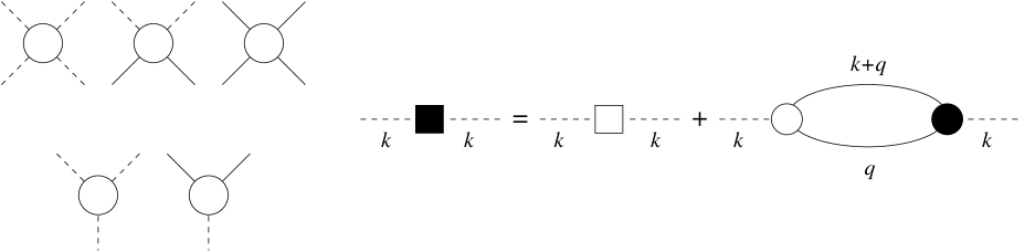
Figure 3: C. Di Castro, et al. - Renormalization group…

whence it is seen that the most singular contribution in the infrared is carried by $G_{TT}$. In the presence of the condensate, the four-leg vertex associated to the coupling constant $v$ yields various four- and three-leg vertices, associated to the various coupling constants $v_{LLLL}$, etc., $v_{LLL}$, etc. (see Fig. 3). Starting from Eq. (5), the dimensional analysis, in units such that $[q]=[\omega]=1$, identifies nine relevant or marginal running variables with singular corrections in $d\leq 3$.

However, the number of independent parameters is reduced by the exploitation of the local gauge invariance of the model. The free energy ${\cal F}$, or equivalently $\Gamma$, are invariant under the local transformation generated by the operator

$${\cal T}=\left[\begin{array}[]{cc}\cos\vartheta&-\sin\vartheta\\ \sin\vartheta&~{}~{}\cos\vartheta\end{array}\right]\simeq 1+\vartheta\left[\begin{array}[]{cc}0&-1\\ 1&~{}~{}0\end{array}\right],$$

which acts in the $L,T$ space, i.e.,

$$\Gamma[A_{\nu}+\partial_{\nu}\vartheta,{\cal T}_{ij}\varphi_{j0}]=\Gamma[A_{\nu},\varphi_{i0}],$$ (6)

with $i=L,T$ and $j=L,T$.

Functional derivatives of $\Gamma$ with respect to $\vartheta$, $A_{\nu}$, and $\varphi$ generate the various Ward identities. The first two are obtained by a functional derivativation with respect to $\vartheta$ and then either with respect to $\varphi_{L}$ or $\varphi_{T}$. In this way the Ward identities connect the two-point vertices to the external fields, showing, e.g., that when $h\rightarrow 0$ no gap is present in the spectrum. In this way the Hugenholtz-Pines theorem is simply recovered. Three-point vertices are related to two- and four-point vertices via three relations, which are the implementation of the continuity equation for this special case in the presence of the condensate. By then, all the strongly relevant coupling constants are fixed, and one is left with four marginal running variables. However, three of them are connected to physical quantities. In fact, they are related to the derivatives of the vertices with respect to frequency or momentum, and the corresponding Ward identities involve density and current correlation functions, thus implying relations to superfluid density, condensate compressibility, sound velocity, all of them free of divergences. Therefore, these identities guarantee the exact cancellation of the singular contributions in these variables, which are then RG invariants.

After all the identifications are made, one running variable is left, e.g., the longitudinal two-point vertex coupling $v_{LL}$.

The one-loop RG equations reproduce this situation of being left with only $v_{LL}$ as running coupling, with $v_{LL}\sim s^{\tilde{\epsilon}}$, with $\tilde{\epsilon}=3-d\geq 0$, at $d\leq 3$. In this case the anomalous self-energy $\bar{\Sigma}$ vanishes.

For $d>3$, instead, $v_{LL}=2\mu$ is finite, and the Bogoljubov result is recovered. In both cases, the spectrum is linear, leading to sound-like low-energy excitations. However this spectrum is realized in a completely different way in $d\leq 3$.

As in the Luttinger liquid for the one-particle Green’s function, the behavior $v_{LL}\sim s^{\tilde{\epsilon}}$ is fixed exactly by the Ward identities, which allow to close the (dominant part of the) equation for $v_{LL}$ (see Fig. 3) since the three-leg vertex $v_{TTL}$ is identified with $v_{LL}/\varphi_{L0}$ via Ward identities. When dealing with RG loop expansions, further corrections to the one-loop RG results cannot change the power-law exponents.

4 An example of unconventional criticality: the metal-insulator transition

4.1 Metal-insulator transition in disordered electron systems

When we deal with disordered electron systems, the singularities do not come directly from integrations of loops in terms of the original fermion propagators, as in Fig. 1, but rather from the soft collective modes related to diffusion, in terms of which an effective action can be derived for both non-interacting [59, 60] and interacting systems [28]. In this case, we will therefore enter in rather more details with respect to the previous topics.

According to basic quantum mechanics, within the one-electron approximation, insulating and metallic behavior occur as a result of the complete or partial filling of the highest occupied energy band of a solid, respectively. Beyond the one-electron approximation, correlation effects may lead to a drastic rearrangement of the energy levels and give rise to insulating behavior in situations where the metallic one is expected on the basis of band filling. This is usually referred to as a Mott phenomenon.

Scattering from randomly located impurities may also lead to a transition from a metallic to an insulating behavior. In this second case, rather than a rearrangement of the energy levels, the coherent scattering from the impurities modifies the phase of the electron wave function in such a way that it may result localized in space, thereby yielding an insulating behavior [61]. Experiments were performed both in metallic and semiconducting systems. These latter, in particular, turned out to be better suited for the study of the MIT, since the degree of disorder could be changed by the doping level, as it happens, for instance, in silicon doped with phosphorus (Si:P). There exist several review articles, which summarize the development of the field at various stages [10, 11, 12, 13, 14, 15, 16]. In recent years, there has been a renewed interest in the MIT, which is very actively investigated in the two-dimensional electron gas of MOSFET and heterostructure devices (for a recent review see, e.g., Ref. [62]).

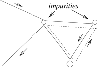
Figure 4: C. Di Castro, et al. - Renormalization group…

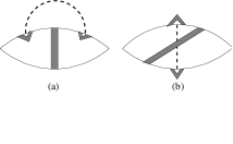
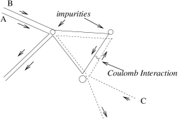
Figure 5: C. Di Castro, et al. - Renormalization group…

At theoretical level, a crucial element was the discovery that the quantum corrections to the classical Drude formula for the electrical conductivity give rise to singular terms in low-dimensional systems. These corrections arise as a result of the quantum interference of electron waves in disordered systems. There are two types of such terms. The first, known as the weak-localization (WL) correction, is a purely one-particle effect and is due to the interference of time reversed trajectories [63, 64] (see Fig. 4). The second is a consequence of the enhancement of the electron-electron interaction in a disordered system and is usually referred to as electron-electron interaction (EEI) correction [65, 66] (see Fig. 5).

In two dimensions, in particular, both the WL and the EEI correction to the conductivity are logarithmic,

$$\Delta\sigma_{\rm WL}=-{e^{2}\over\pi^{2}\hbar}\ln(L_{\phi}/l),$$ (7)

$$\Delta\sigma_{\rm EEI}=-{e^{2}\over\pi^{2}\hbar}\ln(L_{T}/l).$$ (8)

Both the above effects have been discussed in great detail in the literature and we do not provide a derivation of Eqs. (7,8) here, but limit ourselves to a comment on the EEI correction, after Eq. (12).

In Eqs. (7,8), the argument of the logarithmic corrections contains the ratio of two length scales. The first is the mean free path, $l=v_{F}\tau$, $\tau$ being the elastic scattering time, which sets the microscopic scale, beyond which the system behaves diffusively. The second length scale differs in the two cases. For WL it is $L_{\phi}$, the scale over which inelastic scattering starts to destroy the interference effects and one can show that it becomes infinite at zero temperature [67]. For EEI it is usually given by the thermal length $L_{T}$. In a diffusive system, all length scales correspond to characteristic times via the diffusion constant $D=v_{F}^{2}\tau/2$: the elastic scattering time $\tau=l^{2}/D$, the dephasing time $\tau_{\phi}=L^{2}_{\phi}/D$, and the thermal time $\tau_{T}=\hbar/k_{B}T=L^{2}_{T}/D$. As a result, the above corrections become singular at low temperature.

By recalling the Drude formula for the electrical conductivity $\sigma=2e^{2}N_{0}D$, where $N_{0}$ is the single-particle density of states at the Fermi level, one sees that the corrections (7,8) in units of $\sigma$ are controlled by the factor $t=1/(4\pi^{2}N_{0}D\hbar)$ (not to be confused with the deviation from the critical temperature of the previous sections). The parameter $t$ is related to the two-dimensional conductance $g=G/(e^{2}/h)$, by $t=1/(g\pi)$. In good metals, normally, $g\gg 1$ and $t$ is a small parameter.

The WL correction has been used to formulate a scaling theory of the MIT [59, 63] (for a pedagogical introduction see, e.g., Nagaoka’s and Kawabata’s contributions in Ref. [11]). This theory has a unique scaling variable, the dimensionless conductance $g$, which according to the Thouless’s argument describes how the eigenstates of the system change when we add together blocks of size $L$ to make blocks of size $2L$ [68]. There are two energy scales to be considered. The first is the energy level spacing that goes as $\Delta E=1/(dN/dE)=1/(N_{0}L^{d})$. The second is the energy perturbation due to the change in the boundary conditions. This may be related to the travel time in a diffusive system of size $L$, i.e., $\delta E\approx\hbar/\tau=\hbar\sqrt{D/L^{2}}$. The ratio of these two energies gives

$$\frac{\delta E}{\Delta E}=\frac{1}{2\pi}\frac{\sigma}{2e^{2}/h}L^{d-2}=\frac{g}{2\pi}.$$

Starting from the metallic side, where $\sigma$ is a constant, we see that in two dimensions the conductance $g$ becomes marginal. By assuming a scaling behavior, one can derive a RG flow equation for $g$ from the WL correction in Eq. (7). As a result one predicts that, in two dimensions, the RG flow drives the system to an insulating ground state, with $g\rightarrow 0$. The EEI shows qualitatively the same effect and one wonders whether one has to introduce further scaling parameters to take into account the interaction strength [69]. The answer to such a question is far from trivial and has required quite some work. In particular, it has been understood that, within a Fermi-liquid description, the Landau parameters provide the additional running variables whose RG flow has to be studied together with the conductance $g$ [28, 31]. In order to emphasize the physical origin of the additional running variables, we show in the next section how the interplay of interaction and disorder gives rise to singular corrections to thermodynamic quantities. This is to be contrasted with the WL correction which leaves the thermodynamic properties unaffected.

4.2 Thermodynamics

We present the derivation of the correction to the thermodynamic potential due to the interaction and disorder [30, 36, 70]. The coupling to the impurities is described by the Hamiltonian

$$H_{imp}=\int{\rm d}{\bf r}U({\bf r})\psi_{\alpha}^{\dagger}({\bf r})\psi_{\alpha}({\bf r}),$$

while the electron-electron interaction is of the standard form

$$H_{int}=\frac{1}{2}\int{\rm d}{\bf r}{\rm d}{\bf r}^{\prime}V_{0}({\bf r}-{\bf r}^{\prime})\psi_{\alpha}^{\dagger}({\bf r})\psi_{\beta}^{\dagger}({\bf r}^{\prime})\psi_{\beta}({\bf r}^{\prime})\psi_{\alpha}({\bf r}).$$

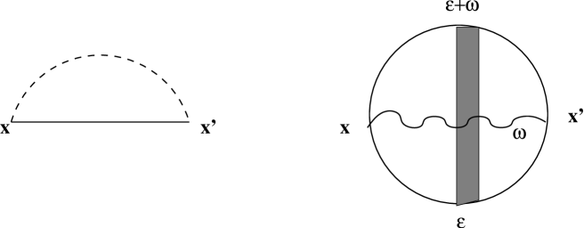
Figure 6: C. Di Castro, et al. - Renormalization group…

Greek indices indicate spin indices and sum over repeated indices is understood. To begin with, let us consider the first-order exchange-interaction correction to the thermodynamic potential (see Fig. 6)

$$\Delta\Omega=-\frac{1}{2}T^{2}\sum_{\omega,\varepsilon}\int{\rm d}{\bf r}{\rm d}{\bf r}^{\prime}V({\bf r}-{\bf r}^{\prime},\omega)G({\bf r},{\bf r}^{\prime};\varepsilon)G({\bf r}^{\prime},{\bf r};\varepsilon+\omega),$$ (9)

where we have introduced a retarded electron-electron interaction $V({\bf x}-{\bf x}^{\prime},\omega)$ to take into account screening effects which we will come back to later on. $\omega$ and $\varepsilon$ are Matsubara boson and fermion frequencies, respectively. Notice that the electron Green’s function depends separately on its spatial arguments, since translational invariance does not hold in the presence of disorder. In general, however, the impurities are randomly distributed and it is enough to average over them. For the average quantities the translational invariance is restored. The average can be performed by means of the well-known impurity technique[54]. In Eq. (9) this implies to average the product of the two Green’s functions. We assume a Gaussian, $\delta$-correlated impurity potential $U({\bf r})$ with

$$\langle U({\bf r})U({\bf r}^{\prime})\rangle={1\over 2\pi N_{0}\tau}\delta({\bf r}-{\bf r^{\prime}}),$$ (10)

and use a self-consistent Born approximation for the electron self-energy (see Fig. 6)

$$\Sigma({\bf r},t;{\bf r}^{\prime},t^{\prime}) = {1\over 2\pi N_{0}\tau}G({\bf r},t;{\bf r},t^{\prime})\delta({\bf r}-{\bf r}^{\prime}).$$ (11)

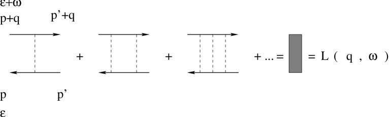
Figure 7: C. Di Castro, et al. - Renormalization group…

When the above self-energy is used to evaluate the Green’s function, one obtains a self-consistency equation which leads to a finite lifetime $\tau$. The average procedure is limited to correlations of impurity insertions according to Eq. (10). Insertions made on the same Green’s function are automatically taken into account in Eq. (11). When one has an average of two or more Green’s functions, as in evaluating the response functions, correlations between insertions on different Green’s functions must also be considered. To this end one re-sums the infinite series of the so-called ladder diagrams (see Fig. 7)

$$L({\bf q},\omega)=1+\eta+\eta^{2}+...=\frac{1}{1-\eta},$$

where

$$\eta=\frac{1}{2\pi N_{0}\tau}\sum_{\bf p}G({\bf p},\varepsilon)G({\bf p}+{\bf q},\varepsilon+\omega).$$

The sum over the momentum ${\bf p}$ differs from zero only when the Matsubara energies $\varepsilon$ and $\varepsilon+\omega$ have opposite signs. For vanishing frequency and momentum, $\eta\rightarrow 1$ signaling the emergence of a (diffusive) pole in the ladder. Indeed, in the low-frequency and momentum approximation, $\omega\tau\ll 1$ and $v_{F}q\tau\ll 1$, which defines the diffusive regime, the ladder sum reads

$$L({\bf q},\omega)=\frac{1}{2\pi N_{0}\tau^{2}}\frac{1}{Dq^{2}+|\omega|}.$$ (12)

The above equation is telling us that the two-particle propagation has a diffusive form. This means that, whereas the single-particle Green’s function is exponentially decaying over a mean free path, $l=v_{F}\tau$ ($v_{F}$ is the Fermi velocity), the collective density fluctuations propagate diffusively over large distances. It is the long-range diffusive character of the density fluctuations which is responsible of the logarithmic behavior of the EEI corrections to the conductivity and to the thermodynamic properties in two dimensions, as we are about to see. Technically, the logarithmic corrections arise from the integration over the diffusive pole. Each momentum integration, in two dimensions, yields a factor $1/D\sim t$, the expansion parameter. We would like to emphasize that the emergence of critical massless modes is highly non-trivial and shows how the construction of the effective action is in this case rather unconventional, to say the least.

The diffusive form of the two-particle propagator (usually called diffuson) makes the small-$q$ region more relevant. As a consequence, the Fourier transform of the interaction in Eq. (9) becomes important only for small momentum transfer, i.e., $V(q=0)$. On the other hand, the corresponding Hartree diagram contribution, after the average over the impurities, selects the interaction at large momentum transfer, i.e., $V(q=2p_{F})$.

The good-metal condition, $g\gg 1$, can be written in an equivalent form as $E_{F}\tau/\hbar\gg 1$, which implies that the disorder only affects states within a small shell $\hbar/\tau$ away from the Fermi surface. Under these circumstances, since disorder modifies only states near the Fermi surface, interaction effects at larger energy can be taken into account via the Fermi-liquid theory, which goes beyond the first-order perturbation theory in the interaction, by replacing $V(q=0)$ and $V(q=2p_{F})$ with the corresponding Fermi-liquid scattering amplitudes $\Gamma_{1}$ and $\Gamma_{2}$, whose lowest order diagrams are depicted in Fig. 8. Since, in the absence of spin-flip mechanisms, the total spin entering the two-particle propagator is a conserved quantity, it is convenient to introduce the singlet and triplet scattering amplitudes

$$\Gamma_{s}=\Gamma_{1}-\frac{1}{2}\Gamma_{2},~{}~{}~{}~{}~{}~{}~{}~{}\Gamma_{t}=\frac{1}{2}\Gamma_{2}.$$

We recall that the scattering amplitudes $\Gamma_{s}$ and $\Gamma_{t}$ are related to the Landau Fermi-liquid parameters $F_{s,a}^{0}$ which enter in the compressibility and spin susceptibility, by

$$\Gamma_{s}=\frac{1}{2N_{0}}\frac{F_{s}^{0}}{1+F_{s}^{0}},~{}~{}~{}~{}~{}~{}~{}~{}\Gamma_{t}=-\frac{1}{2N_{0}}\frac{F_{a}^{0}}{1+F_{a}^{0}}.$$

From now on, when necessary, $N_{0}$ is assumed to include the Landau effective-mass correction. The scattering amplitudes are dynamically screened by the diffusive density fluctuations, leading to dressed scattering amplitudes

$$\Gamma_{s,t}(q,\omega)=\Gamma_{s,t}\frac{Dq^{2}+|\omega|}{Dq^{2}+(1\mp 2N_{0}\Gamma_{s,t})|\omega|}.$$

However, this dressing does not alter the degree of divergence of a given diagram.

We are now ready to present the expression for the correction to the thermodynamic potential. By means of the previous substitutions, this is obtained to all orders in the interaction, but to first order in the expansion parameter $t$. It is convenient to use the standard trick [71] of multiplying the interaction by a parameter $\lambda$ and integrating over it between $0$ and $1$. We then get

$$\Delta\Omega= - T\sum_{q\omega}\int_{0}^{1}{\rm d}\lambda\left[\frac{N_{0}\Gamma_{s}|\omega|}{Dq^{2}+(1-\lambda 2N_{0}\Gamma_{s})|\omega|}\right.$$

$$- \left.\sum_{M}\frac{{N_{0}\Gamma}_{t}|\omega|}{Dq^{2}+(1+\lambda 2N_{0}\Gamma_{t})|\omega|-{\rm i}M(1+2{N_{0}\Gamma}_{t})\omega_{s}{\rm sgn}(\omega)}\right].$$

To allow for the calculation of the spin susceptibility, in the above equation we have introduced also a magnetic field via the Zeeman coupling, $\omega_{s}=g\mu_{B}B$ and $M$ labels the triplet states. Notice the introduction of the Fermi-liquid renormalization of the Zeeman energy [72]. After evaluating the integrals one gets

$$\Delta\Omega=\Delta\Omega_{0}+\Delta\Omega_{1}+tN_{0}T^{2}\Delta\Omega_{2}\left(\frac{\omega_{s}}{T}\right)$$ (13)

where

$$\Delta\Omega_{0} = -tN_{0}T^{2}(2N_{0}\Gamma_{s}-6{N_{0}\Gamma}_{t})\left(\frac{\pi^{2}}{6}\ln(T\tau)+A\right),$$

$$\Delta\Omega_{1} = tN_{0}{N_{0}\Gamma}_{t}(1+2{N_{0}\Gamma}_{t})\omega_{s}^{2}\ln(\omega_{s}\tau),$$

$$\Delta\Omega_{2}(x) = (1+2{N_{0}\Gamma}_{t})I(x)-I((1+2{N_{0}\Gamma}_{t})x)-4A{N_{0}\Gamma}_{t},$$

$$I(x) = \int_{0}^{\infty}{\rm d}yb(y)\left[(y-x)\ln|y-x|+(y+x)\ln|y+x|\right],$$ (14)

where $b(x)$ is the Bose function and $A\approx-0.24$. Eqs. (13,14) are organized to show the zero- and the large-magnetic-field behaviors, which are connected by the crossover function $\Delta\Omega_{2}(x)$. Notice that at small $x$, one has $\Delta\Omega_{2}(x)\approx-{N_{0}\Gamma}_{t}(1+2{N_{0}\Gamma}_{t})x^{2}\ln x$. As a result, the corrections to the specific heat and to the spin susceptibility read

$$\delta C_{V} = C_{V,0}t(N_{0}\Gamma_{s}-3{N_{0}\Gamma}_{t})\ln(T\tau),$$

$$\delta\chi = -\chi_{0}4t{N_{0}\Gamma}_{t}(1+2{N_{0}\Gamma}_{t})\ln(T\tau),$$ (15)

where $C_{V,0}=2\pi^{2}N_{0}T/3$ and $\chi_{0}=N_{0}(g\mu_{B})^{2}/2$ are the non-interacting values. We note that there is no dependence on the chemical potential implying that there are no singular corrections to the static compressibility $\partial n/\partial\mu$, i.e., $\delta(\partial n/\partial\mu)=0$. As a result, the compressibility has the Landau value

$$\frac{\partial n}{\partial\mu}=N_{0}\left(1-2N_{0}\Gamma_{s}\right)\equiv N_{0}Z_{s}^{0}.$$ (16)

Eq.(15) contains the leading divergent perturbative terms to thermodynamic properties of a disordered Fermi liquid. Before proceeding to the next sections, where we discuss the renormalized perturbation theory and how to obtain the equations for the RG flow including transport properties, we remark that in various physical systems the above corrections can actually be observed already in the metallic phase, where they are still within the reach of perturbation theory [13].

4.3 Ward identities and renormalized Fermi liquid

In order to get the RG equations, one has to absorb the logarithmic corrections in terms of the renormalization of a set of running variables. This is usually done in terms of the relevant parameters of the Hamiltonian. The difficulty of the problem at hand is precisely the fact that the effective Hamiltonian is not simply related to the microscopic one we started from. We have seen in the previous section that the logarithmic correction originates from an integration over the collective diffusive density modes. The propagator of the diffusive mode, which we have called ladder, is the result of a re-summation of impurity scattering to all orders. If we are going to obtain a renormalized theory, we must understand how the logarithmic correction we have obtained in the previous section will manifest in the effective field theory for the diffusive modes. This task can actually be carried out systematically from the outset by deriving a matrix-field non-linear $\sigma$-model [28]. This approach, however, makes the connection with the physical quantities less direct. By the use of the Ward identities, all the renormalizations required by the non-linear $\sigma$-model are expressed through the Landau parameters, thus showing that the disordered interacting electron system can be effectively described by a scale-dependent Landau Fermi-liquid theory [29, 31, 36, 37, 73]. For this reason, we adopt here the approach of perturbation theory combined with the Ward identities.

We begin by recalling the expression of the density and current in linear response regime

$$j_{\mu}(\omega,{\bf q})=K_{\mu\nu}(\omega,{\bf q})A_{\nu}(\omega,{\bf q}),$$

where $j_{\mu}=(\rho,{\bf j})$ and $A_{\mu}=(\phi,{\bf A})$. $K_{\mu\nu}$ is the standard response function for density and current. In particular the conductivity and the compressibility are given by

$$\sigma = -\lim_{\omega\rightarrow 0}\frac{{\rm Im}K}{\omega},$$

$$\frac{\partial n}{\partial\mu} = -\lim_{{\bf q}\rightarrow 0}K_{00}(0,{\bf q}),$$

where $K=(1/d)\sum_{1,d}K_{ii}$, assuming spatial isotropy. In a similar way, one defines the spin-spin $\chi(\omega,{\bf q})$ and energy-energy $\chi_{E}(\omega,{\bf q})$ response functions, whose static limit (i.e., $\omega\rightarrow 0$ first, ${\bf q}\rightarrow 0$ after) are the spin susceptibility and the specific heat times the temperature.

The global conservation law and gauge invariance give rise to the following Ward identities

$$q_{\mu}K_{\mu\nu} = 0,$$

$$K_{\mu\nu}q_{\nu} = 0,$$ (17)

that must be obeyed to all orders in perturbation theory. Notice that the first equation is nothing but a different way of writing Eq. (1). For instance, a disordered non-interacting Fermi system has a density-density response function given by

$$K_{00}=-\frac{\partial n}{\partial\mu}\frac{Dq^{2}}{Dq^{2}-{\rm i}\omega}=-\frac{\partial n}{\partial\mu}-\frac{{\rm i}\omega N_{0}}{Dq^{2}-{\rm i}\omega},$$

The first expression is nothing but a statement about the diffusive nature of the density fluctuations. The second expression, which separates the so-called dynamic part of the response function, is the result of a direct diagrammatic calculation. To understand this point, recall that the evaluation of the bubble-like diagram involves an integral over the energy of a product of two Green’s functions. The dynamic part corresponds to the energy range where the two Green’s functions have poles on opposite sides of the real axis, in the complex plane, and a ladder resummation can be performed. $N_{0}$ appears since we are dealing with a non-interacting system. From Eqs. (17), it follows that

$$K_{00}(\omega,0)=0,$$ (18)

which immediately gives that the compressibility $\partial n/\partial\mu$ coincides with the single-particle density of states, as it is expected for the non-interacting system. The single-particle density of states, furthermore, may be generally related to the dynamic part of the response function $K^{+-}_{00}$, i.e.,

$$K^{+-}_{00}=-{\rm i}\int_{-\omega}^{0}\frac{{\rm d}\varepsilon}{2\pi}\sum_{\bf p}G({\bf p},\varepsilon)G({\bf p}+{\bf q},\varepsilon+\omega)\Lambda_{0}^{+-}({\bf p},{\bf q},\varepsilon,\omega),$$ (19)

where $\Lambda_{0}^{+-}$ is the density vertex in the energy range $\epsilon(\epsilon+\omega)<0$, which in the non-interacting case gives the total dynamic part of the response function. The reason for defining the vertex $\Lambda_{0}^{+-}$ in this energy range is due to the possibility of inserting the ladder resummation. For positive external frequency $\omega$, the energy restriction determines the integration range over the energy $\epsilon$ in Eq. (19). By using the general Ward identity Eq. (1), in the dynamic limit, one gets the single-particle density of states

$$N\equiv-\frac{1}{\pi}\sum_{\bf p}{\rm Im}G({\bf p},\varepsilon={\rm i}0^{+})=\lim_{\omega\rightarrow 0}\lim_{{\bf q}\rightarrow 0}K^{+-}_{00}(\omega,{\bf q}).$$ (20)

In the simple non-interacting case, of course, $N=N_{0}$.

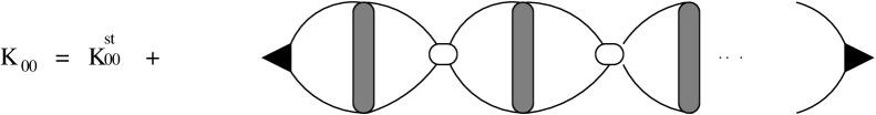
Figure 9: C. Di Castro, et al. - Renormalization group…

We stress that both Eqs. (18,20) are always valid and we use them in the following when dealing with interacting electrons. Here, they will allow us to control the logarithmic corrections which arise from the interplay between the diffusive motion of the electrons and their mutual interaction. We refer to renormalized quantities with a bar. The diagrammatic skeleton structure of the response function is shown in Fig. 9. $\Lambda_{s}$ is, in the interacting case, the vertex which, when multiplied by $K_{00}^{+-}$ gives the total dynamic part of $K_{00}$, which includes also terms ending with two advanced ($++$) or retarded ($--$) Green’s functions[37]. A direct perturbative evaluation of the density response function gives

$${\bar{K}}_{00}^{+-}=-\frac{{\rm i}\omega N_{0}\zeta^{2}\Lambda_{s}}{{\bar{D}}q^{2}-{\rm i}\omega Z_{s}},~{}~{}~{}~{}~{}~{}~{}~{}{\bar{K}}_{00}=-\overline{\frac{\partial n}{\partial\mu}}+{\bar{K}}_{00}^{+-}\Lambda_{s}$$ (21)

where

$$Z_{s}\equiv Z-2N_{0}\zeta^{2}{\bar{\Gamma}}_{s}$$ (22)

is the renormalized form of $Z_{s}^{0}$, defined in Eq. (16), and the singular corrections have been absorbed in the renormalized quantities ${\bar{D}}$, $Z$, $\zeta$, ${\bar{\Gamma}}_{s}$ and $\Lambda_{s}$. The first three are obtained by considering the corrections to the ladder in the presence of interaction. ${\bar{\Gamma}}_{s}$ is the renormalized scattering amplitude in the singlet channel.

Here, the parameter $\zeta$ plays the role of the wave-function renormalization of the effective field theory with the ladder as a propagator, while $Z$ renormalizes the frequency, and it will be identified with the specific heat renormalization parameter. By the use of Ward identities we now show that $\zeta$ also coincides with the renormalization of the single-particle density of states introduced by the disorder, in the presence of the interaction, i.e.,

$$N=\zeta N_{0}.$$ (23)

Indeed, when Eqs. (18,20) are used in Eq. (21), we obtain

$$\frac{N}{N_{0}}=\frac{\zeta^{2}\Lambda_{s}}{Z_{s}},~{}~{}~{}~{}~{}~{}~{}~{}\overline{\frac{\partial n}{\partial\mu}}=N_{0}\frac{\zeta^{2}\Lambda_{s}^{2}}{Z_{s}}.$$ (24)

Since the compressibility has no singular corrections, $Z_{s}$ coincides with $Z_{s}^{0}$ and $\zeta\Lambda_{s}=Z_{s}^{0}$, whence Eq. (23) follows. Thus, the single-particle density of states becomes scale-dependent, in contrast to the non-interacting case.

In a similar way, considering $Z_{t}=Z-2N_{0}\zeta^{2}\bar{\Gamma}_{t}$, one obtains for the specific heat and for the spin susceptibility the relations

$${\bar{C}}_{V} = ZC_{V},$$

$${\bar{\chi}} = Z_{t}N_{0}.$$ (25)

The above equations relate the renormalization parameters $Z$, and $Z_{t}$ that appear in the perturbative correction to the physical quantities $C_{V}$ and $\chi$. Contrary to $Z_{s}$, $Z$ and $Z_{t}$ are affected by logarithmic singularities, which can be derived through the evaluation of the thermodynamic potential. Alternatively, one can compute the corrections to $Z$, and $Z_{t}$ directly (although with a lot more effort) in perturbation theory and find a perfect agreement between the expressions obtained via the thermodynamic potential and Eqs. (25).

Before going to the next section, to deal with the RG equations, we would like to recall the complete expression for the electrical conductivity. To do so, we notice that in the presence of Coulomb long-range forces, to avoid double counting, one has to subtract the statically screened long-range Coulomb $\Gamma_{0}$ from the full singlet scattering amplitude entering the ladder resummation for the density-density response function. Hence, ${\bar{\Gamma_{s}}}\rightarrow{\bar{\Gamma_{s}}}-\Gamma_{0}$, Eq.(22) for $Z_{s}$ is modified accordingly, and $\Gamma_{0}$ reads

$$\Gamma_{0}(q,\omega=0) = \frac{V_{C}(q)\Lambda_{s}^{2}}{1+V_{C}(q)2{\bar{\partial n/\partial\mu}}}\rightarrow_{q\rightarrow 0}\frac{\Lambda_{s}^{2}}{2{\bar{\partial n/\partial\mu}}}.$$ (26)

As a consequence, by using Eq.(24), we derive the constraint

$$Z=2N_{0}\zeta^{2}{\bar{\Gamma}}_{s}.$$ (27)

Then the EEI correction to the conductivity by including also the effect of the triplet channel and of the dynamical re-summation [28, 31] becomes

$$\delta t=-t^{2}\left[1+3\left(1-\frac{(1+2{\gamma}_{t})}{2{\gamma}_{t}}\ln(1+2{\gamma}_{t})\right)\right]\ln(T\tau),$$ (28)

where $N_{0}\zeta^{2}{\bar{\Gamma}_{t}}/Z=\gamma_{t}$. The first term in the square brakets is the contribution due to the singlet channel in the presence of long-range Coulomb interaction [see Eq. (8)]. Notice that the corresponding scattering amplitude does not appear explicitly, due to the constraint (27). An analogous contribution would come from the WL correction, given by Eq. (7). This last term, together with the contribution of the interaction in the particle-particle channel, is here suppressed to maintain the discussion simple while keeping all the general features of the theory.

Finally, we would like to remark about the various “density of states” we have encountered. We have the thermodynamic density of states or compressibility $\partial n/\partial\mu$, the coefficient of the linear-in-$T$ term of the specific heat, $\gamma$, and the single-particle density of states obtained from the Green’s function, $N$. In the non-interacting case all these quantities, together with the spin susceptibility, coincide with $N_{0}$, but in the presence of interaction and disorder they are renormalized by $Z_{s}$, $Z$, $\zeta$, and $Z_{t}$, respectively. The Ward identities are a very powerful tool in controlling the different role played by these quantities in the renormalized theory.

4.4 One-loop RG equations for the renormalized Fermi liquid

In the previous section we have seen that all the divergences which appear in perturbation theory may be absorbed into the renormalization of the physical parameters characterizing a Fermi liquid. Therefore, we can use the previous results to obtain here the RG flow equations for $Z=C_{V}/C_{V,0}$ and $Z_{t}/Z=\chi/Z\chi_{0}$. From Eqs. (15,28), introducing the scaling variable $s=-\ln(T\tau)$, one gets [28, 31, 32, 34, 37]

$$\left\{\matrix{\displaystyle{\frac{{\rm d}Z}{{\rm d}s}}&=&\displaystyle{-\frac{tZ}{2}(1-6{\gamma}_{t}),~{}~{}~{}~{}~{}~{}~{}~{}~{}~{}~{}~{}~{}~{}~{}~{}~{}~{}~{}~{}~{}~{}~{}~{}~{}~{}~{}~{}~{}~{}~{}~{}~{}~{}~{}~{}~{}~{}~{}~{}~{}~{}~{}}\cr\displaystyle{\frac{{\rm d}{\gamma}_{t}}{{\rm d}s}}&=&\displaystyle{\frac{t}{4}(1+2{\gamma}_{t})^{2},~{}~{}~{}~{}~{}~{}~{}~{}~{}~{}~{}~{}~{}~{}~{}~{}~{}~{}~{}~{}~{}~{}~{}~{}~{}~{}~{}~{}~{}~{}~{}~{}~{}~{}~{}~{}~{}~{}~{}~{}~{}~{}~{}~{}}\cr\displaystyle{\frac{{\rm d}t}{{\rm d}s}}&=&\displaystyle{-\epsilon\frac{t}{2}+t^{2}\left[1+3\left(1-\frac{(1+2{\gamma}_{t})}{2{\gamma}_{t}}\ln(1+2{\gamma}_{t})\right)\right],}}\right.$$ (29)

where the last equation is derived through Eq. (28), considering the bare dimension $\epsilon=d-2$ of the coupling $t$ in units of inverse length. We briefly review the main consequences of the above equations. Let us begin the discussion in two dimensions, i.e., $\epsilon=0$ (see Fig. 10). Under the RG, ${\gamma}_{t}$ grows always and diverges at a finite scale. In the equation for $t$ the singlet contribution makes it larger (localizing character), whereas the triplet contribution (in the round brackets) does the opposite (antilocalizing). If the initial value of ${\gamma}_{t}$ is not too large, $t$ initially grows until the growth of ${\gamma}_{t}$ makes the triplet contribution the dominating one. As a result, $t$ has a maximum as a function of $s$. However, due to the strong-coupling runway of ${\gamma}_{t}$, one cannot seriously trust the above equations quantitatively. Nevertheless, the physical indication of some type of ferromagnetic instability is rather clear due to the diverging spin susceptibility associated with $\gamma_{t}$. Furthermore, the dominating antilocalizing effect of the triplet while $t$ remains finite, strongly supports the possibility of a metallic phase at low temperature, in contrast with the non-interacting theory based on WL only [32, 34, 37, 38, 39]. Indeed, this metallic phase in $d=2$ has been recently observed (See Refs. in [62]). In addition, due to the divergence of $\gamma_{t}$ also $Z$ goes to the strong coupling regime, leading to an enhancement of the specific heat, which is however hardly observable in two dimensions.

In three dimensions (see Fig. 11) one has a richer scenario depending on the initial values of the running couplings. The main difference is that there exists a critical line in the $t-\gamma_{t}$ plane asymptotically given by $t\gamma_{t}=\epsilon/2$, where under the RG flow $t\rightarrow 0$, $\gamma_{t}\rightarrow\infty$ with their product being constant. On the weak-disorder side of this line, the system scales to a conductor with vanishing $t$, whereas on the strong-disorder side the system behaves qualitatively as in the two-dimensional case discussed above, leaving again the possibility open for a ferromagnetic instability at a finite scale. In this latter case, however, the strong-coupling runaway flow requires to go beyond the one-loop approximation we have presented here leaving the problem of the proper treatment of the metal-insulator transition still open. An approximate treatment of the two-loop correction is possible, but its discussion is well outside the scope of this paper. We refer the reader to Ref. [15]. However, we remark that, whenever there is a reduction of the effect of the triplet channel, due to a magnetic coupling altering the symmetry, as in the presence of a magnetic field with Zeeman spin-splitting [31, 35], spin-flip scattering[29, 31, 35] or spin-orbit scattering [29, 33] one obtains a bona-fide MIT with different universality classes with respect to the Anderson localization. For a comparison with the experiments see, e.g., Ref. [74].

We finally emphasize that, as in the interacting boson case, the perturbative RG at one loop confirms the conclusions drawn by the implementation of the Ward identities. However, in the present case, since we are dealing with critical behavior, the singularities are resummed in power laws, rather than to be cancelled as required in a stable liquid phase. Mathematically this manifests in the lack of additional symmetries which prevents us from closing the equations of motion and solving the problem exactly. We have achieved, however, via the Ward identities, that the remaining singularities describe the critical behavior of the specific heat, spin susceptibility, and of the coupling $t$ related to the conductance.

Acknowledgments. S. C. and C. D. C. acknowledge financial support from the Italian MIUR, Cofin 2001, prot. 20010203848, and from INFM, PA-G0-4. R. R. acknowledges partial financial support from E.U. by Grant RTN 1-1999-00406, and from the Italian MIUR, Cofin 2002.

Table captions

Tab. 1. In the table we give a summary of the conservation laws exploited in order to keep under control the singularities arising in perturbation theory, for each of the physical systems discussed in the text. In particular, we indicate the conservation laws (second column), the practical consequence of their implementation (third column), the behavior of the system (fourth column), and the equation number where the corresponding Ward identity can be found in the article (fifth column).

Physical System	Conservation Law	Consequence	Behavior	Ward Identity
Interacting Fermions	Global and separate Left and Right number density	Cancellation of singularities in correlation functions	Unusual non-critical	Eqs. (1,2)
Interacting Bosons	Global number density and $U(1)$-gauge invariance	Identification and reduction of running variables	Unusual non-critical	Eq. (6)
Disordered Interacting Electrons	Global number density and $U(1)$-gauge invariance	Identification and reduction of running variables	Critical	Eqs. (1,17)

Table 1: C. Di Castro, et al. - Renormalization group…

Figure captions

Fig. 1. (a): Lowest-order correction to the coupling constant of the $\varphi^{4}$ theory. Each line in the loop carries a factor $[t+{\bf q}^{2}]^{-1}$, and an integral over $d^{d}{\bf q}$ is implied, giving a contribution which diverges as $|t|^{-\epsilon/2}$ for $t\to 0$, when $\epsilon>0$, i.e., $d<4$. The divergence is logarithmic for $\epsilon=0$ ($d=4$). (b): Lowest-order correction to the coupling constant of an interacting Fermi system. Each line in the loop carries a factor $[\varepsilon-v_{F}(|{\bf p}|-p_{F})]^{-1}$, where $v_{F}$ is the Fermi velocity and $p_{F}$ the Fermi momentum, and an integral over $d\varepsilon d^{d}{\bf p}$ is implied, giving a logarithmic divergence in the external momentum or frequency, when $d=1$. (c): The four-point vertex of an interacting Bose systems generates also two- and three-leg vertices below the condensation temperature. The dashed line represents a condensed boson. (d): Lowest-order correction to the single-particle propagator of an interacting Bose system, associated with three-leg vertices below the condensation temperature. Each line in the loop carries a factor $[\omega^{2}-c^{2}{\bf q}^{2}]^{-1}$, and an integral over $d\omega d^{d}{\bf q}$ is implied, giving a divergence as $s^{-\tilde{\epsilon}}$, where $s$ is a finite external momentum or frequency, for $\tilde{\epsilon}>0$, i.e., $d<3$. The divergence is logarithmic for $\tilde{\epsilon}=0$ ($d=3$).

Fig. 2. Dyson equation for the electron Green’s function $G$ (thick solid line). The thin solid line represents the bare Green’s function $G_{0}$, the tick-dashed line is the effective interaction $D$ (dressed by the RPA series), and the black triangle represents the irreducible scalar vertex $\Lambda_{0}$.

Fig. 3. Left: Various four- and three-leg vertices arising in the broken-symmetry phase. Dashed and solid lines represent longitudinal ($L$) and transverse ($T$) modes, respectively. Right: Equation for the most singular part of the two-point vertex $v_{LL}$ (filled square). The empty square represents the bare vertex $v_{LL}^{0}$, whereas the empty and black circles represent the three-leg vertices $v_{LTT}^{0}$ (bare) and $v_{LTT}$ (dressed), respectively. The external dashed lines, which represent longitudinal fluctuations, are amputated, and are only drawn to indicate the corresponding ingoing and outgoing momenta. The solid line represent the propagator of transverse fluctuations, $G_{TT}$. Notice that the perturbative one-loop RG equation for $v_{LL}$ is obtained by taking the bare vertices only.

Fig. 4. Left: Diagram giving the WL correction to the conductivity, Eq. (7). The dashed line represents the average of two impurity insertions, introduced later on in the text, Eq. (10). In general, it is necessary to sum up diagrams with an infinite number of impurity lines. The leading term gives rise to the ladder diagram explained in the text [cf. Eq. (12), see also Fig. 7]. In the case of electrical conductivity, one can show that this leading term reproduces the semiclassical result of the Drude-Boltzmann theory. The next correction is obtained by considering the series of maximally crossed ladder diagrams shown here. In Ref. [64], it has been shown that the crossed ladder may be evaluated in terms of the direct ladder by exploting the time reversal symmetry. Notice that, because of the crossing of all the impurity lines, the impurities visited by the top Green’s function line are met in reversed order by the bottom one. This is the diagrammatic representation of the interference of time-reversed trajectories. Right: The WL correction due to the interference by pairs of trajectories, one the time reversed of the other, is shown in a more pictorial way. In the figure, the two trajectories (solid and dashed lines) differ in the way one goes around the closed loop.

Fig. 5. Left: After non-trivial cancellations, as explained in Ref. [66], the diagrams (a) and (b) are those responsible for the EEI correction to the conductivity, Eq. (8). The diagrams shown here contribute to the singlet channel. Another set of diagrams, not shown here, may be obtained by considering the Hartree-like contributions. This latter set of diagrams gives rise to the correction to the conductivity in the triplet channel. In the figure, the tick dashed line represents the electron-electron interaction and the shaded parts the insertions of the infinite series of ladder diagrams[ see also Fig. 7]. Right: A physical picture of the processes taken into account by the diagrams on the left. Two trajectories (A and B) that differ by a closed loop do not, in general, interfere. The electron-electron interaction, however, may lead to interference, since the extra phase gained in the closed loop may be canceled by another electron (C) going around the same closed trajectory.

Fig. 6. Left: Self-energy in the Born approximation. The dashed line represents the average of two impurity insertions, Eq. (10). When the internal Green’s function (solid line) is replaced with the dressed Green’s function one obtains the self-consistent Born approximation. Right: First-order correction to the thermodynamic potential (exchange term). Upon impurity averaging, the ladder re-summation appears, which corresponds to repeated independent scattering events (see Fig. 7)

Fig. 7. The diagrammatic series of repeated impurity scattering. The dashed line represents the average over the impurity strength distribution. Physically, both the top (electron) and bottom (hole) Green’s function lines visit the same impurity site. Notice that, since the impurity scattering is elastic, the energy is not changed along an electron line. The infinite series of ladder diagrams is indicated with a shaded rectangle.

Fig. 8. Lowest order diagrams for small ($\Gamma_{1}$) and large ($\Gamma_{2}$ ) momentum transfer (scattering angle).

Fig. 9. Skeleton diagram of the response function. The black triangles represent the vertex $\Lambda_{s}$, the open squares the scattering amplitudes $\Gamma_{s,t}$, and the shaded rectangle the ladder of impurity lines, Eq. (12). $K_{00}^{st}$ is the static limit of the response function, i.e., the compressibility.

Fig. 10. RG flow corresponding to the equations (29), for $d=2$ ($\epsilon=0$), with $\gamma\equiv\gamma_{t}$. $\gamma/(1+\gamma)$ is plotted as a function of $t/(1+t)$ to transform the interval $[0,+\infty)$ into the interval $[0,1]$ on both axes. Observe that $\gamma_{t}$ always scales to strong coupling, i.e., $\gamma/(1+\gamma)\to 1$.

Fig. 11. RG flow corresponding to the equations (29), for $d=3$ ($\epsilon=1$). The notations are the same as in Fig. 10. Observe the two possible asymptotic behaviors: on the weak-disorder side (small $t$), $\gamma$ scales to a finite value, whereas a two-dimensional-like behavior, with $\gamma\to\infty$, is found on the strong-disorder side (large $t$). The separatrix is marked by a thicker line.

Figure 1: C. Di Castro, et al. - Renormalization group…

Figure 2: C. Di Castro, et al. - Renormalization group…

Figure 8: C. Di Castro, et al. - Renormalization group…

Figure 10: C. Di Castro, et al. - Renormalization group…

Figure 11: C. Di Castro, et al. - Renormalization group…

References

- [1] M. Gell-Man and F. E. Low, Phys. Rev. 95, 1300 (1954); N. N. Bogoliubov and P. V. Shirkov, Introduction to the theory of quantized fields, Intersciences Publishers, New York (1959); V. L. Bonch-Bruevich and S. V. Tyablikov, The Green’s function method in statistical mechanics, North-Holland Publishing Company, Amsterdam(1962).
- [2] K. G. Wilson, Phys. Rev. B 4, 3174 (1971); ibid., 3184 (1971).
- [3] See, e.g., Proceedings of the International School of Physics ‘Enrico Fermi’, Course LI, edited by M. S. Green’s, Academic Press, New York (1971).
- [4] K. G. Wilson and J. Kogut, Phys. Rep. C 12, 75 (1974).
- [5] A general overview and references are found, e.g., in Phase transitions and critical phenomena, vol. VI, edited by C. Domb and M. S. Green, Academic Press, New York (1976).
- [6] K. S. Ma, Modern theory of critical phenomena, W. A. Benjamin, Reading (1976); A. Z. Patašinskij and V. L. Pokrovskij, Fluctuation theory of phase transitions, Pergamon Press, Oxford (1979).
- [7] C. Di Castro and G. Jona-Lasinio, Phys. Lett. A 29, 322 (1969).
- [8] A.I. Larkin and D.E. Khmel’nitskii Zh. Eksp. Teor. Fiz. 56 2087 (1969)[Sov. Phys. JETP 29,1123 (1969)].
- [9] L. D. Landau, Sov. Phys. JETP 7, 19 (1937).
- [10] B. L. Altshuler, A. G. Aronov, D. E. Khmel’nitskii, and A. G. Larkin, in Quantum Theory of Solids, edited by I. M. Lifshitz, MIR Publishers, Moscow (1982); B. L. Altshuler and A. G. Aronov, in Electron-Electron Interactions in Disordered Systems, edited by M. Pollak and A. L. Efros, North-Holland, Amsterdam (1985), p. 1; P. A. Lee and T. V. Ramakrishnan, Rev. Mod. Phys. 57, 287 (1985).
- [11] See, e.g., Progr. Theor. Phys. Suppl. 84, 1-295 (1985), edited by Y. Nagaoka.
- [12] C. Castellani and C. Di Castro, in Applications of Field Theory to Statistical Mechanics, edited by L. Garrido, Springer-Verlag (1985).
- [13] See, e.g., Anderson Localization, Proceedings of the International Symposium, Tokio, Japan August 16-18, 1987, edited by T. Ando and H. Fukuyama, Springer-Verlag (1987).
- [14] A. M. Finkel’stein, in Electron Liquid in Disordered Conductors, edited by I. M. Khalatnikov, Soviet Scientific Reviews Vol. 14, Harwood, London (1990).
- [15] D. Belitz and T. R. Kirkpatrick, Rev. Mod. Phys. 66, 261 (1994).
- [16] See, e.g., Proceedings of the International Conference LOCALIZATION 1999: Disorder and Interaction in Transport Phenomena, Ann. Phys. (Leipzig) 8, (1999), edited by M. Schreiber Chemnitz.
- [17] J. Sólyom, Adv. Phys. 28, 201 (1979).
- [18] S. Beliaev, Sov. Phys. JETP 7, 289 (1958).
- [19] J. Gavoret and P. Nozières, Ann. Phys. (N.Y.) 28, 349 (1964).
- [20] I. E. Dzyaloshinski and A. I. Larkin, Sov. Phys. JETP 38, 202 (1974).
- [21] C. Di Castro and W. Metzner, Phys. Rev. Lett. 67, 3852 (1991); W. Metzner and C. Di Castro, Phys. Rev. B 47, 16107 (1993).
- [22] C. Castellani, C. Di Castro, and W. Metzner, Phys. Rev. Lett. 72, 316 (1994).
- [23] W. Metzner, C. Castellani, and C. Di Castro, Adv. Phys. 47, 317 (1998).
- [24] P. Bares and X. G. Wen, Phys. Rev. B 48, 8636 (1993); C. Castellani and C. Di Castro, Physica C 235-240, 99 (1994)
- [25] C. Castellani, S. Caprara, C. Di Castro, and A. Maccarone, Nucl. Phys. B 594, 747 (2001).
- [26] F. Pistolesi, Ph.D. thesis, Scuola Normale Superiore, Pisa (1996); C. Castellani, C. Di Castro, F. Pistolesi, and G. C. Strinati, Phys. Rev. Lett. 78, 1612 (1997); F.Pistolesi, C. Castellani, C. Di Castro, and G. C. Strinati, to be published.
- [27] G. Benfatto, in Constructive results in field theory, statistical mechanics, and condensed matter physics, edited by V. Rivasseau, Springer-Verlag, Berlin (1994).
- [28] A.M. Finkel’stein, Sov. Phys. JETP 57, 97 (1983).
- [29] B. L. Altshuler and A. G. Aronov Solid State Commun. 46, 429 (1983).
- [30] B. L. Altshuler, A. G. Aronov, and A. Yu. Zyuzin, Sov. Phys. JETP 57, 889 (1983).
- [31] C. Castellani, C. Di Castro, P.A. Lee, and M. Ma, Phys. Rev. B 30, 527 (1984).
- [32] C. Castellani, C. Di Castro, G. Forgacs S. Sorella Solid State Communications 52, 261 (1984).
- [33] C. Castellani, C. Di Castro, P. A. Lee, M. Ma, S. Sorella, and E. Tabet, Phys. Rev. B 30, 1596 (1984).
- [34] A. M. Finkel’stein, Z. Phys. 56, 189 (1984).
- [35] A. M. Finkel’stein, Zh. Eksp. Teor. Fiz.86 , 367 (1984) [Sov. Phys. JETP 59212,(1984).
- [36] C. Castellani and C. Di Castro, Phys. Rev. B 34, 5935 (1986).
- [37] C. Castellani, C. Di Castro, P. A. Lee, M. Ma, S. Sorella, and E. Tabet, Phys. Rev. B 33, 6169 (1986).
- [38] C. Castellani, C. Di Castro, and P. A. Lee, Phys. Rev. B 57, 9381 (1998).
- [39] A. Punnoose and A. M. Finkel’stein, Phys. Rev. Lett. 88, 016802 (2002).
- [40] A. Z. Patašinskij and V. L. Pokrovskij, Sov. Phys. JETP 19, 677 (1964); ibid. 23, 292 (1966).
- [41] L. P. Kadanoff, W. Götze, D. Hamblen, R. Hecht, E. A. S. Lewis, V. V. Palciauskas, M. Rayl, J. Swift, D. Aspnes, and J. Kane, Rev. Mod. Phys. 39, 395 (1967); M. E. Fisher, Rep. Prog. Phys. 30, 615 (1967); L. P. Kadanoff, in Ref. [3].
- [42] L. P. Kadanoff, Phys. (N.Y.) 2, 263 (1966).
- [43] C. Di Castro and G. Jona-Lasinio, in Ref. [5].
- [44] G. Jona-Lasinio, Proceedings of the Nobel symposium, vol. 24, p. 38, edited by B. Lundqvist and S. Lundqvist, Academic Press, New York (1974).
- [45] M. Cassandro and G. Gallavotti, Nuovo Cimento 25 B, 691 (1975); R. B. Griffiths and P. A. Pearce, Phys. Rev. Lett. 41, 917 (1978).
- [46] G. Jona-Lasinio, Nuovo Cimento 26, 99 (1975); M. Cassandro and G. Jona-Lasinio, Adv. Phys. 27, 913 (1978).
- [47] K. G. Wilson and M. E. Fisher, Phys. Rev. Lett. 28, 240 (1972); K. G. Wilson, Phys. Rev. Lett. 28, 548 (1972).
- [48] E. Riedel and F. J. Wegner, Z. Phys. 225, 195 (1969); F. J. Wegner, Phys. Rev. B 5, 4529 (1972).
- [49] For a recent review see, e.g., F. J. Wegner, Phys. Rep. 348, 77 (2001).
- [50] G. Benfatto and G. Gallavotti, Phys. Rev. B 42, 9967 (1990); J. Stat. Phys. 59, 541 (1990); R. Shankar, Rev. Mod. Phys. 66, 129 (1994).
- [51] P. Nozières, Theory of Interacting Fermi systems, Benjamin, Amsterdam (1964); G. Baym and C. Pethick, in The physics of liquid and solid Helium, edited by K. H. Bennemann and J. H. Ketterson, John Wiley and Sons, New York (1978).
- [52] For a review see, e.g., P. W. Anderson, The Theory of Superconductivity in the High Cuprates, Princeton University Press, Princeton (1997).
- [53] P. Monthoux, A. V. Balatsky, and D. Pines, Phys. Rev. B 46, 14803 (1992); A. Sokol and D. Pines, Phys. Rev. Lett. 71, 2813 (1993); P. Monthoux and D. Pines, Phys. Rev. B 50, 16015 (1994); C. Castellani, C. Di Castro, and M. Grilli, Phys. Rev. Lett. 75, 4650 (1995); Z. Phys. B 103, 137 (1997); A. V. Chubukov, P. Monthoux, and D. K. Morr, Phys. Rev. B 56, 7789 (1997); C. Di Castro, L. Benfatto, S. Caprara, C. Castellani, and M. Grilli, Physica C 341-348, 1715 (2000).
- [54] See, e.g., A. A. Abrikosov, L. P. Gorkov, and I. E. Dzyaloshinski, Methods of Quantum Field Theory in Statistical Physics, Dover Publications Inc, New York (1975), Sec 1.3.
- [55] N. Bogoliubov, J. Phys. (Moskow) 11, 23 (1947).
- [56] M. Girardeau and R. Arnowitt, Phys. Rev. 113, 755 (1959).
- [57] N. Hugenoltz and D. Pines, Phys. Rev. 116, 489 (1959).
- [58] A. Nepomnyashchy and Y. Nepomnyashchy, JETP Letters 21, 1 (1975).
- [59] F. J. Wegner, Z. Phys. B 35, 207 (1979); K. B. Efetov, A. I. Larkin, and D. E. Khmel’nitskii, Sov. Phys. JETP 52, 568 (1980).
- [60] S. Hikami, Phys. Rev. B 24, 2671 (1981).
- [61] P. W. Anderson, Phys. Rev. 109, 1492 (1958).
- [62] E. Abrahams, S. V. Kravchenko, and M. P. Sarachik, Rev. Mod. Phys. 73, 251 (2001).
- [63] E. Abrahams, P. W. Anderson, D. C. Licciardello, and T.V. Ramakrishnan, Phys. Rev. Lett. 42, 673 (1979).
- [64] L. P. Gorkov, A. I. Larkin, and D. E. Khmel’nitskii, JETP Letters 30, 228 (1979).
- [65] B. L. Altshuler and A. G. Aronov, JETP Letters 30, 514 (1979).
- [66] B. L. Altshuler, A. G. Aronov, and P. A. Lee, Phys. Rev. Lett. 44, 1288 (1980); B. L. Altshuler, D. E. Khmel’nitskii, A. I. Larkin, and P. A. Lee, Phys. Rev. B 22, 5141 (1980).
- [67] B. L. Altshuler, A. G. Aronov, and D. E. Khmel’nitskii, J. Phys. C 15, 7367 (1982).
- [68] D. J. Thouless, Phys. Rep. 13, 93 (1974).
- [69] C. Castellani, C. Di Castro, G. Forgacs, and E. Tabet, Nucl. Phys. B 225, 441 (1983).
- [70] P. Schwab, R. Raimondi, and C. Castellani, Eur. Phys. J. B 7, 175 (1999).
- [71] See, e.g., Ref. [54], Sec. 16.2.
- [72] R. Raimondi, C. Castellani, and C. Di Castro, Phys. Rev. B 42, 4724 (1990).
- [73] C. Castellani, G. Kotliar, and P. A. Lee, Phys. Rev. Lett. 59, 323 (1987).
- [74] C. Di Castro, in Ref. [13] , p. 96.