Pattern formation and nonlocal logistic growth

Abstract

Logistic growth process with nonlocal interactions is considered in one dimension. Spontaneous breakdown of translational invariance is shown to take place at some parameter region, and the bifurcation regime is identified for short and long range interactions. Domain walls between regions of different order parameter are expressed as soliton solutions of the reduced dynamics for nearest neighbor interactions. The analytic results are confirmed by numerical simulations.

I Introduction

Logistic growth is one of the basic models in population dynamics. First introduced by Verhulst for saturated proliferation at a single site, it has been extended to include spatial dynamics by Fisher fisher and by Kolmogoroff et. al. kol . In its one-dimensional continuum version, one consider the concentration of a reactant, $c(x,t)$, with time evolution that is given by the rate equation:

$$\frac{\partial c(x,t)}{\partial t}=D\nabla^{2}c(x,t)+ac(x,t)-bc^{2}(x,t),$$ (1)

where $D$ is the diffusion constant, $a$ is the growth rate and $b$ is the saturation coefficient set by the carrying capacity of the medium.

The Fisher process is a generic description of the invasion of a stable phase into an unstable region. It is applicable to wide range of phenomena, ranging from genetics (the original context of Fisher work, proliferation of a favored mutation or gene) to population dynamics, chemical reactions in unstirred reactors, hydrodynamic instabilities, invasion of normal states by superconducting front, spinodal decomposition and many other branches of natural sciences. A comprehensive survey may be found in recent review article by van-Saarloos saarloos .

The Fisher process ends up with a uniform saturated phase, in contrast with other nonlinear and reactive systems that yields spatial structures with no underlying inhomogeneity. These patterns are usually related to an instability of the homogenous solution, most commonly of Turing or Hopf types book . Spontaneous symmetry breaking of that type manifests itself in vegetation patterns, where competition of flora for common resource (water) induces an indirect interaction and may lead to a (Turing like) spatial segregation merron .

The basic motivation of this work comes from recent study of non-Turing mechanism for pattern formation in the vegetation-water system, that yields ordered or glassy structures shnerb . Basically, it is easy to realize that competition for common resource induced some indirect ”repulsion” among agents, that may lead to spatial segregation. As an example, consider the vegetation case: there is a constant flow of water into the system (rain), and the water dynamics (evaporation, percolation, diffusion) is much faster than the dynamics of the flora. Now let us assume the existence of a large amount of flora (say, a tree) at certain spatial point. One may expect the water density to adjust (almost instantly) to the tree and to equilibrate in some water profile that is lower around its location. The immediate neighborhood of the tree, though, is less favorable for a second tree to flourish; instead one may expect the next to grow up some typical distance away, reducing the water level between them even more. This seems to be a plausible and generic mechanism for segregation induced by resource competition. These arguments may be relevant to the dynamics of almost any unstirred reactive system; interesting example is the process of evolutionary speciation, where new species may survive only ”far enough” (in the genome space, where the spatial structure is given, say, by Hamming distance) from its ancestor, in order to find a non-overlaping biological niche.

Surprisingly it turns out that the partial differential equations that describe this process (here presented in a nondimensionalized form, where $w$ stands for water density, $b$ for flora and $R$ is the ”rain”):

$${\dot{b}(x,t)} = \nabla^{2}b-\mu b-wb$$

$${\dot{w}(x,t)} = D\nabla^{2}w+R-w-wb,$$ (2)

yield only a linearly stable homogenous solution. In order to get patterns one should add a cross-diffusion effect (slowing down of the water diffusion in the presence of flora) that leads to Turing-like instability as in merron , but this is a different mechanism, and one may wander about the validity of the basic intuitive argument presented above.

Recent work shnerb suggests a hint for the answer. It seems that a continuum and local description of a reactive system fails to capture the competition induced segregation discussed above. The continuum process is trying to ”smear” the reactant profile, and instead of getting spatially segregated structure of large biomass units (”trees”) it favors homogenous profile of ”grass” covering all the area. In shnerb a biomass unit was allowed for long time survival only if it exceeds some pre-determined threshold, and simulation of the system reveal an immediate appearance of spontaneous segregation and stable patterns.

Similar situation appears, presumably, in the process of bacterial colony growth where the food supply is limited. As noted by Ben-Jacob et. al. eshel , spatial segregation and branching are induced by the competition of bacteria for diffusive food. A communicating walkers model is used by these authors to simulate the branching on a petri-dish, where continuum equation dictates the food dynamics while the individual bacteria are discrete objects. The discreteness of bacteria adds some weak threshold to the system and induces segregation. Note, however, that the model admits weak dependence of the diffusion on the local bacterial density at the boundaries of the colony.

In this work I consider the one-species analogy of the competition problem, namely, a logistic growth with nonlocal interactions, where the carrying capacity at a site is reduced due to the presence of ”life” in another site. Nonlocal competition has been recently considered by Sayama et al. Sayama and by Fuentes et al. Fuentes . Both groups uncover the possibility of spontaneous symmetry breaking and patterns, depending on the the strength and the smoothness of the ”weight function” that controls the nonlocality. It seems that nonlocal interactions are not simply an effective model obtained by integrating out the fast degrees of freedom; rather, it incorporates some nonlinear effects (like the threshold) and allow for linear instability that manifests the intuitive ”competition induced segregation” argument.

Sayama et al. Sayama deal with a two dimensional model of population dynamics, with no diffusion term. Both the local growth term and the carrying capacity at a site depend (not in the same way) on the population of neighboring sites; in a crowded neighborhood the growth term becomes larger (due to offspring migration) while the carrying capacity decreases as a result of long range competition. The conditions for an instability of the homogenous solution have been found analytically and demonstrated numerically for a ”stepwise” weight function (taking as the effective neighborhood the average density inside a prescribed radius around the site). It was also pointed out that a gaussian weight function yields no instability.

In the numerical work of Fuentes , a one dimensional realization of diffusing reactants has been considered, equivalent to Fisher equation with non-local interactions. Again it was shown that a stepwise weight function may lead to instability while a gaussian weights lead to stable homogenous solution; the authors proceed to consider intermediate weight functions that interpolate between gaussian and a step function.

As in any case of spontaneous symmetry breaking, the system falls locally into one of the ”minima” of the order parameter, and typically domains are formed. These domain walls determine the low lying excitation spectrum of the system, as their movement is ”smooth”: if the broken symmetry is continuous the resulting Goldstone modes may destroy the long range order at finite temperature, and the same is true for the domain walls if discrete symmetry is broken. Although we are dealing with an out of equilibrium system, one may guess that the response to small noise is determined by these domain walls.

The goals of this work are twofold: in the next section I will try to give more comprehensive discussion of the instability condition, with and without diffusion, and its dependence on the weight functions: it turns out that it depends on the minimal value of its Fourier transform. The third section is devoted to the appearance of topological defects in the segregated phase. Finally in section IV some discussion and possible implications are presented.

II Instability conditions

The model is a one dimensional realization of long-range competition system on a lattice (with lattice spacing $l_{0}$) and the continuum limit is trivailly attained at $l_{0}\to 0$.

In the generic case of diffusion and non-locality the time evolution of the reactant density at the n-th site, $\widetilde{c}_{n}$, is given by:

$$\frac{\partial\widetilde{c}_{n}(t)}{\partial t} = \frac{\widetilde{D}}{l_{0}^{2}}[-2\widetilde{c}_{n}(t)+\widetilde{c}_{n+1}(t)+\widetilde{c}_{n-1}(t)]+a\widetilde{c}_{n}(t)$$ (3)

$$- b\widetilde{c}_{n}^{2}(t)-\widetilde{c}_{n}(t)\sum_{r=1}^{\infty}\widetilde{\gamma}_{r}[\widetilde{c}_{n+r}(t)+\widetilde{c}_{n-r}(t)].$$

where $\widetilde{D}$ is the diffusion constant and $a,b,\widetilde{\gamma}$ are the corresponding reaction rates. The definition of dimensionless quantities,

$$\tau=at,\qquad c=b\widetilde{c}/a,\qquad\gamma_{r}=\widetilde{\gamma}_{r}/b,\qquad D=\frac{\widetilde{D}}{al_{0}^{2}}.$$ (4)

(the new ”diffusion constant” is $D=W^{2}/l_{0}^{2}$, where $W\equiv\sqrt{D/a}$ is the width of the Fisher front) provides the dimensionless equation,

$$\frac{\partial c_{n}}{\partial\tau} = D[-2c_{n}+c_{n+1}+c_{n-1}]$$ (5)

$$+ c_{n}\left(1-c_{n}-\sum_{r=1}^{\infty}\gamma_{r}[c_{n+r}+c_{n-r}]\right),$$

that may be expressed in Fourier space [with $A_{k}\equiv\sum_{n}c_{n}e^{iknl_{0}}$] as,

$$\dot{A}_{k}=\alpha_{k}A_{k}-\sum_{q}\beta_{k-q}A_{q}A_{k-q},$$ (6)

where

$$\alpha_{k}\equiv 1-2D[1-cos(kl_{0})]$$ (7)

$$\beta_{k}\equiv 1+2\sum_{r=1}^{\infty}\gamma_{r}cos(rkl_{0}).$$ (8)

As $c_{n}$ is positive semi-definite, $A_{0}$ is always ”macroscopic”. Any mode is suppressed by $A_{0}$, and for small $\gamma_{r}$ one expects only the zero mode to survives ns . If, on the other hand, $\gamma_{r}$ increased above some threshold, bifurcation may occur with the activization of some other $k$ mode(s), and the homogenous solution becomes unstable. This is the situation where patterns appear and translational symmetry breaks.

To get a basic insight into the problem, let us consider the case with no diffusion ($D=0$, $\alpha_{k}=1$). Eq.(5) becomes,

$$\dot{c}_{n}=c_{n}\left[1-c_{n}-\sum_{r}\gamma_{r}(c_{n+r}-c_{n-r})\right]$$ (9)

and division by $c_{n}$ yields, for the steady state, the linear equation $\mathcal{Q}.\underline{c}=\underline{y}$, where $\mathcal{Q}$ is a circular matrix, $\underline{c}$ is the vector of $c_{n}$-s and $\underline{y}=(...1,1,1,1,...)^{{\dagger}}$. The sum of the elements of any row of $\mathcal{Q}$ is the same, so the homogenous state (scalar multiplication of $\underline{y}$) should be an eigenvector. On the other hand, if $\mathcal{Q}$ is non-singular it must admit a full set of mutually orthogonal eigenvectors. Only the constant eigenvector of $Q$ has nonvanishing projection on $y$, so the only positive definite, non diverging steady state ($\dot{c_{n}}=0\quad c_{n}>0\quad\forall{n}$) solution is the homogenous one, $c_{n}=1/\beta_{0}$.

Figure 1: Maximal amplitude of $c_{n}$ differences [$max(c_{n})-min(c_{n})$](circles) for a sample of 1024 sites (periodic boundary conditions) and the predicted difference according to Eq. (11) for nearest neighbor interaction with $\gamma=0.8$. (dashed line). The agreement is up to the numerical error.

As implied by Eq. (6), the homogenous steady state is unstable iff, for some $k$, $\beta_{k}<0$. In that case bifurcation occurs, and the new steady state is a combination of the zero mode and the $k$ mode with equal weights $A_{0}=A_{k}=1/(\beta_{0}+\beta_{k})$.

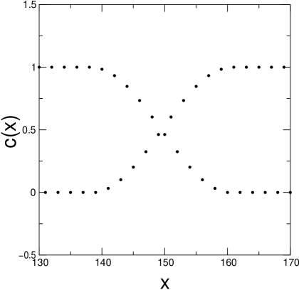
Figure 2: A typical ”soliton” of length $L=20$, an outcome of forward Euler integration of Eq. (13) on 1024 lattice points with periodic boundary conditions and random initial conditions at $\gamma=0.505$ (just above the bifurcation). There is a perfect agreement with the theoretical prediction, Eq. (III), up to the accuracy of the numerics (here, 4-5 significant digits)

The function $\beta_{k},\ k\in[0,\pi/l_{0}]$, is discrete for finite systems and becomes continuous at the thermodynamic limit. If $\beta_{k}$ never crosses zero there is no bifurcation and the homogenous solution $c_{n}=1/\beta_{0}$ is stable. The results for few types of interaction ranges, with the critical value $\gamma_{1}^{c}$ (where the instability occurs), and $k_{c}$ (the first excited mode), are summarized in Table I.

type	$\gamma_{r}$	$\beta_{k}$	$\rm{Instability\ condition}$
exponential	$(\gamma_{1})^{r/\xi}$	$\frac{sinh(|ln(\gamma_{1})|/\xi)}{cosh(|ln(\gamma_{1})|/\xi)-\cos(kl_{0})}$	$\rm{no\ instability}$
quadratic	$\frac{\gamma_{1}}{r^{2}}$	$1+2\gamma_{1}[\frac{\pi^{2}}{6}-\frac{\pi kl_{0}}{2}+\frac{(kl_{0})^{2}}{4}]$	$\gamma_{1}^{c}=\frac{6}{\pi^{2}}$, $k_{c}=\pi/l_{0}$
step	$\gamma_{r}=\{\begin{array}[]{cc}1&r\leq p\\ 0&r>p\\ \end{array}$	$\frac{sin(\frac{ka}{2}(2p+1))}{sin(\frac{ka}{2})}$	at large p $k_{c}=\frac{4pa}{3}$
gaussian	$(\gamma_{1})^{(r^{2}/\sigma^{2})}$	if $\sqrt{\sigma}>>l_{0}$ , $\sim\frac{\sigma}{2}\sqrt{\frac{\pi}{|ln(\gamma_{1})|}}exp\left(\frac{(\sigma kl_{0})^{2}}{4\sqrt{|ln(\gamma_{1})|}}\right)$	$\rm{no\ instability}$

Table 1: The function $\beta_{k}$ and the instability conditions for various types of nonlocal interactions. The results for the Gaussian case are in the continuum approximation.

It is interesting to note that these expressions may be generalized to yield a full, period doubling type, instability cascade. The m-th instability involves $2^{m}$ modes, and the steady state is $1/\sum_{k}\beta_{k}$, where the sum runs over all the ”active” modes. The condition for the $m+1$ bifurcation [activation of another $2^{m+1}$ modes] is the existence of a wavenumber $q$ such that $\sum_{k}\beta_{q-k}<0$, with the sum runs, again, over all $2^{m}$ active k-s. There are, however, some obstacles for the implication of these solutions above the first bifurcation. Degeneracies in $\beta_{k}$ (e.g., for $\gamma_{r}=\delta_{r,4}$, both $kl_{0}=\pi/4$ and $kl_{0}=3\pi/4$ are minima), and solitons between different stable phases (described below) may blur the native state. In this letter, though, $\beta_{k}$ is used only for the first, pattern-forming, instability criteria, and the details of the emerged structure are presented just for nearest-neighbor interaction.

Once diffusion is added to the system, its features changes, but not so much. The homogenous state is still characterized by $c_{n}=1/\beta_{0}$ and the first pattern formation instability appears when some $k$ mode satisfy:

$$\beta_{k}<-2\beta_{0}D[1-cos(kl_{0})].$$ (10)

Above this instability, the amplitudes of the modes are not equal,

$$A_{0}=\frac{\alpha_{k}}{\beta_{0}+\beta_{k}}\qquad A_{k}=\sqrt{\frac{\alpha_{k}(\beta_{0}+\beta_{k})-\beta_{0}}{\beta_{k}(\beta_{0}+\beta_{k})^{2}}}$$ (11)

and there are no zeroes of $c_{n}$. This result fits perfectly with the numerical data presented in figure (1). Again the m-th instability involves the activation of $2^{m}$ modes, Although the stability analysis is more complicated.

The question of pattern instability is thus translated to the determination of the minimal value of the Fourier coefficient of the weight function (or the ”weight series” $\gamma_{r}$). If the minimal value is smaller than some prescribed number (zero if there is no diffusion) instability takes place and patterns emerge. Unfortunately I am not familiar with a general theorem that sets bounds on the minimal value of the Fourier coefficient of a function based on its ”smoothness”, or other analytic properties, so any case should be considered separately, with the generic examples given in Table I.

III Domain wall structure

Above the pattern formation threshold generic initial conditions fail to yield perfect ”lattice”, as different domains reach saturation with different ”phases”. These domains are connected by soliton-like solutions of the time independent equation in the following sense: any stable solution (${\dot{c}}(x,t)=0$) should satisfy (in the continuum limit ),

$$D\frac{d^{2}c(x)}{dx^{2}}=c(x)-c(x)\int f(x-y)c(y)dy,$$ (12)

thus it looks like a trajectory of mechanical particle (with mass D) in a nonlocal potential, with $x$ as the ”time”. A domain wall is a finite size structure, so it must connect fixed points of this fictitious dynamics, i.e., a domain wall corresponds to heteroclinic orbit. In this section we consider these ”solitons” and look for their shape and size at different conditions. In order to simplify the discussion, only the nearest neighbor case is considered, both with and without diffusion.

With no diffusion and n.n. competition, (9) takes the form:

$$\frac{\partial c_{n}}{\partial\tau}=c_{n}\left[1-c_{n}-\gamma(c_{n+1}+c_{n-1})\right].$$ (13)

The uniform solution, in this case, is $c=\frac{1}{1+2\gamma}$, and the nonuniform solution is, either $c_{n}=1$ for odd n and $c_{n}=0$ for even, or vice versa. Stability analysis shows that the uniform solution becomes unstable at $\gamma_{c}=1/2$, and the zero-one phase is stable above this value. One may expect, though, to see a jump from homogenous to patterned (zero-one) phase at $\gamma_{c}$. However, if the initial conditions are taken from random distribution, there is a chance for a domain wall between two regions, as indicated by the numerical results presented in Figure (2).

Clearly, such a soliton should be a solution of the ”map”

$$c_{n+1}=\frac{1-c_{n}}{\gamma}-c_{n-1}.$$ (14)

of course, 01010101… (odd 0-s) and 101010101… (even 0-s) are already solutions of this equation. We are looking for the solution that connect these two fixed points. Such a trajectory begins in, say, 010101010 state, but then after the zero it gives not 1 but $x_{1}$. The dynamics now continue in a different trajectory, but $x_{1}$ should be selected such that after L steps of the map (for domain wall of size L) the 101010 solution is rendered. In a matrix form, the condition that determined $x^{L}_{1}$ ($x_{1}$ for a given L) is:

$$\left(\begin{array}[]{c}0\\ x^{L}_{1}\\ 1\end{array}\right)=\left[\begin{array}[]{ccc}-\frac{1}{\gamma}&-1&\frac{1}{\gamma}\\ 1&0&0\\ 0&0&1\end{array}\right]^{L}\left(\begin{array}[]{c}x^{L}_{1}\\ 0\\ 1\end{array}\right)=\mathcal{M}^{L}\left(\begin{array}[]{c}x^{L}_{1}\\ 0\\ 1\end{array}\right).$$ (15)

Where we assume symmetry of the soliton, so L must be even. In other words, the condition that determine $x^{L}_{1}$ is:

$$\left(\left[\begin{array}[]{ccc}-\frac{1}{\gamma}&-1&\frac{1}{\gamma}\\ 1&0&0\\ 0&0&1\end{array}\right]^{L}-\left[\begin{array}[]{ccc}0&1&0\\ 1&0&0\\ 0&0&1\end{array}\right]\right)\left(\begin{array}[]{c}x^{L}_{1}\\ 0\\ 1\end{array}\right)=0$$ (16)

Diagonalization of $\mathcal{M}$ is given by the matrix $\mathcal{S}$:

$$\mathcal{S}^{-1}\mathcal{M}\mathcal{S}=\mathcal{D}$$ (17)

where

$$\mathcal{D}=\left[\begin{array}[]{ccc}1&0&0\\ 0&-e^{-i\theta}&0\\ 0&0&-e^{-i\theta}\end{array}\right]$$ (18)

and $\theta=\arctan(\sqrt{4\gamma^{2}-1})=\arccos(\frac{1}{2\gamma})$.

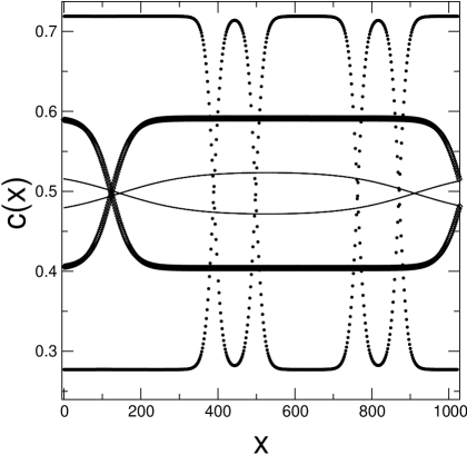
Figure 3: Solitons for nn interaction with $\gamma=0.505$ and $D=0.001$ (circles) $D=0.0012$ (heavy line) and $D=0.00124$ (line). $D_{c}=0.00124378$

The eigenvalue problem (16) may be written in terms of the diagonal matrix,

$$x^{L}_{1}=S_{11}-S_{12}\frac{r_{13}}{r_{23}}\frac{\cos(\frac{L\theta}{2}+\varphi)}{\cos(\frac{L\theta}{2}+\eta)}$$ (19)

and using $S_{12}=S_{13}^{*}=r_{12}e^{i\varphi}$ and $S_{22}=S_{23}^{*}=r_{23}e^{i\eta}$ it implies that,

$$x^{L}_{1}=\frac{1}{2\gamma+1}\left[1+\sqrt{\frac{1-T_{L-1}(1/2\gamma)}{1-T_{L+1}(1/2\gamma)}}\right]$$ (20)

where $T_{n}(x)$ is the n-th Chebyshev polynomial of the first kind. After determining $x^{L}_{1}$ the same method may be used to derive a general expression for all the elements of the size L soliton ($x^{L}_{m}$, where $1\leq m\leq L$):

$$x^{L}_{m}=\frac{1}{2\gamma+1}\left[1+(-1)^{m}\sqrt{\frac{2\gamma[1-T_{2m-1}(1/2\gamma)]}{2\gamma-1}}\right.$$

$$\left.-(-1)^{m}\frac{2\gamma x^{L}_{1}}{8\gamma^{2}-2}\sqrt{1+T_{2m}(1/2\gamma)}\right]$$ (21)

and it fits perfectly the numerical experiment presented in Fig. (2, see captions).

The above analysis gives the shape of a soliton for any prescribed length $L$,but simulation indicates that only one soliton size $L$ is selected for any set of parameters, and its length diverges as $\gamma$ approaches its critical value. Looking carefully at the solutions (III) one realizes that all other possible solitons admit values for some of the $x_{m}$-s that are either negative or larger than one, so these options are unphysical (negative) or unstable to small perturbations.

The actual $L(\gamma)$ may be forecasted by a rough argument based on a continuum approach. Defining the local deviation from the one-zero solution, $c_{n}=1$ and $c_{n\pm 1}=0$,

$$c_{n\pm 1}=\delta_{n\pm 1}\qquad\qquad c_{n}=1-\delta_{n}$$ (22)

and plugging it into Eq. (14) gives,

$$\delta_{n+1}+\delta_{n-1}=\frac{\delta_{n}}{\gamma}.$$ (23)

Subtracting of $2\delta_{n}$ from both sides and taking the continuum limit (i.e., assuming that the changes in $\delta$ from site to site are small compared to $l_{0}$, here taken to be unity) one gets,

$$\nabla^{2}\delta(x)=-\frac{4\epsilon}{1+2\epsilon}\delta(x)$$ (24)

with $\epsilon\equiv\gamma-\gamma_{c}$ goes to zero at the transition, so $1+2\epsilon\approx 1$. The solution of Eq. (24) that satisfies the boundary conditions $\delta(0)=0$ together with $\delta(L)=1$ is

$$\delta(x)=\frac{sin(2\sqrt{\epsilon}x)}{sin(2\sqrt{\epsilon})L}.$$ (25)

This expression fails to converge smoothly to the ”background” ordered 010101 phase (at x=0 it has a finite slope), and is also asymmetric. Put it another way, there are no nontrivial heteroclinic orbits for a parabolic potential. On the other hand, close to the transition, where the size of the domain wall is large, it seems that it should fit a solution of the continuum approximation. The only way out is to pick a soliton size L such that the continuum equation admit no solution at all, i.e.,

$$L=\frac{\pi}{2\sqrt{\epsilon}}.$$ (26)

Such a choice forces us back to the discrete equation (14) and its solution (III). This argument turns out to give the right length of the stable soliton in the large $L$ ($\epsilon\to 0$) limit, as shown in Fig. (4).

Let us consider now the domain walls for the finite diffusion case. As seen in Fig. (3), there are also solitons for the finite diffusion case, but now they admit tails that asymptotically looks like $\delta\sim exp(-x/\xi)$, and $\xi$ diverges at the transition [e.g., at $D_{c}=\frac{2\gamma-1}{4(2\gamma+1)}$ for nearest neighbor interaction]. Defining a vectorial ”order parameter” according to the larger $c$ values, soliton solution interpolates between $(1,0)$ (larger $c$ on the odd sites) to $(0,1)$ (even sites), and its shape is given by the saddle point solution of the appropriate dynamics. Although the determination of its full shape is difficult, it is possible to determine $\xi$ by linearizing around one fixed point. For small deviations, $c_{n}=A_{0}+A_{\pi/l_{0}}-\delta_{n}$ and $c_{n\pm 1}=A_{0}-A_{\pi/l_{0}}+\delta_{n\pm 1}$ and Eq. (14) yields the two coupled linear equations for odd and even n-s:

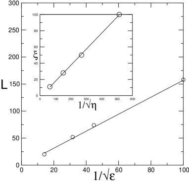
Figure 4: Soliton size ($L$) as a function of $1/\sqrt{\epsilon}$, ($\epsilon=\gamma-\gamma_{c}$), for a nearest-neighbor interaction without diffusion. The circles are the results of a numerical simulation and the line is $\pi/(2\sqrt{\epsilon})$. In the inset, the characteristic length of the soliton tail, $\xi$, is plotted against $1/\sqrt{\eta}$ for $\gamma=0.505$ for the solitons shown in Fig. (3). The circles come from the numerics and the line is the best linear fit that give a slope of 0.198, to be compared with $1/\sqrt{32}=0.177$.

$$(2s+2d\gamma-1+2D)\delta_{n}^{even}+(D-\gamma s)(\delta_{n+1}^{odd}+\delta_{n-1}^{odd})=0$$ (27)

$$(2d+2s\gamma-1+2D)\delta_{n}^{odd}+(D-\gamma d)(\delta_{n+1}^{even}+\delta_{n-1}^{even})=0.$$

where $s\equiv A_{0}+A_{\pi/l_{0}}$ and $d\equiv A_{0}-A_{\pi/l_{0}}$. These coupled equation may be solved with the ansatz $\delta^{even}\sim a_{1}\exp(-x/\xi),\ \ \delta^{odd}\sim a_{2}\exp(-x/\xi)$ to give,

$$\xi=\left[arccosh\left(\frac{1}{2}\sqrt{\frac{(4+64D^{2}-32D)\gamma^{2}+(20D-8D^{2}-4)\gamma+1-20D^{2}}{D(\gamma-D-2\gamma D)}}.\right)\right]^{-1},$$ (28)

As the diffusion constant approaches its critical value, $D=D_{c}-\eta$, $\xi$ diverges like $1/\sqrt{32\eta}$. This prediction is tested in the caption of Fig. (4) against the numerics and there is reasonable quantitative agreement, given the difficulties in getting reliable numerical accuracy for the slope of the logarithmic tail of the soliton.

IV concluding remarks

The model of logistic growth with long range interaction term may serve as a generic, minimal model for competition for common resource and pattern formation in excited media. In this paper this model has been analytically discussed, with two main outcomes. First, a general scheme for the identification of the pattern forming instability has been presented, along with explicit results for few common cases. Second, the defected solutions for random initial conditions has been presented and analyzed, and their characteristic length that diverges at the transition is calculated.

The patterned solutions (like the 010101 for n.n. interactions) are stable against small perturbation (like a low amplitude white noise). If instead of …01010101.. one have …01010(0.9)01.. the 0.9 site relaxes to 1. The domain walls, on the other hand, are much less stable, and their density and dynamics has to be strongly effected by an external noise. This is very much like the situation in magnetic system, where the response functions of the material are basically determined by the domain walls and not by the ”bulk”. In magnetic systems, however, one may define the state of the system at finite temperature ad a minimum of the free energy function and consider the effect of noise simply as temperature increase. The situation seems to be different for the long range competition model: no simple Liapunov function exist for this system, and the steady state is not derived from some variational principle. In spite of that it is plausible to assume that the defected solutions determine the response function of the segregated phase, and maybe an effective dynamical equations for the solitons may be set up to give an approximate Liapunov function for this system.

V Acknowledgements

I thank Prof. David Kessler for helpful discussions and comments.

References

- (1) R. A. Fisher, Ann. Eugenics 7, 353, (1937).
- (2) A. Kolomogoroff, I. Petrovsky and N. Piscounoff, Moscow Univ. Bull. Math. 1,1 (1937).
- (3) W. van Saarloos, Physics Reports 386, 29,(2003).
- (4) See, e.g. J.D. Murray, Mathematical Biology (Springer-Verlag, New-York, 1993), and D. Walgraef, Spatio-temporal pattern formation (Springer-Verlag, New-York 1996).
- (5) J.B. Wilson and A.D.Q. Agnew, Adv. Ecol. Res. 23, 263 (1992); R. Lefever and O. Lejeune, Bull. Math. Biol. 59, 263 (1997); J. von Hardenberg, E. Meron, M. Shachak and Y. Zarmi, Phys. Rev. Lett. 87 198101 (2001).
- (6) N.M. Shnerb, P. Sarah, H. Lavee and S. Solomon, Phys. Rev. Lett. 90, 038101 (2003).
- (7) E. Ben-Jacob, I. Cohen and H. Levine, Adv. in Phys. 49, 395 (2000).
- (8) H. Sayama, M.A.M. de Aguiar, Y. Bar-Yam and M. Baranger, Phys. Rev. E 65, 051919 (2002).
- (9) M. A. Fuentes, M. N. Kuperman and V.M. Kenkre, Phys. Rev. Lett. 91, 158104 (2003).
- (10) D.R. Nelson and N.M. Shnerb, Phys. Rev. E 58, 1383 (1998), Appendix B.