A density-functional approach to fermionization in the 1D Bose gas

Abstract

A time-dependent Kohn-Sham scheme for 1D bosons with contact interaction is derived based on a model of spinor fermions. This model is specifically designed for the study of the strong interaction regime close to the Tonks gas. It allows us to treat the transition from the strongly-interacting Tonks-Girardeau to the weakly-interacting quasicondensate regime and provides an intuitive picture of the extent of fermionization in the system. An adiabatic local-density approximation is devised for the study of time-dependent processes. This scheme is shown to yield not only accurate ground-state properties but also overall features of the elementary excitation spectrum, which is described exactly in the Tonks-gas limit.

1 Introduction

Density-functional theory (DFT) provides a unique framework for the treatment of quantum many-body systems beyond the realm of perturbation theory. While ground-state DFT, based on the theorems of Hohenberg, Kohn, and Sham [1, 2] deals with the energy and the density profile of inhomogeneous ground states, the time-dependent generalization of these theorems by Runge and Gross [3] in principle allows the study of time-dependent processes and excited states. Further development of the time-dependent DFT has shown that it is advantageous to consider functionals simultaneously of the density and the current [4] in order to go beyond the simplistic adiabatic approximation and the microscopic Navier-Stokes equations for the electron fluid have been derived elegantly this way [5].

In this paper we will apply DFT to the study of fermionization in the system of 1D bosons with contact interaction. In the case of infinite interaction strength, the model is also known as the Tonks-Girardeau gas [6] and maps exactly to the system of non-interacting spinless fermions with identical energy spectrum and single-particle density. In fact, it has been shown by Cheon and Shigehara [7] that the exact mapping between the original Bose system and a Fermi system can be extended to arbitrary interaction strength at the expense of a highly singular interaction in the fermionic picture. For the homogeneous Bose gas, exact solutions for stationary states at arbitrary interaction strength can be found using the Bethe ansatz [8, 9, 10]. Although the exact solutions show a continuous transition between the perturbative regime of weakly-interacting bosons and the strongly correlated, fermionized regime, they do not prove very useful for the study of time-dependent processes or inhomogeneous situations. Neither do they provide us with a simple, intuitive picture of how strong the degree of fermionization is in a given system. The crossover from the quasicondensate to the fermionized Tonks gas has also been studied in Refs. [11, 12]

Inspired by the works of Haldane [13], Sutherland [14], and others on the concept of exclusion statistics describing a crossover between fermionic and bosonic statistics in 1D systems, we study a model which explicitely allows this transition and provides an intuitive picture of the degree of fermionization. In order to devise a practical scheme for treating time-dependent and inhomogeneous systems we employ DFT and develop a time-dependent Kohn-Sham formalism based on the auxiliary model system of $N$ non-interacting spin-$(\nu-1)/2$ fermions. This model is chosen because the spin degeneracy may simulate the level attraction or the bunching of single-particle quasi momenta in the interacting bosonic system [8]. The interaction energy of the Bose system is simulated by the kinetic energy of the spin-degenerate fermions. In this work we will study the model in the simplest and most generic approximation: the adiabatic local density approximation (ALDA). The limiting case of infinite interaction strength is obtained easily and is treated exactly with $\nu=1$. The opposite limit of weak interaction can also be treated accurately within the proposed formalism with $\nu=N$ where the perturbative Gross-Pitaevskii and Bogoliubov equations are recovered asymptotically. In the general case of arbitrary interaction strength, the spin degeneracy $\nu$ is fixed by requiring the correct low-energy asymptotics of the excitation spectrum, which is analyzed in the framework of linear-response theory. The resulting model is suited for the study of time-dependent processes in inhomogeneous 1D Bose gases close to the Tonks-gas limit. The properties of this approximate model are analyzed and systematic improvements are suggested.

Before developing the general theory we want to point out that DFT is not commonly used to discuss the theory of ultra-cold bosonic gases although many standard approximations can be derived in this framework. Only few papers therefore explicitely suggested to apply DFT in this context, see e.g. Refs. [15, 16, 17, 18, 19, 20, 21], where the time-dependent DFT of superfluids [20, 21] is particularly far developed. The case of strongly interacting bosons in 1D has been considered by Kolomeisky et al. [17] who suggested a generalization of the Gross-Pitaevskii equation of the following form:

$$i\hbar\frac{\partial}{\partial t}\psi(x,t)=\left\{-\frac{\hbar^{2}}{2m}\frac{\partial^{2}}{\partial x^{2}}+v_{\mathrm{ext}}(x,t)+\phi(n(x,t))\right\}\psi(x,t)$$ (1)

Here, $\psi(x,t)$ is a time-dependent complex field and $n(x,t)=|\psi(x,t)|^{2}$ is the one-dimensional density. The function $\phi(n)$ provides the nonlinear term. Kolomeisky et al. suggested to use the chemical potential of the Tonks-Girardeau gas

$$\phi(n)=\phi^{{\mathrm{(}TG)}}(n)\equiv\frac{\pi^{2}\hbar^{2}}{2m}n^{2}$$ (2)

whereas the Gross-Pitaevskii equation is recovered for

$$\phi(n)=\phi^{{\mathrm{(}GP)}}(n)\equiv g_{{\mathrm{1}D}}n.$$ (3)

We will refer to Eq. (1) as the bosonic LDA because this equation may be derived as a Kohn-Sham equation in the ALDA using a Bose condensate as the auxiliary non-interacting system for the Tonks gas and the weakly interacting Bose gas, respectively. The same equation also applies for 1D bosons with arbitrary interaction strengths and was used by Öhberg and Santos [18]. In this case, $\phi(n)$ represents the exactly known chemical potential of the Lieb-Liniger model (at $T=0$). The bosonic LDA equation (1) is almost identical to a set of hydrodynamic equations[22, 23] derived from general hydrodynamic arguments assuming local equilibrium, the only difference being a kinetic energy pressure term (see e.g. [24]).

It may be questioned whether the choice of a Bose condensate as the auxiliary non-interacting system of the Kohn-Sham formalism is the ideal starting point for treating a strongly interacting Bose gas in 1D which is not condensed[25, 6]. Indeed it has been shown in the Tonks-Girardeau limit of impenetrable point bosons, that phase coherence is grossly overestimated by Eq. (1) leading to wrong predictions for interference properties [26, 27]. Phase and density are conjugate variables in a quantum field theory and may coexist in the weakly-interacting Bose condensate, which is close to a classical field. It is known already in the perturbative regime, that phase fluctuations are very important in 1D [28, 12]. In the ultimate limit of the Tonks-Girardeau gas, the concept of phase looses its meaning and the governing equations should be rather based on the density alone. For this reason the hydrodynamic approximations employed in Refs. [22, 23], where the concept of a phase does not appear, are on a safer footing than the bosonic LDA equation of Kolomeisky where phase-coherence is built into the theory.

Moreover, the excitation spectrum and density of the the Tonks-Girardeau gas is identical to the corresponding properties of a gas of independent spinless fermions due to the Bose-Fermi mapping. Already in his original paper[8], Lieb pointed out, that the fermionic character of the excitation spectrum prevails at finite interaction strength and introduced two elementary branches of excitations which he called type I and type II. Type I excitations result from exciting a particle from the edge of the 1D Fermi sphere to an unoccupied orbital. Thus type I excitations are the particle-hole excitations of the highest possible energy for a given momentum. Type II excitations, on the contrary, are the excitations of the lowest possible energy for a given momentum. They can be seen as taking a particle from the inside of the Fermi sphere and putting it to the first free orbital on the outside.

Only type I excitations are found by standard bosonic methods like Bogoliubov perturbation theory or linear response in Eq. (1) whereas type II excitations and the fermionic character of the spectrum remain hidden. We want to mention at this point that a possible connection between type II excitations and dark solitons in variations of Eq. (1) has been pointed out in the literature [29, 17, 30, 31].

2 An exotic Kohn-Sham scheme

2.1 Variational principles

The basic scheme of DFT is the Hohenberg-Kohn variational principle. It allows the ground-state energy $E_{0}$ and one-particle density $n(x)$ of a given many-particle system to be found by variationally minimizing the energy functional

$$E_{v}[n]=F_{\mathrm{HK}}[n]+\int v_{\mathrm{ext}}(x)n(x)dx.$$ (4)

Here $v_{\mathrm{ext}}(x)$ is the external potential and the Hohenberg-Kohn functional $F_{\mathrm{HK}}[n]$ is universal in that it does not depend on the external potential. The scheme of Kohn and Sham proceeds by partitioning the unknown functional $F_{\mathrm{HK}}[n]$ as

$$F_{\mathrm{HK}}[n]\equiv T_{s}[n]+E_{\mathrm{KS}}[n],$$ (5)

where $T_{s}[n]$ is the kinetic energy of a ficticious, auxiliary system of particles interacting only with a single-particle potential $v_{s}$, which has the same density $n(x)$ as the original system. The external potential $v_{\mathrm{ext}}$ is contained in $v_{s}=v_{\mathrm{ext}}+v_{\mathrm{KS}}$ where $v_{\mathrm{KS}}[n]=\delta E_{\mathrm{KS}}/\delta n$ is a universal functional of the density depending only on the structure and internal interactions of the original and auxiliary many-body problem but not on the external potential. Once an (approximate) expression for $v_{\mathrm{KS}}[n]$ has been found, the density of the system in a given external potential $v_{\mathrm{ext}}$ is easily found by solving the Kohn-Sham equations, a set of nonlinear independent-particle equations. Kohn and Sham in their original publication[2] used the auxiliary system of noninteracting spin-1/2 fermions while interested in systems of interacting electrons. However, it has been pointed out that the choice of the auxiliary system is somewhat arbitrary and rather a matter of convenience than dictated by laws of nature [32].

2.2 Hamiltonian

We start with the usual Hamiltonian for $N$ bosons in 1D with point interactions of Ref. [8], augmented with a possibly time-dependent external potential $v_{\mathrm{ext}}(x,t)$:

$$H=\sum_{i=1}^{N}\left\{-\frac{\hbar^{2}}{2m}\frac{\partial}{\partial x_{i}}+v_{\mathrm{ext}}(x_{i},t)\right\}+2g_{\mathrm{1D}}\sum_{i<j}\delta(x_{i}-x_{j}),$$ (6)

where $g_{\mathrm{1D}}=2\hbar^{2}/(m|a_{\mathrm{1D}}|)$ is the interaction parameter and $a_{\mathrm{1D}}$ is the one-dimensional scattering length[11].

The exact many-body eigenstates and the complete excitation spectrum of the Hamiltonian (6) in the homogeneous system where $v_{\mathrm{ext}}=0$ with periodic boundary conditions have been found by Lieb and Liniger using the Bethe ansatz [8, 9]. The ground state energy is

$$E_{0}^{\mathrm{hom}}=N\frac{\hbar^{2}n^{2}}{2m}e(\gamma)$$ (7)

where $e(\gamma)$ is the dimensionless energy per particle in the Lieb-Liniger model and $\gamma=2/(n|a_{\mathrm{1D}}|)$ is the single dimensionless parameter of the homogeneous gas with the one-dimensional single-particle density $n=N/L$ of $N$ particles in a box of length $L$. The function $e(\gamma)$ is defined as the solution of a Fredholm equation and can be obtained numerically to any desired accuracy. The chemical potential of the homogeneous Lieb-Liniger gas at density $n$ is given by

$$\mu_{\mathrm{LL}}(n)=\frac{d}{dN}E_{0}^{\mathrm{hom}}=\frac{2\hbar^{2}}{m|a_{\mathrm{1D}}|^{2}}f(\gamma),$$ (8)

where $f(\gamma)=[3e(\gamma)-e^{\prime}(\gamma)]/\gamma^{2}$ is a dimensionless function. The asymptotic behaviour of $e(\gamma)$ and $f(\gamma)$ is known for large and small $\gamma$ [8] and, furthermore, the functions are tabulated for intermediate values of $\gamma$ in Ref. [22] .

2.3 Functionals and Kohn-Sham equations

Consider a physical system of $N$ noninteracting and indistinguishable fermions with spin $(\nu-1)/2$. For simplicity let us consider the case where $\nu$ divides $N$ and assume that all orbitals are nondegenerate. In the ground state $\tilde{N}$ orbitals will be occupied with $\nu$ particles each when $\nu\tilde{N}=N$. The kinetic energy is

$$T_{s}[n]=-\frac{\hbar^{2}}{2m}\nu\sum_{i=1}^{\tilde{N}}\int\varphi_{i}^{*}(x)\frac{\partial^{2}}{\partial x^{2}}\varphi_{i}(x)\;dx.$$

The Kohn-Sham equations are found by functional differentiation with respect to $\varphi_{i}^{*}(x)$:

$$\varepsilon_{i}\varphi_{i}(x)=\left\{-\frac{\hbar^{2}}{2m}\frac{\partial^{2}}{\partial x^{2}}+v_{\mathrm{ext}}(x)+v_{\mathrm{KS}}[n](x)\right\}\varphi_{i}(x).$$ (9)

The potential $v_{\mathrm{KS}}[n]=\frac{\partial E_{\mathrm{KS}}[n]}{\partial n}$ is the mean-field potential of Kohn-Sham theory and represents the unknown rest of the functional. In regular electronic DFT, $v_{\mathrm{KS}}[n]$ would be written as a sum of the Hartree potential and the exchange-correlation potential. The density is found self-consistently by summing over all occupied ($\in$) orbitals

$$n(x,t)=\nu\sum_{i\in}|\varphi_{i}(x,t)|^{2}$$

The ground state density $n(x)$ is obviously time-independent and only the $\tilde{N}$ levels with the lowest energies $\varepsilon_{i}$ will be occupied. The generalization to the corresponding time-dependent Kohn-Sham equations along the lines of the Runge-Gross theorems [3] is obvious:

$$i\hbar\partial_{t}\varphi_{i}(x,t)=\left\{-\frac{\hbar^{2}}{2m}\frac{\partial^{2}}{\partial x^{2}}+v_{\mathrm{ext}}(x,t)+v_{\mathrm{KS}}[n](x,t)\right\}\varphi_{i}(x,t).$$ (10)

We note that Eq. (10) is still exact. We now proceed in approximating $v_{\mathrm{KS}}[n]$ in a local-density approximation.

To this end, the remaining unknown term $E_{\mathrm{KS}}[n]$ is approximated by $E_{\mathrm{KS}}[n]\approx E_{\mathrm{KS}}^{\mathrm{LDA}}(n)=E_{0}^{\mathrm{hom}}-T_{s}^{\mathrm{hom}}$, where $T_{s}^{\mathrm{hom}}$ is the noninteracting kinetic energy of the homogeneous gas. It is simply found by summing the contributions from the $\tilde{N}$ orbitals in the Fermi sphere and multiplying with the degeneracy $\nu$:

$$T_{s}^{\mathrm{hom}} = \nu\frac{\hbar^{2}}{2m}\sum_{k=-(\tilde{N}-1)/2}^{(\tilde{N}-1)/2}\left(\frac{2\pi k}{L}\right)^{2}$$ (11)

$$= N\frac{\hbar^{2}\pi^{2}{n}^{2}}{6m\nu^{2}}\left(1-\frac{1}{\tilde{N}^{2}}\right)$$

where $L$ is the length of a box with periodic boundary conditions, $n={N}/L=n$ is the line density and $\tilde{N}$ has been assumed odd.

Before taking the derivative $\frac{\partial F_{\mathrm{HK}}[n]}{\partial n}$ in order to find an expression for $v_{\mathrm{KS}}$ we have to consider what to do with the term $1/\tilde{N}$. If $\tilde{N}=1$ the contribution from the kinetic energy vanishes and we arrive at the bosonic LDA of Eq. (1). However, if $\tilde{N}$ is of the order of $N$, we may disregard the term $1/\tilde{N}$ in the limit of large $N$. In fact it is not consistent to keep this term if we approximate the Lieb-Liniger energy with the bulk value as this is only valid in the limit $N\to\infty$. In the following we will therfore drop this term and arrive at

$$v_{\mathrm{KS}}^{\mathrm{LDA}}(x,t) = \frac{d}{dN}\left(E_{0}^{\mathrm{hom}}-E_{\mathrm{kin}}\right)|_{n=n(x,t)}$$ (12)

$$= \mu_{\mathrm{LL}}(n)-\frac{\hbar^{2}\pi^{2}n^{2}}{2m\nu^{2}},$$

where the chemical potential $\mu_{\mathrm{LL}}(n)$ of the homogeneous (Lieb-Liniger) gas at density $n$ is given by Eq. (8). The remaining parameter $\nu$ will be determined by a consistency condition on the excitation spectrum that will be derived in the following paragraph.

2.4 Excitation spectrum from linear-response theory

Lieb pointed out that the excitation spectrum of the 1D Bose gas resembles that of the 1D Fermi gas and likewise has a particle-hole type of structure — at any value of the interaction strength [9]! The spectrum of the homogeneous gas may be equally well described by two branches of elementary excitations $\epsilon^{{\mathrm{I}}}(k)$ and $\epsilon^{{\mathrm{II}}}(k)$. Both branches have the same slope for $k\to 0$ and therefore lead to the same speed of sound $v_{s}=d\epsilon^{{\mathrm{I}}}/dk|_{k=0}=d\epsilon^{{\mathrm{II}}}/dk|_{k=0}$. Bogoliubov perturbation theory yields an approximation only for the branch $\epsilon^{{\mathrm{I}}}(k)$. In the time-dependent Kohn-Sham model introduced above, a particle-hole type excitation spectrum arises naturally. The elementary excitations may be found by solving for the resonant frequencies of the time-dependent equation (10) in the linear-response limit. The resulting excitation energies are given by differences of the orbital energies of the stationary Kohn-Sham orbitals modified by interaction contributions from the nonlinear mean-field $v_{\mathrm{KS}}^{\mathrm{LDA}}$.

The derivation of the linear response equations is the same as for the LDA in the much studied electronic systems and very similar to the time-dependent Hartree-Fock or random-phase approximation (see e.g. [33]) and is summarized in the appendix. Here we want to note that the linear response correction to the spectrum of the Kohn-Sham system is proportional to the derivative $dv_{\mathrm{KS}}/dn$. From the explicit linear response equations for the homogeneous system it can be seen that type I and type II excitations have a different slope at $k=0$, except for the situation where

$$v_{\mathrm{KS}}^{\prime}(n)=0.$$ (13)

This argument is detailed in the Appendix where the linear response equations in the small momentum limit are solved exactly. Using the expression (12) for $v_{\mathrm{KS}}$ we easily find the correct value for the number of modes in the fermionic Kohn-Sham equations (10):

$$\tilde{N}=N\sqrt{-\frac{\gamma^{3}}{2\pi^{2}}f^{\prime}(\gamma)}.$$ (14)

The value of $\tilde{N}/N\equiv 1/\nu$ is a measure of the degree of fermionization in the system. When $\tilde{N}/N=1$ the system is completely fermionized whereas $\tilde{N}/N\to 0$ indicates a purely bosonic system with a Bose condensate as the ground state. The functional dependence of $\tilde{N}/N$ on the interaction strength $\gamma$ is shown in Figure 1.

Qualitatively the picture agrees with the results of Girardeau and Wright [34] who modelled the BEC-Tonks crossover by a mixture of a pair-correlated Bose liquid with a non-interacting Fermi gas in a variational framework. We would like to point out, that $\tilde{N}$ is a global parameter whereas $\gamma$ is local and varies in an inhomogeneous system. Therefore the condition (14) should be used with care and we expect the present model to be most useful for nearly homogeneous systems.

Although it would be desirable to find an approximation for the condensate fraction from our model, it should be noted that Kohn-Sham DFT as used here generally does not model the many-body wavefunction but gives direct access only to energies and the diagonal part of the single-particle density matrix. The information about off-diagonal long range order and condensate fraction, however, is contained in the inaccessible off-diagonal part of the single-particle density matrix. Nevertheless it should be pointed out that the fractional occupation of the Kohn-Sham orbitals $\tilde{N}^{-1}$ in our model, which is reminiscent of a condensate fraction, vanishes in the thermodynamic limit where $N\to\infty$ at $\gamma=const.$ consistent with the general result that there is no Bose condensate in the $T=0$ homogeneous interacting Bose gas [35, 36].

An important question related to the condensate fraction is local phase coherence [26, 27]. From the construction of the Kohn-Sham model it appears difficult to define expectation values for the phase operator in this scheme. However, the time-dependent DFT does contain information about local phase coherence to the degree that is necessary to correctly describe the supression of interference patterns in the dynamics.

The approximation scheme defined by Eqs. (10), (12), and (14) is the main subject of this paper and shall be referred to as fermionic LDA. In the remainder of this paper we will analyze the predictions of this model and compare with the exact solutions of the Lieb-Liniger model and other approximations.

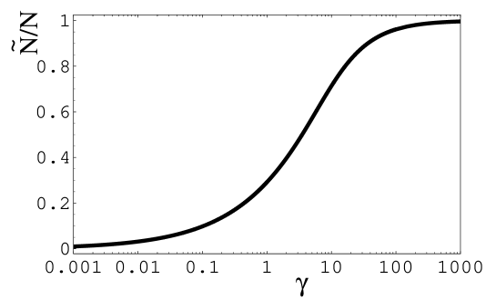
Figure 1: The parameter $\tilde{N}/N$ from Eq. (14) indicates the degree of fermionization in the system. Here it is plotted as a function of the dimensionless interaction strength of the Lieb-Liniger model $\gamma$.

3 Properties

3.1 Excitations of the homogeneous gas

It is interesting to calculate the dispersion for the elementary excitations of type I and II, which can be done analytically since the linear-response corrections vanish due to Eq. (13). In the homogeneous gas, the mean field $v_{\mathrm{KS}}$ is constant and the Kohn-Sham single-particle energies become

$$\epsilon_{p}=\frac{2\pi^{2}\hbar^{2}}{mL^{2}}p^{2}+v_{\mathrm{KS}},$$

where $p$ is any integer and $\hbar k_{p}=\hbar p\,2\pi/L$ is the momentum. In the ground state all orbitals with $p<F$ are occupied where $F=(\tilde{N}-1)/2$ is the index of the Fermi momentum $\hbar k_{F}$. The energies of particle-hole excitations of momentum $\hbar k_{q}$ are given by the difference

$$\epsilon_{p}-\epsilon_{p-q} = \frac{\hbar^{2}}{2m}n^{2}\frac{4\pi^{2}}{N^{2}}q(2p-q).$$ (15)

Figure 2 illustrates the discrete excitation spectrum obtained for a finite number of particles in a box with periodic boundary conditions. Type I and II excitations are the upper and lower bounds of the elementary excitation spectrum, respectively. The fermionic DFT is seen to slightly overestimate the energies of type I excitations and underestimate the energies of type II excitations at large momentum while the correct asymptotes are obtained for small momenta.

From Eq. (15) we can construct explicit expressions for type I and type II excitations. Type I excitations are defined by exciting a particle with the Fermi momentum $\hbar k_{F}$ into an unoccupied orbital with $p=F+q$ whereas type II excitations take a particle from inside the Fermi sphere to the lowest unoccupied orbital with $p=F+1$. In terms of the dimensionless momentum

$$\tilde{p}=\frac{\hbar k_{q}}{\hbar n}=\frac{2\pi q}{N}$$

of the excitations we obtain

$$\epsilon^{\mathrm{I}}(\tilde{p})=\frac{\hbar^{2}}{2m}n^{2}\tilde{p}\left[2\pi\left(\frac{1}{\nu}-\frac{1}{N}\right)+\tilde{p}\right].$$ (16)

Correspondingly we find for type II

$$\epsilon^{\mathrm{II}}(\tilde{p})=\frac{\hbar^{2}}{2m}n^{2}\tilde{p}\left[2\pi\left(\frac{1}{\nu}+\frac{1}{N}\right)-\tilde{p}\right].$$ (17)

Expressions for the elementary excitation spectrum of the interacting gas can be derived using equation (14). In the thermodynamic limit we obtain

$$\epsilon^{\mathrm{I}}(\tilde{p}) = \frac{\hbar^{2}}{2m}n^{2}\tilde{p}\left[\sqrt{-2\gamma^{3}f^{\prime}(\gamma)}+\tilde{p}\right],$$ (18)

$$\epsilon^{\mathrm{II}}(\tilde{p}) = \frac{\hbar^{2}}{2m}n^{2}\tilde{p}\left[\sqrt{-2\gamma^{3}f^{\prime}(\gamma)}-\tilde{p}\right].$$ (19)

These dispersion relations ought to be compared with the exact ones and with earlier approximations. First of all we note that both dispersions relations indeed lead to the same speed of sound

$$\left.\frac{d\epsilon^{\mathrm{I/II}}}{dp}\right|_{p=0}=c_{s}\equiv\frac{2\hbar}{m|a_{\mathrm{1D}}|}\sqrt{-\frac{\gamma}{2}f^{\prime}(\gamma)},$$ (20)

which is identical to the exact result of the Lieb-Liniger model[9].

The type II excitations, as discussed by Lieb, have the character of elementary excitations for $\tilde{p}\leq\pi$ and at this point the slope $d\epsilon^{\mathrm{II}}/d\tilde{p}$ vanishes. This condition is strictly fulfilled by Eq. (19) only in the Tonks-gas limit $\gamma\to\infty$ where the equations become exact. In the general case, $\epsilon^{\mathrm{II}}(\tilde{p})$ of Eq. (19) has a maximum at $\tilde{p}_{m}<\pi$ and $\tilde{p}_{m}$ approaches 0 as $\gamma\to 0$. This observation is related to the fact that the umklapp transition of taking one particle from one side of the Fermi-sphere to the other is not described correctly in the considered fermionic Kohn-Sham model. Therefore our approach is limited to describing type II excitations in the long-wavelength limit and works best for large $\gamma$.

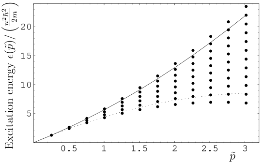
Figure 2: Shown are excitation energies of a homogeneous system with 25 particles at $\gamma=16.3$. Dots indicate the particle-hole excitation in the Kohn-Sham model with $\tilde{N}/N=0.8$ from Eq. (15). The full and dotted lines show the exact type I and II excitations for this finite system from the numerical solution of Yang’s equation [9, 37], respectively.

3.2 Comparison with bosonic LDA

The bosonic LDA of Eq. (1) is simply the single-mode case with $\tilde{N}=1$ of the general fermionic Kohn-Sham formalism in this paper. The linear-response equations (31) for this case coincide with the Bogoliubov-de Gennes equations derived in Refs. [18, 19]. It is instructive to derive explicit expressions for the excitations of a homogeneous gas, which appear not to be available in the literature. Eqs. (31) now become

$$(\epsilon_{q}-\epsilon_{0}+\frac{N\phi^{\prime}}{L})u_{q}+\frac{\nu\phi^{\prime}}{L}v_{q} = \hbar\omega u_{q}$$ (21)

$$(\epsilon_{q}-\epsilon_{0}+\frac{N\phi^{\prime}}{L})v_{q}+\frac{\nu\phi^{\prime}}{L}u_{q} = -\hbar\omega v_{q}$$ (22)

where $\phi^{\prime}=d\phi/dn$ and we have set $X_{hp}=u_{p-h}$ and $Y_{hp}=v_{h-p}$. With

$$\epsilon_{q}-\epsilon_{0}=\frac{2\pi^{2}\hbar^{2}q^{2}}{mL^{2}}$$

we find the simple solution

$$\hbar\omega=\pm\sqrt{\frac{\hbar^{2}k_{i}^{2}}{2m}(\frac{\hbar^{2}k_{i}^{2}}{2m}+2n\phi^{\prime})}.$$ (23)

Only the plus sign contributes here, the minus sign is a well understood artifact of linear response theory. In terms of the dimensionless momentum $\tilde{p}=k/n$ we find the following final result for the excitation spectrum of the bosonic LDA with $\phi(n)=\mu_{\mathrm{LL}}(n)$:

$$\hbar\omega=\frac{\hbar^{2}}{2m}n^{2}\sqrt{\tilde{p}^{2}(\tilde{p}^{2}-2\gamma^{3}f^{\prime}(\gamma))}.$$ (24)

In contrast to the excitation spectrum described by Lieb, there is only one excitation branch in the linear response of the bosonic LDA. Comparing with Eqs. (21) and (22) we see that the first terms in the expansions around $k=0$ and $k=\infty$ are identical but there are discrepancies in between. The speed of sound is again the exact result $c_{s}$ as a consequence of the compressibility sum rule which is obeyed by the LDA.

We can recover the well-known Bogoliubov approximation in the limit of small $\gamma$ by expanding $f(\gamma)=2\gamma^{-1}+{\cal{O}}(\gamma^{-1/2})$ to find the usual dispersion relation

$$(\hbar\omega)_{\mathrm{Bog}}=\frac{\hbar^{2}}{2m}n^{2}\sqrt{\tilde{p}^{2}(\tilde{p}^{2}+4\gamma)}.$$ (25)

The speed of sound becomes

$$v_{s}^{\mathrm{Bog}}=\frac{\hbar}{m}n\sqrt{\gamma}=\frac{\hbar}{m}\sqrt{\frac{2n}{|a_{\mathrm{1D}}|}}.$$

Figure 3 shows the dispersion relations derived in this paragraph for a particular value of the interaction parameter $\gamma$. It can be seen clearly that the Bogoliubov approximation for the speed of sound is wrong, which is no surprise as $\gamma$ is not small in this example. However, it is also interesting to see that the dispersion derived from the bosonic LDA deviates significantly from the fermionic LDA.

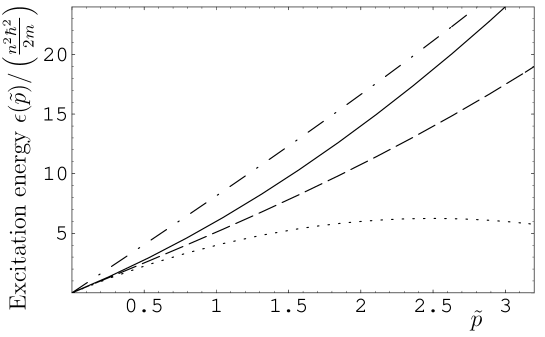
Figure 3: Shown are excitation energies in the thermodynamic limit at $\gamma=16.3$. The full and dotted lines are the excitations within the current Kohn-Sham approach of type I and II from Eqs. (18) and (19), respectively. The dashed line is the result from the linear response of the bosonic LDA (24). The dash-dotted line is the Bogoliubov dispersion (25) which shows the wrong slope at the origin because we are out of the perturbative regime.

3.3 Limits of strong and weak interaction

In the strongly-interacting limit we find $\nu=1$ and $\tilde{N}=N$. In this case $v_{\mathrm{KS}}=0$ and the Kohn-Sham equations become the equations for non-interacting spinless fermions. Due to the Bose-Fermi mapping theorem of Girardeau this gives the correct description of both the full excitation spectrum as well as the (time-dependent) diagonal single-particle densities. In particular we obtain the following equations for type I and II excitations:

$$\epsilon^{\mathrm{I}}(\tilde{p}) = \frac{\hbar^{2}}{2m}n^{2}\tilde{p}\left[2\pi+\tilde{p}\right]$$ (26)

$$\epsilon^{\mathrm{II}}(\tilde{p}) = \frac{\hbar^{2}}{2m}n^{2}\tilde{p}\left[2\pi-\tilde{p}\right]$$ (27)

It is interesting to note that the single-mode equation (1), which here is exactly the equation studied by Kolomeisky [17], does not have the correct limit of Eq. (26). Instead we find

$$\hbar\omega=\frac{\hbar^{2}}{2m}n^{2}\sqrt{\tilde{p}^{2}(\tilde{p}^{2}-2\pi^{2})}.$$ (28)

This limit underestimates the type I excitation energy. It has been suggested in Ref. [17] to link dark solitary waves in the single-mode equation to the type II excitations. The dispersion relation, however, gives only qualitative agreement and underestimates the energy at large momenta. We want to stress that our fermionic LDA, on the contrary, yields the exact excitation spectrum in the Tonks-Girardeau limit.

In the limit of weak interactions we should obtain the single-mode equation with

$$\phi(n)=\mu_{\mathrm{LL}}(n),$$ (29)

as was discussed in the context of the derivation of the Kohn-Sham equations. It was also discussed that the LDA approach for finite interactions followed in the main part of the paper cannot describe the limit of the Bose condensate with a single occupied mode correctly. Indeed it can be seen that Eq. (18) does not reduce to the Bogoliubov form (25) for small $\gamma$, although it has the correct low- and high-energy asymptotics. In order to obtain this limit correctly, a finite size correction should be added to the density functional.

3.4 Static density profiles in the Thomas-Fermi approximation

A consistency check for the static density profiles found from the fermionic LDA can be derived from applying a Thomas-Fermi approximation. The idea is to treat the Kohn-Sham model system of Eq. (9) as non-interacting Fermions (equivalent to a Tonks gas) in the external potential $v_{\mathrm{ext}}(x)+v_{\mathrm{KS}}^{\mathrm{LDA}}(x)$. Approximating now the density by the Thomas-Fermi approximation or hydrodynamic LDA as in Ref. [22] leads to exactly the same equations for the density as the Thomas-Fermi approximation for the original system of interacting bosons discussed in Ref. [22]. This result is independent of the specific choice of $\tilde{N}$ and provides a check for the consistency of the LDA between the different model systems.

4 Conclusions

In this paper we have devised a variational scheme based on Kohn-Sham DFT to calculate ground-state properties and time-dependent processes in the system of 1D bosons with short-range interaction. The scheme will be particularly useful for the regime of strong interaction where fermionization is important and bosonic perturbation theory ceases to be applicable. In contrast to the previously suggested nonlinear Schrödinger equation of Kolomeisky [17], our theory has the correct strong-interaction limit for the density and for ground-state and excitation energies. The degree of fermionization in the model is determined by requiring consistency of the low-energy, low-momentum excitation spectrum. Employing the local-density approximation yields a parameter-free model. Interesting applications and test cases may arise in situation where coherence properties and long-wavelength excitations are important. Due to the construction of our model, it is best suited for situations with a large number of bosons and almost homogeneous densities. A specific example may be the study of shock waves in the homogeneous gas as studied by Damski [27, 38]. In the decay of a shock wave, the usual bosonic LDA fails due to the fact that coherence is overestimated. Exact results are only available for the Tonks-Girardeau limit so far. For finite interaction strengths, our fermionic LDA can make predictions about the importance of coherences and numerical studies of this problem are under way. Another situation where the current theory can be applied is the 1D Bose gas in a weak optical lattice. Interesting questions to study are the nature of excitations and the phase diagram as well as a comparison to the predictions of bosonic LDA.

The DFT scheme studied in this paper is based on the careful choice of the kinetic energy functional determined by the Kohn-Sham auxiliary independent-particle system and the rest of the functional was approximated in the ALDA. The next logical step to improve performance of our model is to go beyond the ALDA and employ standard correction schemes based on current-density functional theory [4, 5].

Appendix A Linear response equations

Following the standard scheme of linear response theory [33] we introduce a time-dependent perturbation

$$v_{\mathrm{ext}}(x,t)=v_{\mathrm{ext}}(x)+\lambda[f^{+}(x)e^{-i\omega t}+f^{-}(x)e^{-i\omega t}]$$

in Eq. (10) where $\lambda$ is small. We look for solutions of Eq. (10) through first order in $\lambda$. To zeroth order we obtain the stationary equation (9). Up to first order we expect to find solutions of the form

$$\varphi_{h}(x,t)=\left\{\varphi_{h}(x)+\lambda\sum_{p\not\in}(X_{hp}e^{-i\omega t}+Y^{*}_{hp}e^{i\omega t})\varphi_{p}(x)\right\}e^{\frac{-i\epsilon_{h}t}{\hbar}}$$ (30)

Here, the linear response of the occupied orbitals can be expanded in terms of unoccupied ($\not\in$) orbitals because the time-evolution according to the Kohn-Sham equations preserves the orthonormality of the occupied orbitals to every order in $\lambda$. Substituting the expression (30) into the time-dependent equation (10) and equating the first order terms with different time-dependence separately and finally setting $f^{\pm}=0$ yields the following equations for small-amplitude free oscillations around the stationary state:

$$\sum_{h^{\prime}\in,p^{\prime}\not\in}({\mathcal{L}}_{hph^{\prime}p^{\prime}}X_{h^{\prime}p^{\prime}}+{\mathcal{M}}_{hph^{\prime}p^{\prime}}Y_{h^{\prime}p^{\prime}}) = \hbar\omega X_{hp}$$ (31)

$$\sum_{h^{\prime}\in,p^{\prime}\not\in}({\mathcal{L}}^{*}_{hph^{\prime}p^{\prime}}Y_{h^{\prime}p^{\prime}}+{\mathcal{M}}^{*}_{hph^{\prime}p^{\prime}}X_{h^{\prime}p^{\prime}}) = -\hbar\omega Y_{hp}$$ (32)

In the basis of stationary Kohn-Sham orbitals [i.e. solutions of Eq. (9)] the matrices read

$${\mathcal{L}}_{hph^{\prime}p^{\prime}} = (\epsilon_{p}-\epsilon_{h})\delta_{pp^{\prime}}\delta_{hh^{\prime}}+\nu v^{\prime}_{ph^{\prime}p^{\prime}h}$$ (33)

$${\mathcal{M}}_{hph^{\prime}p^{\prime}} = \nu v^{\prime}_{pp^{\prime}h^{\prime}h},$$ (34)

where

$$v^{\prime}_{ijkl}=\int\varphi^{*}_{i}(x)\varphi^{*}_{j}(x)\frac{dv_{\mathrm{KS}}}{dn}\Big{|}_{n(x)}\varphi_{k}(x)\varphi_{l}(x)\;dx.$$ (35)

A simple basis transformation may be applied to rewrite Eqs. (33) to (35) in a different basis, e.g. the coordinate representation. For the specific case of the bosonic LDA with $\tilde{N}=1$ we find the Bogoliubov–de Gennes equations of Ref. [18]. In the limit $\gamma\ll 1$ the regular Bogoliubov–de Gennes equations of Gross-Pitaevskii theory are recovered.

For studying the homogeneous system where $v_{\mathrm{ext}}=0$ and $n$ is constant we introduce the usual box quantization with $\phi_{m}(x)=e^{ik_{q}x}/\sqrt{L}$ and $k_{q}=2\pi q/L$. We find

$$\epsilon_{i}=\frac{\hbar^{2}k_{i}^{2}}{2m}+v_{\mathrm{KS}}$$

and $v_{ijkl}=\delta_{i-k,j-l}v^{\prime}_{\mathrm{KS}}/L$ with $v^{\prime}_{\mathrm{KS}}\equiv dv_{\mathrm{KS}}/dn$. Due to translational symmetry the matrix equations block and it makes sense to label the blocks according to the momentum transfer $\hbar k_{p}-\hbar k_{h}=2\pi q\hbar/L$. With defining ${\mathcal{L}}^{q}_{p,p^{\prime}}={\mathcal{L}}_{(p-q)p,(p^{\prime}-q)p^{\prime}}$ we obtain

$${\mathcal{L}}^{q}_{p,p^{\prime}} = (\epsilon_{p}-\epsilon_{p-q})\delta_{p,p^{\prime}}+\frac{\nu v^{\prime}_{\mathrm{KS}}}{L}$$ (36)

$${\mathcal{M}}^{q}_{p,p^{\prime}} = \frac{\nu v^{\prime}_{\mathrm{KS}}}{L}$$ (37)

Due to the presence of the Fermi sphere there are restrictions on the possible values of the indices as $k_{p}$ always has to be outside and $k_{p-q}$ has to be inside.

We now consider the two cases $q=1,2$ explicitely in order to calculate the slopes of both the type I and type II excitation branches at zero momentum. For $q=1$ corresponding to the smallest possible momentum transfer, the matrices ${\mathcal{L}}$ and ${\mathcal{M}}$ have one entry each and Eqs. (31) and (32) can be recast as a 2 by 2 matrix eigenvalue equation. This equation can be solved easily to yield the eigenvalues $\hbar\omega_{1}$ and $-\hbar\omega_{1}$, where $(\hbar\omega_{1})^{2}=\alpha^{2}+2\alpha\nu v^{\prime}_{\mathrm{KS}}/L$ with $\alpha=\hbar^{2}N2\pi^{2}/(mL^{2}\nu)$ and only the positive solution is physically relevant. Using Eqs. (12) and (8) we find that $\hbar\omega_{1}/p_{1}=c_{s}$ where $p_{1}=2\pi\hbar/L$ is the momentum transfer for this excitation and $c_{s}$ is the speed of sound in the Lieb-Liniger model given by Eq. (20). We would like to point out that this result is independent of $\nu$ and can be traced back to the compressibility sum rule which is granted by the LDA.

We are now going to check this result for the speed of sound by calculating the energies for the next larger momentum transfer with $q=2$ where 2 particle-hole excitations give the first possibility to have different slopes for the type I and type II excitation branches. If both branches have the same slope and yield the same speed of sound, the energy difference between these two excitations should vanish in the thermodynamic limit. We have solved the eigenvalue equations (31) and (32) which are 4 by 4 with a specific symmetry. We omit the lengthy expressions but note the following observations: One of the solutions is independent of $\nu$ and gives the speed of sound as in Eq. (20) up to order $1/L$. The other solution does depend on $\nu$ and for the difference between the squared slopes we find

$$\left[(\hbar\omega_{2}^{(1)})^{2}-(\hbar\omega_{2}^{(2)})^{2}\right]/p_{2}^{2}=\frac{n}{2m}v^{\prime}_{\mathrm{KS}}+\mathcal{O}(1/L).$$ (38)

We see that this term remains finite in the thermodynamic limit unless $v^{\prime}_{\mathrm{KS}}$ vanishes, which gives a stringent criterion for the choice of $\nu=N/\tilde{N}$ as discussed in Section 2.4. If the criterion of vanishing $v^{\prime}_{\mathrm{KS}}$ is violated, the model will not only develop phonon branches with different speed of sound but additionally mean-field instabilities may occur as indicated by complex eigenvalues of the linear response equations. In the thermodynamic limit of the homogeneous case this occurs whenever $\tilde{N}$ is larger than the value determined by Eq. (14).

References

References

- [1] P. Hohenberg and W. Kohn, Phys. Rev. 136, B864 (1964).
- [2] W. Kohn and L. J. Sham, Phys. Rev. 140, A1133 (1965).
- [3] E. Runge and E. K. U. Gross, Phys. Rev. Lett. 52, 997 (1984).
- [4] G. Vignale and W. Kohn, Phys. Rev. Lett. 77, 2037 (1996).
- [5] G. Vignale, C. A. Ullrich, and S. Conti, Phys. Rev. Lett. 79, 4878 (1997).
- [6] M. D. Girardeau, J. Math. Phys. 1, 516 (1960).
- [7] T. Cheon and T. Shigehara, Phys. Rev. Lett. 82, 2536 (1999).
- [8] E. H. Lieb and W. Liniger, Phys. Rev. 130, 1605 (1963).
- [9] E. H. Lieb, Phys. Rev. 130, 1616 (1963).
- [10] V. E. Korepin, N. M. Bogoliubov, and A. G. Izergin, Quantum Inverse Scattering Method and Correlation Functions (University Press, Cambridge, 1993).
- [11] M. Olshanii, Phys. Rev. Lett. 81, 938 (1998).
- [12] D. Petrov, G. Shlyapnikov, and J. Walraven, Phys. Rev. Lett. 85, 3745 (2000).
- [13] F. D. M. Haldane, Phys. Rev. Lett. 60, 635 (1988).
- [14] B. Sutherland, Phys. Rev. A 4, 2019 (1971).
- [15] A. Griffin, Can. Journ. Phys. (Brockhouse issue) 73, 755 (1995).
- [16] G. S. Nunes, Journal of Physics B: Atomic, Molecular and Optical Physics 32, 4293 (1999).
- [17] E. B. Kolomeisky, T. J. Newman, J. P. Straley, and X. Qi, Phys. Rev. Lett. 85, 1146 (2000).
- [18] P. Öhberg and L. Santos, Phys. Rev. Lett. 89, 240402 (2002).
- [19] Y. E. Kim and A. L. Zubarev, Phys. Rev. A 67, 015602 (2003).
- [20] M. L. Chiofalo, A. Minguzzi, and M. P. Tosi, Physica B 254, 188 (1998).
- [21] M. L. Chiofalo and M. P. Tosi, Europhys. Lett. 53, 162 (2001).
- [22] V. Dunjko, V. Lorent, and M. Olshanii, Phys. Rev. Lett. 86, 5413 (2001).
- [23] C. Menotti and S. Stringari, Phys. Rev. A 66, 043610 (2002).
- [24] A. L. Fetter and A. A. Svidzinsky, J. Phys.: Condens. Matter 13, R135 (2001).
- [25] A. Lenard, J. Math. Phys. 7, 930 (1964).
- [26] M. D. Girardeau and E. M. Wright, Phys. Rev. Lett. 84, 5239 (2000).
- [27] B. Damski, Shock waves in ultracold Fermi (Tonks) gases, preprint cond-mat/0306394, 2003.
- [28] V. N. Popov, Functional Integrals in Quantum Field Theory and Statistical Physics (Reidel, Dordrecht, 1983).
- [29] P. P. Kuhlish, S. V. Manakov, and L. D. Fadeev, Theor. Math. Phy. 28, 38 (1976).
- [30] A. D. Jackson and G. M. Kavoulakis, Phys. Rev. Lett. 89, 070403 (2002).
- [31] S. Komineas and N. Papanicolaou, Phys. Rev. Lett. 89, 070402 (2002).
- [32] M. Levy, J. P. Perdew, and V. Sahni, Phys. Rev. A 30, 2745 (1984).
- [33] D. J. Thouless, The Quantum Mechanics of Many-Body Systems (Academic Press, New York, 1972).
- [34] M. D. Girardeau and E. M. Wright, Phys. Rev. Lett. 87, 210401 (2001).
- [35] M. Schwartz, Phys. Rev. B 15, 1399 (1977).
- [36] F. D. M. Haldane, Phys. Rev. Lett. 47, 1840 (1981).
- [37] C. N. Yang and C. P. Yang, J. Math. Phys. 10, 1115 (1969).
- [38] B. Damski, Formation of shock waves in a Bose-Einstein condensate, preprint cond-mat/0309421, 2003.