Shock in a Branching-Coalescing Model with Reflecting Boundaries

Abstract

A one-dimensional branching-coalescing model is considered on a chain of length $L$ with reflecting boundaries. We study the phase transitions of this model in a canonical ensemble by using the Yang-Lee description of the non-equilibrium phase transitions. Numerical study of the canonical partition function zeros reveals two second-order phase transitions in the system. Both transition points are determined by the density of the particles on the chain. In some regions the density profile of the particles has a shock structure.

One-dimensional driven lattice gases are models of particles which diffuse, merge and separate with certain probabilities on a lattice with open, periodic or reflecting boundaries. In the open boundaries case the particles are allowed to enter or leave the system from both ends or only one end of the chain. In the reflecting boundaries or periodic boundary cases the number of particles will be a conserved quantity provided that no other reactions other than the diffusion of particles take place. In the stationary state, these models exhibit a variety of interesting properties such as non-equilibrium phase transitions and spontaneous symmetry breaking which cannot be found in equilibrium models (see [1] and references therein). Different applications are also found for such models which include the kinetics of biopolymerization [2] and traffic flow modelling [3]. These models have also allowed the study of shocks i.e. discontinuities in the density of particles over a microscopic region. Over the last decade people have studied the shocks in one-dimensional driven-diffusive models with open and periodic boundary conditions. A prominent example of such models with open boundary is the Asymmetric Simple Exclusion Process (ASEP) in which the particles enter the system from the left boundary, diffuse in the bulk and leave the chain from the right boundary with certain rates [4]. For specific tuning of injection and extraction rates a shock might appear in the system which moves with a constant velocity towards the boundaries. The ASEP has also been studied on a ring in the presence of a second class particle called the impurity [5, 6, 7]. In this case the impurity will track the shock front with a constant velocity which is determined by the reaction rates of the model. The shocks in the models with reflecting boundaries have not been studied yet.
In the present letter we study the phase transitions in a one-dimensional branching-coalescing model with reflecting boundaries in which the particles diffuse, coagulate and decoagulate on a lattice of length $L$. The reaction rules are specifically as follows:

$$\begin{array}[]{llll}\mbox{Diffusion to the left:}&&\emptyset+A\rightarrow A+\emptyset&\mbox{with rate}\;\;q\\ \mbox{Diffusion to the right:}&&A+\emptyset\rightarrow\emptyset+A&\mbox{with rate}\;\;q^{-1}\\ \mbox{Coalescence to the left:}&&A+A\rightarrow A+\emptyset&\mbox{with rate}\;\;q\\ \mbox{Coalescence to the right:}&&A+A\rightarrow\emptyset+A&\mbox{with rate}\;\;q^{-1}\\ \mbox{Branching to the left:}&&\emptyset+A\rightarrow A+A&\mbox{with rate}\;\;\Delta q\\ \mbox{Branching to the right:}&&A+\emptyset\rightarrow A+A&\mbox{with rate}\;\;\Delta q^{-1}\\ \end{array}$$ (1)

in which $A$ and $\emptyset$ stand for the presence of a particle and a hole respectively. It is assumed that there is no injection or extraction of particles from the boundaries. We will also assume that the number of particles on the chain is a conserved quantity. This model was first introduced and treated in continuum approximation in [8, 9, 10, 11]. It was then studied using the Empty Interval Method (EIM) in [12]. In this formalism the physical quantities such as the density of particles are calculated from the probabilities to find empty intervals of arbitrary length. Later this model was studied using so-called the Matrix Product Formalism (MPF) [13]. According to this formalism the stationary probability distribution function of the system is written in terms of the products of non-commuting operators $E$ and $D$ and the vectors $|V\rangle$ and $\langle W|$ as follows

$$P(\tau_{1},\cdots,\tau_{L})=\frac{1}{Z_{L}}\langle W|\prod_{i=1}^{L}(\tau_{i}D+(1-\tau_{i})E)|V\rangle.$$ (2)

Each site of the lattice is occupied by a particle ($\tau_{i}=1$) or is empty ($\tau_{i}=0$). The factor $Z_{L}$ in (2) is a normalization factor. The operators $D$ and $E$ stand for the presence of particles and holes respectively and besides the vectors $|V\rangle$ and $\langle W|$ should satisfy the following quadratic algebra [13]

$$\begin{array}[]{l}[E,\bar{E}]=0\\ \bar{E}D-E\bar{D}=q(1+\Delta)ED-\frac{1}{q}DE-\frac{1}{q}D^{2}\\ \bar{D}E-D\bar{E}=-qED+\frac{1+\Delta}{q}DE-qD^{2}\\ \bar{D}D-D\bar{D}=-q\Delta ED-\frac{\Delta}{q}DE+(q+\frac{1}{q})D^{2}\\ \langle W|\bar{E}=\langle W|\bar{D}=0\\ \bar{E}|V\rangle=\bar{D}|V\rangle=0.\end{array}$$ (3)

The operators $\bar{D}$ and $\bar{E}$ are auxiliary operators and do not enter into calculating (2). Having a representation for the quadratic algebra (3) one can easily compute the steady state weights of any configuration of the system using (2). It has been shown that (3) has a four-dimensional representation [13]. For $q^{2}\neq 1+\Delta$ we have

$$\begin{array}[]{c}D=\left(\begin{array}[]{cccc}0&0&0&0\\ 0&\frac{\Delta}{1+\Delta}&\frac{\Delta}{1+\Delta}&0\\ 0&0&\Delta&0\\ 0&0&0&0\end{array}\right),E=\left(\begin{array}[]{cccc}\frac{1}{q^{2}}&\frac{1}{q^{2}}&0&0\\ 0&\frac{1}{1+\Delta}&\frac{1}{1+\Delta}&0\\ 0&0&1&\frac{1}{q^{2}}\\ 0&0&0&\frac{1}{q^{2}}\end{array}\right),|V\rangle=\left(\begin{array}[]{c}a\\ 0\\ q^{2}\\ q^{2}-1\end{array}\right)\\ \langle W|=\Bigl{(}1-q^{2},1,0,b\Bigr{)}\end{array}$$ (4)

in which $a$ and $b$ are arbitrary constants. The matrix representations for $\bar{D}$ and $\bar{E}$ are also given in [13]. Both EIM and MPA approaches showed that the model has two different phases: a low-density phase for $q^{2}>1+\Delta$ and a high-density phase for $q^{2}<1+\Delta$ and a phase transition takes place at the critical point where $q^{2}=1+\Delta$. In the low-density and the hight-density regions the density profile of the particles on the chain is an exponential function while on the coexistence line it changes linearly along the lattice.
Recently this model has been studied under the open boundary conditions on a specific manifold of the parameters of the system [20]. It is shown that if the particles are injected and extracted from the left boundary with the rates $\alpha$ and $\beta$ respectively then the model has the same phase structure provided that $\alpha=(q^{-1}-q+\beta)\Delta$. In the latter case the operators $D$ and $E$ and also the vectors $\langle W|$ and $|V\rangle$ have two-dimensional representations. The only difference is that for the reflecting boundary conditions the system involves three different length scales while for the open boundary conditions it is characterized by one length scale. Moreover, it has been shown that in the open boundary case the probability distribution function of the system can be written in terms of superposition of Bernoulli shock measures [19]. For the open boundary case if we fix the density of particles, for example by working in a canonical ensemble, we can see the real shock structures in the density profile of particles. In this case the system will also have two different phases: a low-density phase and a jammed-phase where the shocks evolve in the system. These phases are specified by the density of particles and are separated by a second-order phase transition [21].
A natural question that might arise is whether or not we can see the shocks in our branching-coalescing model defined by (1) with the reflecting boundaries. To answer this question we will study the model with reflecting boundaries in a canonical ensemble where the number of particles on the chain is equal to $M$ so that the density of particles $\rho=\frac{M}{L}$ remains constant. We will then investigate the phase transitions and the density profile of particles on the chain. Recently it has been shown that the classical Yang-Lee theory [14, 15] can be applied to the one-dimensional out-of-equilibrium systems in order to study the possible phase transitions of these models [16, 17, 18, 20, 21]. According to this theory in the thermodynamic limit, the zeros of the canonical or grand canonical partition function, as a function of an intensive variable of the system, might approach the real positive axis of that parameter at one or more points. Depending on how these zeros approach the real positive axis the system might have one or more phase transition of different orders. If the zeros intersect the real positive axis at a critical point at an angle $\frac{\pi}{2n}$, then $n$ will be the order of phase transition at that point [16].
Let us define the canonical partition of our model using the MPF as follows

$$Z_{L,M}=\sum_{\{\tau_{i}=0,1\}}\delta(M-\sum_{i=1}^{L}\tau_{i})\langle W|\prod_{i=1}^{L}(\tau_{i}D+(1-\tau_{i})E)|V\rangle$$ (5)

in which $M$ and $L$ are the number of particles and the length of the system respectively and $\delta(\cdots)$ is the ordinary Kronecker delta function $\delta_{x,0}$. Using the matrix representations $D$, $E$, $\langle W|$ and $|V\rangle$ given by (4) we have been able to calculate the canonical partition of this model (5) and its zeros numerically. One can use MATHEMATICA to calculate $\langle W|(E+xD)^{L}|V\rangle$ for arbitrary $q$ and $\Delta$ and finite $L$ in which $x$ is a free parameter. The result will be a polynomial of $x$. The coefficient $x^{M}$ in this polynomial gives the canonical partition function of the system. Formally we can write

$$Z_{L,M}=Coefficient[\langle W|(E+xD)^{L}|V\rangle,M]$$ (6)

in which $Coefficient[Expr,n]$ gives the coefficient of $x^{n}$ in the polynomial $Expr$. In Fig. 1 we have plotted the numerical estimates for the zeros of $Z_{L,M}$ obtained from (6) on the complex-$q$ plane for $L=80$, $M=42$. The canonical partition function (6) has $4(L-M)$ zeros in the complex-$q$ plane. We have found that for large $L$ and $M$ the locations of these zeros are not sensitive to the value of $\Delta$. We have also calculated the numerical estimates for the roots of (6) as a function of $\Delta$ for fixed values of $q$. It turns out that (6), as a function of $\Delta$, does not have any positive root; therefore, we expect that the phase transition points do not depend on $\Delta$.

Figure 1: Plot of the numerical estimates for the canonical partition function zeros obtained from (6) for $L=80$ and $M=42$.

As can be seen in Fig. 1 the zeros lie on two different curves and accumulate towards two different points on the positive real-$q$ axis. By extrapolating the real part of the nearest roots to the positive real-$q$ axis for large $L$ and $M$, we have found that the transition points are $q_{c}=\frac{1}{\sqrt{1-\rho}}\;\;(1<q_{c}<\infty)$ and $q_{c}^{\prime}=\sqrt{1-\rho}\;\;(0<q_{c}^{\prime}<1)$. As $\rho\rightarrow 0$ the two curves lie on each other and we will find only one transition point at $q_{c}=q_{c}^{\prime}=1$. It appears also that the zeros on both curves approach the real-$q$ axis at an angle $\frac{\pi}{4}$ (the smaller angle). This predicts two second-order phase transitions at $q_{c}$ and $q_{c}^{\prime}$. The reason that the system has two phase transitions can easily be understood. The parameter $q$ determines the asymmetry of the system and for any $q$ the system is invariant under the following transformations

$$q \longrightarrow q^{-1}$$

$$i \longrightarrow L-i+1.$$ (7)

Therefore, one can expect to distinguish two critical points which are related according to the symmetry of the system.
Let us now study the density profile of particles on the chain $\rho(i)$ in each phase. The density of particles at site $i$ is defined as

$$\rho(i)=\frac{\sum_{{\mathcal{C}}}\tau_{i}P(\tau_{1},\cdots,\tau_{L})}{\sum_{{\mathcal{C}}}P(\tau_{1},\cdots,\tau_{L})}$$ (8)

in which ${\mathcal{C}}$ is any configuration of the system with fixed number of particles $M$ and $P(\tau_{1},\cdots,\tau_{L})$ is given by (2). It can be verified that the density profile of the particles $\rho(i)$ can be written as

$$\begin{array}[]{c}\rho(i)=\frac{1}{Z_{L,M}}\\ \sum_{k=0}^{M-1}\langle W|Coefficient[C^{i-1},k]\;D\;Coefficient[C^{L-i},M-k-1]|V\rangle\end{array}$$ (9)

where we have defined $C:=E+xD$. Now one can use the matrix representation (4) to calculate (9) using MATHEMATICA. In Fig. 2 we have plotted (9) for two different values of $q$ with $L=60$ and $M=36$.

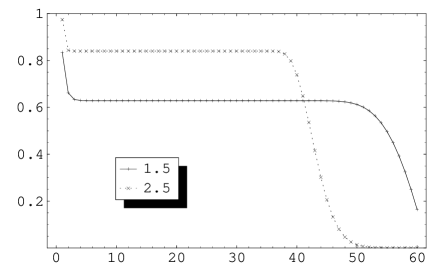
Figure 2: Plot of the density profile of the particles (9) on a chain of length $L=60$ for $M=36$ and two values of $q\;(q>1)$ above and below the critical point $q_{c}=1.581$.

For this choice of the parameters the transition points are $q_{c}=1.581$ and $q_{c}^{\prime}=0.633$. The density of particle has two general behaviors for $q>1$. For $q>q_{c}$ and in the thermodynamic limit ($L\rightarrow\infty,M\rightarrow\infty,\rho=\frac{M}{L}$) the density profile of particles is a shock in the bulk of the chain; while in the close vicinity of the left boundary, it increases exponentially. The density of particles in the hight-density region of the shock is equal to $\rho_{High}=1-q^{-2}$. This region is separated by a rather sharp interface from the low-density region in which the density of particles is equal to $\rho_{Low}=0$. The low-density region is extended over $(1-\frac{\rho}{1-q^{-2}})L$ sites. This can be seen in Fig. 2 for $q=2.5$; however, the reason that the shock interface is not sharp is that our calculations are not done in real thermodynamic limit. One should expect that the shock front becomes sharper and sharper as the length of the system $L$ and also the number of particles on the chain $M$ increase. For $1<q<q_{c}$ the density of particles in the bulk of the chain is constant equal to $\rho$, it drops near the right boundary exponentially and increases exponentially in the close vicinity of the left boundary. The exponential behavior of the density profile of particles near the boundaries in this phase is due to the finiteness of the representation of the algebra (3). It is known that if the associated quadratic algebra of the model has finite dimensional representations, the density-density correlation functions cannot have algebraic behaviors [13]. At $q=1$ one finds $\rho(i)=\rho$. The density profile of particles in the region $q<1$ is related to that of $q>1$ through (Shock in a Branching-Coalescing Model with Reflecting Boundaries) that is

$$\rho(i,q)=\rho(L-i+1,q^{-1}).$$ (10)

One can also study this model on a ring of length $L$ with periodic boundary conditions. Let us assume that the number of particles and therefore their density fluctuates and is not a constant. In this case the probability of finding the system in a specific configuration ${\mathcal{C}}=\{\tau_{1},\cdots,\tau_{L}\}$ should be obtained from

$$P(\tau_{1},\cdots,\tau_{L})=\frac{1}{Z_{L}}tr[\prod_{i=1}^{L}(\tau_{i}D+(1-\tau_{i})E)].$$ (11)

in which $tr[\cdots]$ is the trace of the products of matrices. The normalization factor $Z_{L}$ can be obtained from the fact that $\sum_{\mathcal{C}}P({\mathcal{C}})=1$. This function plays the role of the grand canonical partition function of the system. One can easily check that the quadratic algebra associated to the periodic boundary condition case is the same as (3) except the boundary terms which contain the vectors $|V\rangle$ and $\langle W|$; therefore, we can still use the algebra (3) and its representation (4) to calculate (11). As we mentioned the grand canonical partition function of the system can be defined as

$$Z_{L}=\sum_{\{\tau=0,1\}}tr[\prod_{i=1}^{L}(\tau_{i}D+(1-\tau_{i})E)]=tr[(E+D)^{L}].$$ (12)

This can easily be calculated and we find

$$Z_{L}=1+q^{-2L}+q^{2L}+(1+\Delta)^{L}.$$ (13)

The study of the zeros of (13) as a function of $q$ in the thermodynamic limit $L\rightarrow\infty$ shows that they approach the positive real-$q$ axis at two different points $q_{c}=\sqrt{1+\Delta}\;(1<q_{c}<\infty)$ and $q_{c}^{\prime}=\frac{1}{\sqrt{1+\Delta}}\;(0<q_{c}^{\prime}<1)$. Moreover, the zeros approach the positive real-$q$ axis at angle $\frac{\pi}{2}$; therefore, unlike the reflecting boundaries case both phase transitions in this case are of first-order. In the steady state the density profile of the particles on the ring is flat and equal to $\rho(i)=\frac{\Delta}{1+\Delta}$ for $q_{c}^{\prime}<q<q_{c}$ and $\rho(i)=0$ for $q>q_{c}$ and $q<q_{c}^{\prime}$. One can take the total density of particles on the ring as an order parameter and since it changes discontinuously over the transition points, as the Yang-Lee theory predicts, the phase transitions are of first-order. One should note that in comparison to the reflecting boundaries case not only the geometry of the model is changed but also the number of particles in this case in not a conserved quantity. This means that we should not expect the transitions in these models to be similar even if we take the thermodynamic limit $L\rightarrow\infty$. The reason for the existence of two phase transition points is again the symmetry of the model.
In this letter we have studied a branching-coalescing model in which particles hop, coagulate and decoagulate on one-dimensional lattice of length $L$. We have restricted ourself to the case where the total number of particles on the chain is constant. For this we have worked in the canonical ensemble in which the number of particles $M$ is fixed; therefore, the density of particles on the chain $\rho=\frac{M}{L}$ is constant. The Yang-Lee theory predicts that the model has two second-order phase transitions. Both phase transition points are determined by the density of particles on the system $\rho$. The study of the mean particle concentration at each site of the chain for $q>1$ shows that the density profile of the particles has a shock-like structure in the region $q>q_{c}=\frac{1}{\sqrt{1-\rho}}$. The exception is near the left boundary where the density of particles increases exponentially. This is the first time that shocks are seen in one-dimensional reaction-diffusion models with reflecting boundaries. In the region $1<q<q_{c}=\frac{1}{\sqrt{1-\rho}}$ the density profile of the particles is constant in the bulk of the chain; however, near the left (right) boundary it increases (decreases) exponentially. The exact form of the correlation lengths is under investigation. Our numerical investigations also show that the width of the shock scales as $L^{-\nu}$ with $\nu=\frac{1}{2}$. In the thermodynamic limit $L\rightarrow\infty$ the shock width goes to zero and one finds a very sharp shock interface. Since the system is invariant under the transformation (Shock in a Branching-Coalescing Model with Reflecting Boundaries), the density profile of the particles for $q<1$ can be obtained from (10). We also studied the periodic boundary case and found that the system possess two first-order phase transitions which are determined by the values of $\Delta$ for fixed value of $q$. In this case the density profile of particles is flat everywhere on the lattice and is either equal to $\frac{\Delta}{1+\Delta}$ or zero. The formulas (6) and (9) provide us with a simple and general tool for numerical study of the phase transitions and also the particle concentration behaviors of one-dimensional stochastic models in canonical ensemble for which a finite- or infinite-dimensional representation of the associate algebra exists.

References

- [1] G.M. Schütz Phase Transitions and Critical Phenomena vol 19 ed C. Domb and J. Lebowitz (New York: Academic Press 1999)
- [2] C.T. McDonald, J.H. Gibbs and A.C. Pipkin Biopolymers 6, 1(1968)
- [3] D. Chowdhury, L. Santen and A. Schadschneider Phys. Rep. 329 199(200))
- [4] B. Derrida, M.R. Evans, V. Hakim and V. Pasquier J. Phys. A: Math. Gen. A 26 1493 (1993)
- [5] K. Mallick J. Phys. A: Math. Gen. A 29 5375 (1996)
- [6] H-W. Lee, V. Popkov and D. Kim J. Phys. A: Math. Gen. A 30 8497 (1997)
- [7] F.H. Jafarpour J. Phys. A: Math. Gen. A 33 8673(2000)
- [8] C. R. Doering and D. ben-Avraham Phys. Rev. A 38 3055 (1988)
- [9] M.A. Burschka, C.R. Doering and D. ben-Avraham Phys. Rev. Lett. 63 700 (1989)
- [10] D. ben-Avraham, M.A. Burschka and C.R. Doering J. Stat. Phys. 60 695 (1999)
- [11] C. R. Doering, M.A. Burschka and W. Horsthemke J. Stat. Phys. 65 953 (1991)
- [12] H. Hinrichsen, K. Krebs and I. Peschel Z. Phys. B 100 105(1996)
- [13] H. Hinrichsen, K. Krebs and I. Peschel J. Phys. A: Math. Gen. A 29 2643 (1996)
-
[14]
C.N. Yang and T.D. Lee Phys. Rev. 87 404(1952)
C.N. Yang and T.D. Lee Phys. Rev. 87 410 (1952) -
[15]
S. Grossmann and W. Rosenhauer Z. Phys. 218 437 (1969)
S. Grossmann and V. Lehmann Z. Phys. 218 449 (1969) -
[16]
R.A. Blythe and M.R. Evans Phys. Rev. Lett. 89 080601 (2002)
R.A. Blythe and M.R. Evans Brazilian Journal of Physics 33 464 (2003) - [17] P.F. Arndt Phys. Rev. Lett. 84 814 (2000)
- [18] F.H. Jafarpour J. Stat. Phys. 113 269 (2003)
- [19] K. Krebs, F.H. Jafarpour and G.M. Schütz New Journal of Physics 5 145.1-145.14 (2003)
- [20] F.H. Jafarpour J. Phys. A: Math. Gen. A 36 7497 (2003)
- [21] F.H. Jafarpour Submitted to the Journal of Phyiscs A: Mathematical and General (2003)