Dual Geometric Worm Algorithm for Two-Dimensional Discrete Classical Lattice Models

Abstract

We present a dual geometrical worm algorithm for two-dimensional Ising models. The existence of such dual algorithms was first pointed out by Prokof’ev and Svistunov Prokof’ev and Svistunov (2001). The algorithm is defined on the dual lattice and is formulated in terms of bond-variables and can therefore be generalized to other two-dimensional models that can be formulated in terms of bond-variables. We also discuss two related algorithms formulated on the direct lattice, applicable in any dimension. These latter algorithms turn out to be less efficient but of considerable intrinsic interest. We show how such algorithms quite generally can be “directed” by minimizing the probability for the worms to erase themselves. Explicit proofs of detailed balance are given for all the algorithms. In terms of computational efficiency the dual geometrical worm algorithm is comparable to well known cluster algorithms such as the Swendsen-Wang and Wolff algorithms, however, it is quite different in structure and allows for a very simple and efficient implementation. The dual algorithm also allows for a very elegant way of calculating the domain wall free energy.

I Introduction

Over the recent decades many powerful Monte Carlo (MC) algorithms have been developed, greatly enhancing the scope and applicability of Monte Carlo techniques. In fact, it is quite likely that these algorithmic advances have, and will continue to have, a far greater impact on the predictive power of Monte Carlo simulations than advances in raw computational capacity, a point that is often overlooked. The continued development of such advanced algorithms is therefore very important. Here we shall mainly be concerned with MC algorithms suitable for the study of lattice models described by classical statistical mechanics. Some of the most notable developments in this field have been the development of cluster algorithms by Swendsen and Wang Swendsen and Wang (1987) and by Wolff Wolff (1989). More recent developments include invaded cluster algorithms Machta et al. (1995) that self-adjust to the critical temperature, flat histogram methods Wang and Landau (2001), focusing on the density of states and techniques performing Monte Carlo sampling of the high temperature series expansion of the partition function Prokof’ev and Svistunov (2001) using worm algorithms Prokof’ev et al. (1998). Two of us recently proposed a very efficient geometrical worm algorithm Alet and Sørensen (2003a, b) for the bosonic Hubbard model. In this algorithm variables are not updated at random but instead a “worm” is propagated through the lattice, at each step choosing a new site to visit with a probability proportional to the relative (among the different sites considered) probability of changing the corresponding variable. The high efficiency of the algorithm stems from the fact that the worm is always moved and it is only through the actual movement that the local environment - the local “geometry” - comes into play. The ideas underlying this algorithm are quite generally applicable and the present paper is concerned with their generalization to classical statistical mechanics models.

As the canonical testing ground for new algorithms we consider the standard ferromagnetic Ising model in two dimensions defined by:

$$H=-J\sum_{<i,j>}s_{i}s_{j},\ \ s_{i}=\pm 1.$$ (1)

Here $<i,j>$ denote the summation over nearest neighbor spins. It is well known that the critical temperature for this model in two dimensions is $k_{B}T_{c}=2J/\log(1+\sqrt{2})=J2.26918\ldots$. When investigating magnetic materials modeled by classical statistical mechanics such as Eq. (1) using Monte Carlo methods one has to take into account the effects of the non-zero auto-correlation time $\tau$ (defined below) that is always present in Monte Carlo simulations. The auto-correlation time describes the correlation between observations of an observable ${\cal O}(t_{0})$ and ${\cal O}(t_{0}+t)$, $t$ Monte Carlo Sweeps (MCS) apart. The auto-correlation time, $\tau$, depends on the simulation temperature and the system size and grows dramatically close to the critical temperature, $T_{c}$, a phenomenon referred to as critical slowing down. At $T_{c}$ the auto-correlation time displays a power-law dependence of the system size, $\tau\sim L^{z_{MC}}$, defining a Monte Carlo dynamical exponent $z_{MC}$. For the well known Metropolis algorithm one estimates Newman and Barkema (1999); Landau and Binder (2000) $z_{MC}\sim 2.1-2.2$. If efficient algorithms, with a very small $z_{MC}$, cannot be found, this scaling renders the Monte Carlo method essentially useless for large lattice sizes since all data will be correlated. It is therefore crucial to develop algorithms with a very small or zero $z_{MC}$. In order to test the proposed algorithms we shall therefore only consider simulations at the critical point since this is where the critical slowing down is the most pronounced and where $z_{MC}$ is defined.

The geometrical worm algorithm Alet and Sørensen (2003a, b) has proven to be very efficient for the study of the bosonic Hubbard model when formulated in terms of currents on the links of the space-time lattice. The estimated $z_{MC}$ is very close to zero Alet and Sørensen (2003b). It is therefore natural to generalize this algorithm to classical models defined in terms of bond-variables. This is done in section III, where a very efficient algorithm formulated directly on the dual lattice is developed. A related dual algorithm was initially described by Prokof’ev and Svistunov Prokof’ev and Svistunov (2001). Our algorithm can be generalized to Potts, clock and other discrete lattice models of which the Ising model is the simplest example. The dual algorithm also allows for a very simple and elegant way of calculating the domain wall free energy directly. In section III we outline how this is done. Regrettably, only in two dimensions is it possible to define such a dual algorithm. In section III we also present a directed version of this algorithm where the probability for the worms to erase themselves is minimized. However, before presenting the dual algorithm it is instructive to consider geometrical worm algorithms defined on the direct lattice. Such an algorithm is described in section II, in both directed and undirected versions. This algorithm is applicable in any dimension but is of less interest due to its poor efficiency. However, from an algorithmic perspective this algorithm is interesting in its own right and it leads naturally to the definition of the dual algorithm. Finally, in section IV we conclude with a number of observations concerning the properties of the algorithms.

II Geometrical Worm Algorithms on the Direct Lattice

The first algorithm we present we shall refer to as the linear worm algorithm. This algorithm is closely related to the geometrical worm algorithms Alet and Sørensen (2003a, b), however, the worms do not form closed loops, instead they form linear strings (a worm) of flipped spins. A major advantage of this algorithm is that we can select the length of the linear worm or even the entire distribution of worm lengths. This could be advantageous for the study of frustrated or disordered models where other cluster algorithms fail due to the fact that too “big” or too “small” clusters are being generated, leading to a significant loss of efficiency.

II.1 Algorithm A (Linear Worms)

We begin with a number of useful definitions: In order to define a working algorithm we consider two configurations of the spins, $\mu$ and $\nu$ related by the introduction of a worm. Let $\mu$ denote the configurations of the spins without the worm, $w$, and $\nu$ the configuration of the spins with the worm. Furthermore, let $s_{1}\ldots s_{W}$ be the sites (or spins) visited by the worm (of length $W$) and let $E_{i}$ denote the energy require to flip the spin at site $s_{i}$ from its position in the configuration $\mu$, with $-E_{i}$ the energy required to flip spin $i$ from its position in $\nu$ to that in $\mu$. Note that $E_{i}$ is defined relative to the spin configuration $\mu$. In the following we shall make extensive use of the activation or local weight for overturning a spin, $A^{E_{i}}_{s_{i}}$. More precisely, $A^{E_{i}}_{s_{i}}$ denotes the weight for flipping $s_{i}$ from its position in $\mu$ to that in $\nu$ and $A^{-E_{i}}_{s_{i}}$ the weight for going in the opposite direction. As we shall see, $A^{E_{i}}_{s_{i}}$ is not uniquely determined. Here, we shall use $A^{E_{i}}_{s_{i}}=\min(1,\exp(-\Delta E_{i}/k_{B}T))$ although other choices would be equally suitable. When the worm is moving through the lattice it will move from the current site $s_{i}$ to a set of neighboring sites $\sigma$ and it becomes necessary to define the normalization $N_{s_{i}}=\sum_{\sigma}A^{E_{i+\sigma}}_{s_{i}+\sigma}$. This normalization is used for choosing the next neighbor to visit among the set $\sigma$ of neighbors.

If one considers the proofs for the geometrical worm algorithms Alet and Sørensen (2003a, b), it is not difficult to see that a generalization to classical statistical models defined on the direct lattice will depend crucially on the fact that the normalization $N_{s_{i}}$ does not depend on the position (up or down) of the spin, $s_{i}$, at the site itself. For the Ising model, defined in Eq. (1), only nearest neighbor interactions are taken into account and we can satisfy this requirement simply by not allowing the worm to move to any of the 4 nearest neighbor sites to the current site $s_{i}$. In principle, one can consider moving the worm to any other sites in the lattice, an aspect of this algorithm of considerable intest. For the case of longer range interactions we would have to restrict the worm to move only to sites that the current spin does not interact with. Note that, since we allow sites on the same sub-lattice to be visited then the $A^{E_{i}}_{s_{i}}$ will depend on the order that we visit the sites since sites neighboring $s_{i}$ could have been visited previously by the worm. As an example of a simple choice for the neighbors we show in Fig 1 an example where the worm can move to 4 neighbors around the current site, excluding the 4 nearest neighbors to the site. When defining the set of neighbors $\sigma$ for the worm to move to from $s_{i}$ one also has to satisfy the trivial property that if $s_{i+1}$ is a neighbor of $s_{i}$ then $s_{i}$ should also be a neighbor of $s_{i+1}$.

We now propose one possible implementation of the geometrical worm algorithm for the Ising model. A set of suitable neighbors to $s_{i}$ is defined as outlined above and at the beginning of the construction of the worm we draw its length, $W$ from a normalized distribution. We refer to this algorithm as linear worms (A). Below we outline the algorithm in pseudo-code.

1. Choose a random starting site, $s_{i=1}$ and with normalized probability a length $W$.

2. Calculate the probability for flipping the spin on that site $A^{E_{1}}_{s_{1}}$ with $A^{E_{i}}_{s_{i}}=\min(1,\exp(-\Delta E_{s_{i}}/k_{B}T))$.

3. Flip the selected spin, $s_{i}$.

4. For each of the $k$ neighbors in the set of neighbors $\sigma$, calculate the weight for flipping, $A^{E_{i+\sigma}}_{s_{i}+\sigma}=\min(1,\exp(-\Delta E_{s_{i}+\sigma}/k_{B}T))$. Calculate the normalization $N_{s_{i}}=\sum_{\sigma}A^{E_{i+\sigma}}_{s_{i}+\sigma}$ and the probabilities $p^{\sigma}_{s_{i}}=A^{E_{i}}_{s_{i}+\sigma}/N_{s_{i}}$.

5. According to the probabilities $p^{\sigma}_{s_{i}}$ select a new site $s_{i+1}$ among the neighbors to go to and increase $i$ by one, $i\to i+1$.

6. If $i<W$ go to 3.

7. Calculate $A^{-E_{W}}_{s_{W}}$ and $\bar{N}_{s_{W}}$ after the worm is constructed and with probability $P_{e}(w)=1-\min(1,A^{E_{1}}_{s_{1}}N_{s_{1}}/(A^{-E_{W}}_{s_{W}}\bar{N}_{s_{W}}))$ erase the constructed worm. Here $A^{E_{1}}_{s_{1}}$ and $N_{s_{1}}$ are calculated before the worm is constructed.

8. Goto 1.

Note that if we decide to construct a worm of length $W=1$ at a given site $s_{1}$ then the above algorithm corresponds to attempting a Metropolis spin-flip at that site.
See appendix A for a proof of the above algorithm.

II.2 Algorithm B (Directed Linear Worms)

It is an obvious advantage to have control over the distribution of the length of the worms. However, if we choose the length of the worm at the start of the construction of the worm as in algorithm A then we allow for the worm to backtrack, thereby erasing itself. We can try to eliminate or rather minimize the probability for the worm to do back-tracking by constructing a directed algorithm. We closely follow the method outlined in reference Alet and Sørensen, 2003b in order to construct a directed algorithm. See also reference Syljuåsen and Sandvik, 2002 for previous work on directed algorithms. Let $\sigma_{m}$ and $\sigma_{n}$ be among the neighbors, ${\bf\sigma}$, of the site $s_{i}$. The above proof of algorithm A does not depend directly on the definition of the probabilities $p^{\sigma_{m}}_{s_{i}}$ and $p^{\sigma_{n}}_{s_{i}}$, but only on their ratio, since they have to satisfy the following relation:

$$\frac{p^{\sigma_{m}}_{s_{i}}}{p^{\sigma_{n}}_{s_{i}}}=\frac{A_{s_{i}+\sigma_{m}}/N_{s_{i}}}{A_{s_{i}+\sigma_{n}}/N_{s_{i}}}=\frac{A_{s_{i}+\sigma_{m}}}{A_{s_{i}+\sigma_{n}}}.$$ (2)

This leaves us considerable freedom since we can define conditional probabilities, $p_{s_{i}}(m|n)$, corresponding to the probability to continue in the direction $\sigma_{m}$ at the site $s_{i}$ if we are coming from $\sigma_{n}$. At a given site we then only need to satisfy

$$\frac{p_{s_{i}}(m|n)}{p_{s_{i}}(n|m)}=\frac{A_{s_{i}+\sigma_{m}}}{A_{s_{i}+\sigma_{n}}}.$$ (3)

If we have $k$ neighbors this defines a $k\times k$ matrix $P$ where the diagonal elements corresponds to the back-tracking probabilities, the probabilities for the worm to erase itself. Previously, we had effectively been using $p_{s_{i}}(m|n)$’s which were independent of the incoming direction, $\sigma_{n}$, since we simply had $p_{s_{i}}(m|n)=A_{s_{i}+\sigma_{m}}/N_{s_{i}}$, corresponding to a matrix $P$ with identical columns. However, the above condition of balance, Eq. (3) leaves sufficient room for choosing very small back-tracking probabilities and in most situations the corresponding diagonal elements of $P$ can be chosen to be zero. If we impose the constraint that the sum of the diagonal elements of $P$ should be minimal the problem of finding an optimal matrix $P$ can be formulated as a standard linear programming problem to which conventional techniques can be applied Alet and Sørensen (2003b).

At a given site $s_{i}$ we choose 4 neighbors, as indicated in Fig. 1 by the open circles $\circ$. The activation at a given neighbor will depend on its 4 nearest neighbors shown as the shaded circles in Fig. 1.

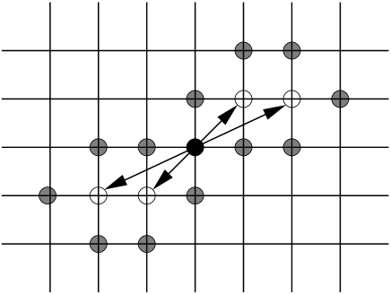
Figure 1: An example of the configuration of the neighbors for algorithm A,B. The current site, $s_{i}$, is indicated by $\bullet$, the neighbors by $\circ$. The activation (weight) at the current site will depend on the spins at the nearest neighbor sites (shaded circles).

Technically, each $p_{s_{i}}(m|n)$ now depends on the position of all the 16 surrounding spins. and hence there are in principle $2^{16}$ possible matrices $P$ at each site. It is therefore not feasible to choose too large a set of neighbors when directing the algorithm. In the absence of disorder, the $2^{16}$ matrices can be tabulated and minimized at the beginning of the simulation and for the isotropic ferromagnetic model at hand it is easy to see that at most 625 different matrices occur.

We can now use the above matrices $P$ for an algorithm that performs directed linear worms of length varying between 1 and $W$. We again assume that a set $\sigma$ of $k$ neighbors has been chosen.

1. Choose a random starting site, $s_{i=1}$ and with normalized probability a length $W$.

2. Calculate the probability for flipping the spin on that site $A^{E_{1}}_{s_{1}}$ with $A^{E_{i}}_{s_{i}}=\min(1,\exp(-\Delta E_{s_{i}}/k_{B}T))$.

3. Flip the selected spin, $s_{i}$.

4. If $s_{i}=s_{1}$ then for each of the $k$ neighbors in the set $\sigma$, calculate the probability for flipping, $A^{E_{i+\sigma}}_{s_{i}+\sigma}=\min(1,\exp(-\Delta E_{s_{i}+\sigma}/k_{B}T))$. Calculate the normalization $N_{s_{i}}=\sum_{\sigma}A^{E_{i+\sigma}}_{s_{i}+\sigma}$ and the probabilities $p^{\sigma}_{s_{i}}=A^{E_{i}}_{s_{i}+\sigma}/N_{s_{i}}$. Else: Depending on the configuration of the nearest neighbors of the $k$ neighbors select the correct (minimized) matrix $P$ and if the worm arrived from direction $\sigma_{n}$ set $p^{\sigma}_{s_{i}}$ equal to the n’th column of $P$.

5. According to the probabilities $p^{\sigma}_{s_{i}}$ select a new site $s_{i+1}$ to go to and increase $i$ by one, $i\to i+1$.

6. If $i<W$ go to 3.

7. Calculate $A^{-E_{W}}_{s_{W}}$ and $\bar{N}_{s_{W}}$ after the worm is constructed and with probability $P_{e}(w)=1-\min(1,A^{E_{1}}_{s_{1}}N_{s_{1}}/(A^{-E_{W}}_{s_{W}}\bar{N}_{s_{W}}))$ erase the constructed worm. Here $A^{E_{1}}_{s_{1}}$ and $N_{s_{1}}$ are calculated before the worm is constructed.

8. Goto 1.

The proof of the above algorithm can be found in appendix B.

II.3 Performance: Algorithms A,B

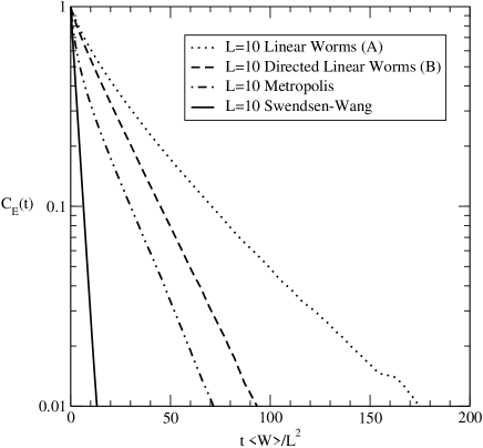
Figure 2: Autocorrelation functions for the energy $C_{E}(t)$ as a function of Monte Carlo time, calculated at $T_{c}$. Shown are results for $L=10$ for the Metropolis, Swendsen-Wang and for the linear worm (A) and directed linear worm (B) algorithms (with uniform worm length). Note that in order to compare the 4 algorithms the time axis has been scaled so that in all cases 1 time step corresponds to an attempted update of all the variables. The autocorrelation functions shown were calculated averaging over 20 million worms (MCS for the metropolis algorithm).

In order to test the performance of algorithms A and B we consider the autocorrelation function $C_{\cal O}(t)$ of an observable ${\cal O}$. This function is defined in the standard way:

$$C_{\cal O}(t)=\frac{\langle{\cal O}(t){\cal O}(0)\rangle-\langle{\cal O}\rangle^{2}}{\langle{\cal O}^{2}{\rangle-\langle{\cal O}\rangle}^{2}}$$ (4)

For a reliable estimate of $C_{\cal O}(t)$ we typically generate 20 million worms. In Fig. 2 we show results for the autocorrelation function for the energy $C_{E}(t)$ for the linear worm algorithms A,B for a system of size $L=10$. In both cases the worm length $W$ was chosen from a uniform distribution. This is compared to $C_{E}(t)$ for the usual single flip Metropolis algorithm and the Swendsen-Wang algorithm. For the latter two algorithms the Monte Carlo time is usually measured in terms of Monte Carlo Sweeps (MCS) where an attempt to update all the $L^{2}$ spins in the lattice has been made. However, for algorithms A and B a worm will on average only attempt to update $\langle W\rangle$ of the $L^{2}$ spins. Hence, if time is measured in terms of generated worms for the worm algorithms it should be rescaled by a factor of $\langle W\rangle/L^{2}$ for a fair comparison to be made with algorithms where Monte Carlo time is measured in MCS. This has been done in Fig. 2. From the results in Fig. 2 it is clear that the efficiency of algorithm A and B is fairly poor and worse than the much simpler Metropolis algorithm. We have checked that this remains true for significantly larger lattices sizes.

The main cause of this poor behavior is the necessity to include a rejection probability $P_{e}$. If a worm on average attempts to update $\langle W\rangle$ spins, we need on average to generate $L^{2}/\langle W\rangle$ worms to complete a MCS. As a rough estimate, let us consider that the worm is accepted with the average probability $p$ and that only a fraction $x$ of the $\langle W\rangle$ attempted spin flips result in an updated spin (a spin can be visited several times). It then follows that on average $pxL^{2}$ are actually flipped in a MCS with the linear worm algorithm. If the average probability for flipping a spin with the Metropolis algorithm is $q$ and if all the spins selected in a MCS are different, the corresponding number for the Metropolis algorithm is $qL^{2}$, presumably of the same order as $pxL^{2}$ and likely larger. The effect of the directed linear worm algorithm is to maximize $x$ as much as possible and it therefore seems unlikely that the linear worm algorithm in its present form can perform better than the Metropolis algorithm unless $p$ also is maximized.

It would be very interesting if algorithms A and B could be modified so that $p\equiv 1$ ($P_{e}\equiv 0$). We have so far been unable to do so. Such a modified algorithm would be significantly more efficient than the Metropolis algorithm (but presumably less efficient than the Swendsen-Wang algorithm). It would be much more versatile and could be of significant interest for frustrated or disordered systems since it would not require the construction of clusters but only of the much simpler worms, the length of which can be chosen.

Even though it is quite interesting to be able to choose the distribution of the worm lengths at the outset, the question arises which distribution of worm lengths will give the most optimal algorithm. In the present work we have chosen a distribution of worm lengths that is uniform between 1 and $2L$, but on general grounds we expect a power-law form for this distribution to be more optimal at the critical point. For the study of Bose-Hubbard models using geometrical worm algorithms it was noted Alet and Sørensen (2003b) that the distribution of the size of the worms follow a power-law with an exponent of approximately 1.37 at the critical point. Hence, in the present case it would appear likely that an optimal power-law distribution of the worm lengths at $T_{c}$ can be found, defining a new “dynamical” exponent. The idea of choosing the distribution of the worm size to optimize the algorithm resembles previous work by Barkema and Newman Barkema and Marko (1993); Newman and Barkema (1996).

In closing this section, we note that it is quite straightforward to define an algorithm on the direct lattice where the worms form closed loops (rings). In this case the length of the worm is determined by the size of the loop. We have tested such algorithms but their performance is even worse than algorithms A and B since the constraint that the initial spin has to be revisited makes the length of the worms in some cases diverge, or for other variants of such an algorithm, go to zero.

III Dual Algorithm

It is clear that one problem with both of the above algorithms is the fact that the spin on the initial site is treated differently than the remaining spins. This is because the geometrical worm algorithms are more suitable for an implementation directly on the dual model. Hence, we will now try to describe an algorithm that moves a worm along the dual lattice by updating bond-variables on the direct lattice.

We begin with some definitions analogous to the treatment of Kadanoff Kadanoff (2000). On the direct lattice we define, at each site $(j,k)$ an integer variable $s_{j,k}=\pm 1$. Here $j$ describes the index in the x-direction and $k$ the index in the y-direction. Then we can define the following bond-variables:

$$b^{x}(j,k)=s_{j+1,k}s_{j,k}$$ (5)

$$b^{y}(j,k)=s_{j,k+1}s_{j,k}.$$ (6)

The Ising model has $L^{2}$ variables where as we see that we have $2L^{2}$ bond-variables. However, it is easy to see that the bond-variables satisfy a divergence free constraint at each site of the dual lattice:

$$b^{x}(j,k)+b^{y}(j+1,k)-b^{x}(j,k+1)-b^{y}(j,k)({\rm mod}4)=0$$ (7)

giving us $L^{2}$ constraints. However, if we define the model on a torus the constraint on each dual lattice site is equal to the sum over the constraints on all the other dual sites. Hence, in this case we obtain only $L^{2}-1$ independent constraints. In addition we also have to satisfy the boundary conditions, $s_{L+1,k}\equiv s_{1,k},\ \ s_{j,L+1}\equiv s_{j,1}$. This implies that for an $L\times L$ lattice with even $L$:

$$\sum_{j=1}^{L}b^{x}(j,k)-L\ ({\rm mod}4)=0\ \forall k$$ (8)

$$\sum_{k=1}^{L}b^{y}(j,k)-L\ ({\rm mod}4)=0\ \forall j.$$ (9)

These constraints are not independent of the previously defined constraints Eq. (7). In fact, it is easy to see that if the boundary constraints Eq. (9) are applied at just one row and one column then the divergence free constraints Eq. (7) will enforce the boundary constraints at the remaining rows and columns. Hence, these constraints only give us 2 more independent constraints, in total $L^{2}+1$ constraints. The model, written in terms of the bond-variables, therefore has $L^{2}-1$ free variables and correspondingly half the number of degrees of freedom compared to the formulation in terms of the spin-variables. This is a natural consequence of the fact that the bond-variable model does not distinguish between a state and the same state with all the spins reversed.

The partition function for the Ising model on a $L\times L$ torus can now be written in the following manner:

$$Z={\rm Tr}^{\prime}_{b^{x}}{\rm Tr}^{\prime}_{b^{y}}\prod_{j=1}^{L}\prod_{k=1}^{L}$$

$$\times\exp\left\{K^{x}_{j,k}b^{x}(j,k)+K^{y}_{j,k}b^{y}(j,k)\right\}.$$ (10)

Here Tr^′ denotes the trace over bond-variables satisfying the above constraints and $K^{x}_{j,k}=J^{x}_{j,k}/k_{B}T,\ K^{y}_{j,k}=J^{y}_{j,k}/k_{B}T$.

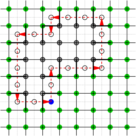
Figure 3: A worm moving through the dual lattice. The direct lattice is indicated by solid lines and the spins on the direct lattice by solid circles. The dual lattice is indicated by dashed lines and the sites on the dual lattice by open circles. As the worm moves through the lattice the bond-variables are flipped as indicated by the thick bonds in the figure.

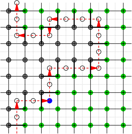
Figure 4: An illegal worm move. The worm winds around the lattice in the vertical direction and correspondingly all rows have an odd number of flipped bond-variables $b$. The direct lattice is indicated by solid lines and the spins on the direct lattice by solid circles. The dual lattice is indicated by dashed lines and the sites on the dual lattice by open circles. As the worm moves through the lattice the bond-variables are flipped as indicated by the thick bonds in the figure.

III.1 Algorithm C (Dual Worm Algorithm)

We now turn to a discussion of the dual algorithm. From the above description in terms of bond-variables it is now quite easy to define a geometrical worm algorithm on the dual lattice closely following previous work on such algorithms Alet and Sørensen (2003a, b). We denote the i’th site on the dual lattice that the worm visits as $d_{i}$. A “worm” is constructed by going through a sequence of neighboring sites on the dual lattice by each time choosing a direction $\sigma$ to follow according to an appropriately determined probability. When the worm moves from $d_{i}$ to $d_{i+1}$ the corresponding bond-variable $b_{i}$ that the worm crosses is flipped. The bond-variables can take on only 2 values $\pm 1$. Hence, the associated energy cost for flipping $b_{i}$ is given by $\Delta E=2J^{\alpha}_{j,k}b^{\alpha}(j,k),\ \alpha=x,y$. We can now define weights for each direction $\sigma$, $A^{E_{\sigma}}=\min(1,\exp(-\Delta E^{\sigma}/k_{B}T))$ used for determining the correct probability for choosing a new site. This is not the only choice for the weights. Other equivalent choices should work equally well. The bond-variables are updated during the construction of the worm and the worm is finished when the starting site on the dual site is reached again and the worm forms a closed loop. The dual worm algorithm can then be summarized using the following pseudo-code:

1. Choose a random initial site $d_{1}$ on the dual lattice.

2. For each of the directions $\sigma=\pm x,\pm y$ calculate the weights $A^{E_{\sigma}}$ associated with flipping the bond-variable perpendicular to that direction, $A^{E_{\sigma}}=\min(1,\exp(-\Delta E^{\sigma}/k_{B}T))$.

3. Calculate the normalization $N_{d_{i}}=\sum_{\sigma}A^{\sigma}$ and the associated probabilities $p^{\sigma}_{d_{i}}={A^{E_{\sigma}}}/{N_{d_{i}}}.$

4. According to the probabilities, $p^{\sigma}_{d_{i}}$, choose a direction $\sigma$.

5. Update the bond-variable $b^{\sigma}_{i}$ for the direction chosen and move the worm to the new dual lattice site $d_{i+1}$.

6. If $d_{i}\neq d_{1}$ goto 2.

7. Calculate the normalizations $\bar{N}_{d_{1}}$ and $N_{d_{1}}$ of the initial site, $s_{1}$, with and without the worm present. If the worm is “legal”, i.e. with even winding number in both the x- and the y-direction ($O^{x}_{w},\ O^{y}_{w}$ both 0 - see definition below), then erase the worm with probability $P_{e}=1-\min(1,N_{d_{1}}/{\bar{N}_{d_{1}}})$. If the worm is “illegal”, that is if either $O^{x}_{w}$ or $O^{y}_{w}$ calculated when the worm has closed equal 1, then always erase it. Goto 1

Following the above discussion of the boundary constraints it is easy determine if the winding number in the x- or y-direction is odd by simply choosing one row $k_{0}$ and one column $j_{0}$ and calculating the number of frustrated, $b=-1$, bond-variables:

$$O^{x} = \sum_{j}\frac{1-b^{x}(j,k_{0})}{2}\ ({\rm mod}2)$$

$$O^{y} = \sum_{k}\frac{1-b^{y}(j_{0},k)}{2}\ ({\rm mod}2),$$ (11)

since a worm with an odd winding number in the y-direction will result in $O^{x}$ being 1 independent of $k_{0}$, or equivalently for the x-direction and $O^{y}$. See Figure 4. $O^{x}$ and $O^{y}$ then takes on the values 1 or 0 depending on whether the corresponding winding numbers are odd or even.

Several points are noteworthy about this algorithm. To a great extent it is simply the dual version of the Wolff algorithm Wolff (1989). Each worm encloses a cluster of spins on the direct lattice (not necessarily a simply connected cluster). Flipping the bond-variables in the worm effectively flips the spin in the cluster. This correspondence is particular to two dimensions which is the only dimension where the present dual worm algorithm can be defined. The intuitive argument for this is that the bond-variables updated by the worm have to enclose a finite volume of spins on the direct lattice, this is only possible in two dimensions. In dimensions higher than two the one dimensional worms are not capable of enclosing a finite volume. Mathematically, it can be seen that the divergence less constraint, Eq. (7), cannot be satisfied under worm moves. Under most conditions the rejection probability, $P_{e}$, is very small, however, for small lattice sizes the probability for generating a worm with an odd winding number in either the x- or y-direction can be non-negligible. It is important to note that since the bond-variables are updated during the construction of the worm the generated configurations are not valid and the above constraints are not satisfied. However, once the construction of the worm is finished and the path of the worm closed, the divergenceless constraint is satisfied. Rejecting worms with odd winding numbers then assures that the resulting configurations are valid. Also, when the worm moves through the lattice it may pass many times through the same link and cross itself before it reaches the initial site where the construction terminates. Finally, at each step $i$ in the construction of the worm it is likely that the worm at the site $d_{i}$ will partially “erase” itself by choosing to go back to the site $d_{i-1}$ visited immediately before, thereby “bouncing” off the site $d_{i}$.

Proof of Algorithm C (Dual Worm Algorithm)

Now we turn to the proof of detailed balance for the algorithm. As before, let $\mu$ denote the configuration of the bond-variables without the worm, $w$, and $\nu$ the configuration with the worm. Let us consider the case where the worm, $w$, visits the sites $\{d_{1}\ldots d_{W}\}$ on the dual lattice. Here $d_{1}$ is the initial site. The worm then goes through the corresponding bond-variables $\{b_{1}\ldots b_{W}\}$. Note that, $d_{W}$ is the last site visited before the worm reaches $d_{1}$. Furthermore, let $E_{i}$ denote the energy required to flip the bond-variable $b_{i}$ from its position in the configuration $\mu$, with $-E_{i}$ the energy required to flip $b_{i}$ from its position in $\nu$ to that in $\mu$. The total probability for constructing the worm $w$ is then given by:

$$P(w;d_{1}\to d_{W})=$$

$$P(d_{1})(1-P_{e}(w))P({\rm legal}|w)\prod_{i=1}^{W}\frac{A^{E_{i}}}{{N_{d_{i}}}}.$$ (12)

The index $\sigma$ denotes the direction needed to go from $d_{i}$ to $d_{i+1}$, ($\pm x,\pm y$), crossing the bond-variable $b_{i}$. $P(d_{1})$ is the probability for choosing site $d_{1}$ as the starting point and $P_{e}(w)$ is the probability for erasing a “legal” worm after construction. Finally, $P({\rm legal}|w)$ is the conditional probability that the constructed worm $w$ is “legal”, with even winding numbers in both x- and y-directions. If the worm $w$ is legal and has been accepted we have to consider the probability for reversing the move. That is, we consider the probability for constructing an anti-worm $\bar{w}$ annihilating the worm $w$. Note that, in this case the sites are visited in the opposite order, $\bar{d}_{1}=d_{1},\bar{d}_{2}=d_{W},\ldots,\bar{d}_{W}=d_{2}$, in general $\bar{d}_{i}=d_{W-i+2}\ (i\neq 1)$. In the same manner the bond-variables are also visited in the reverse order $\bar{b}_{1}=b_{W},\bar{b}_{2}=b_{W-1},\ldots,\bar{b}_{W}=b_{1}$, in general $\bar{b}_{i}=d_{W-i+1}$.

Figure 5: The notation used for the proof of the dual worm algorithm. The configuration shown corresponds to a worm (solid line) partly erased by its corresponding anti-worm (dashed line).

Consequently, when describing $\bar{w}$, we directly use $d,b$ instead of $\bar{d},\bar{b}$. The notation is illustrated in Fig. 5. We therefore have:

$$P(\bar{w};\bar{d}_{1}\to\bar{d}_{W}) = P(d_{1})(1-P_{e}({\bar{w}}))P({\rm legal}|{\bar{w}})$$ (13)

$$\times \frac{A^{-E_{W}}}{{\bar{N}}_{d_{1}}}\prod_{i=W}^{2}\frac{A^{-E_{i-1}}}{{\bar{N}}_{d_{i}}}.$$

Please note that the index $i$ runs over $W,\ldots,2$. Let us now consider the case where both of the worms $w$ and $\bar{w}$ have reached the site $d_{i}$ different from the starting site $d_{1}$. See Fig. 5. Since we are updating the link variables during the construction of the worm we immediately see that $N_{d_{i}}=\bar{N}_{d_{i}}\ i\neq 1$. Furthermore, $A^{E_{i}}$ and $A^{-E_{i}}$ only depend on the bond-variable $b_{i}$, and we therefore see that:

$$\frac{A^{E_{i}}}{A^{-E_{i}}}=\exp(-\Delta E_{i}/k_{B}T),\ i=1\ldots W.$$ (14)

Hence, since $P(d_{1})$ is uniform through out the dual lattice, and since $w$ and $\bar{w}$ must wind the lattice in precisely the same manner resulting in $P({\rm legal}|w)=P({\rm legal}|{\bar{w}})$, we find:

$$\frac{P(w)}{P({\bar{w}})}=\frac{1-P_{e}({w})}{1-P_{e}({\bar{w}})}\frac{\bar{N}_{d_{1}}}{N_{d_{1}}}\exp(-\Delta E_{\rm Tot}/k_{B}T),$$ (15)

where $\Delta E_{\rm Tot}$ is the total energy difference between a configuration with and without the worm $w$ present. With our definition of $P_{e}$ we see that $(1-P_{e}(w))/(1-P_{e}(\bar{w}))=N_{d_{1}}/{\bar{N}_{d_{1}}}.$ Hence, with this choice of $P_{e}$ we satisfy detailed balance since:

$$\frac{P_{w}}{P_{\bar{w}}}=\exp(-\Delta E_{\rm Tot}/k_{B}T).$$ (16)

As was the case for the previous algorithms there are 2 ways of introducing a worm that will take us from $\mu\to\nu$, and equivalently 2 ways of introducing $\bar{w}$. (Strictly speaking, each of the two ways actually represents an infinite sum as discussed under the proof of algorithm A). In both cases Eq. (16) holds and it follows that $P(\mu\to\nu)=P(\nu\to\mu)\exp(-\Delta E_{\rm Tot}/k_{B}T)$ showing that detailed balance is satisfied. Ergodicity is simply proven as the worm can perform local loops and wind around the lattice in any direction. $\blacksquare$

Illegal worms: One should be cautious when treating “illegal” moves such as the worms with odd winding numbers encountered above. Suppose that our Monte Carlo algorithm has generated a number of configurations $C_{1},C_{2},C_{2},C_{3},\ldots,C_{i-1},C_{i}$ where some configurations are repeated since the worm moved has been rejected. From the configuration $C_{i}$ we now construct a worm that turns out to be “illegal” with odd winding numbers. From the above proof we then see that we have to repeat $C_{i}$ in the sequence of configurations since not repeating the configuration would lead to a total acceptance probability different from $(1-P_{e}(w))P({\rm legal}|w)$. For instance, imagine we kept generating worms till we found a “legal” one. This would make the total acceptance ratio a sum over the number of times we try which would be incorrect.

III.2 Algorithm D (Dual Directed Worm Algorithm)

Following the discussion of algorithm B it is straight forward to develop a directed version of algorithm C. As was the case for algorithm B we define conditional probabilities $p_{d_{i}}(m|n)$, corresponding to the probability for continuing in the direction $\sigma_{m}$ if the worm has come from direction $\sigma_{n}$. Since we in algorithm C, at each site on the dual lattice $d_{i}$, can go in four directions this leads us to define a $4\times 4$ matrix P at each site on the dual lattice. However, compared to algorithm B, the number of different matrices at a given dual site is now much smaller since the weights $A^{E_{i}}$ only depend on the associated bond-variable. In fact there are now only 16 possible matrices at a given site and these can easily be optimized and tabulated at the outset of the calculation. Even in the presence of disorder, a large number of them can be tabulated. This directed dual worm algorithm is now identical to algorithm C except for the fact that if $d_{i}$ is different from $d_{1}$, the $p_{d_{i}}^{\sigma}$ are selected from these optimized matrices (the same way at it was done for algorithm B). Due to the simplicity of this modification and the similarity with algorithm B, we do not present pseudo-code nor a proof for this directed algorithm. It is easy to see that rejection probability remains identical to the one used in algorithm C, $P_{e}(w)=1-\min(1,N_{d_{1}}/\bar{N}_{d_{1}})$.

III.3 Performance Algorithm C,D

In order to compare the two algorithms C and D defined on the dual lattice we have again calculated the autocorrelation function $C_{E}(t)$.

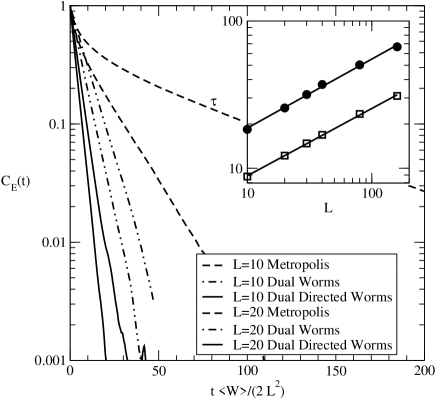
Figure 6: Autocorrelation functions for the energy $C_{E}(t)$ as a function of Monte Carlo time, calculated at $T_{c}$. Shown are results for $L=10,20$ for the Metropolis, dual worm and dual directed worm algorithms. Note that, in order to compare the 3 algorithms the time axis has been scaled so that in all cases 1 time step corresponds to an attempted update of all the variables. The inset shows the scaling of the autocorrelation time $\tau^{\prime}$ as a function of the system size for the dual worm and dual directed worm algorithm. The autocorrelation time is here rescaled: $\tau^{\prime}=\tau\langle$W$\rangle/(2L^{2})$. In both cases we find roughly a power-law form $\tau^{\prime}\simeq L^{0.46}$ shown as the solid lines in the inset. The autocorrelation functions shown were calculated averaging over 10-20 Million worms (MCS for the metropolis algorithm).

Table 1: Average worm size defined as the average number of bond-variables attempted to change during the construction of a any worm, including worms eventually rejected. Also listed is the estimated autocorrelation time, $\tau$, in units of worms constructed and the rescaled autocorrelation time $\tau^{\prime}=\tau\langle$W$\rangle/(2L^{2})$ in units of $2L^{2}$ attempted updates. The autocorrelation time is here here defined by $C_{e}(\tau)=0.05$. Results are listed for the dual and dual directed worm algorithms.

	Dual			Dual Directed
L	$\langle$W$\rangle$	$\tau$	$\tau^{\prime}$	$\langle$W$\rangle$	$\tau$	$\tau^{\prime}$
10	57	64.6	18.4	60	29.3	8.8
20	188	109.4	25.7	198	49.3	12.2
30	382	149.4	31.7	400	66.6	14.8
40	630	187.9	37.0	660	81.9	16.9
80	2119	303.8	50.3	2204	135.9	23.4
160	7132	478.8	66.7	7408	214.3	31.0

Our results are shown in Fig. 6 and tabulated in Table 1. As on the direct lattice we use the energy to calculate the autocorrelation functions. For algorithms C and D we have constructed 10 million worms for the smaller lattices and 20 million for the largest lattice (L=160). We compare to the Metropolis algorithm where each time step corresponds to an attempted update of the $L^{2}$ spins. Since the worm algorithm in this case on average only attempts to update $\langle W\rangle$ out of the $2L^{2}$ bond-variables we have to rescale the time-axis by a factor of $\langle W\rangle/(2L^{2})$ when we compare algorithms C and D to the Metropolis algorithm. We can therefore define an autocorrelation time $\tau$ in units of worms constructed and a rescaled autocorrelation time $\tau^{\prime}=\tau\langle W\rangle/(2L^{2})$ in units of $2L^{2}$ attempted updates. In order to simplify the analysis of the data we define the autocorrelation time as $C_{E}(\tau)\equiv 0.05$. As can be seen in Fig. 6 the dual worm algorithms represents a dramatic improvement over the Metropolis algorithm. We have not plotted results for the Swendsen-Wang algorithm on the direct lattice since for $L=10$ they are indistinguishable from the results obtained for the dual directed worm algorithm. The scaling of $\tau^{\prime}$ with $L$ is a relatively small power-law $\tau^{\prime}\sim L^{0.46}$. This exponent is small but larger than most values quoted for the Swendsen-Wang and Wolff algorithms. This is perhaps not too surprising since the worms are allowed to cross themselves thereby erasing previous updates. The difference in autocorrelation times between algorithm C and its directed version D appears to be a constant factor. Therefore, the direction of algorithm C does not change the exponent $z_{MC}$.

For a $10\times 10$ lattice at $T_{c}$ roughly 85% of all constructed worms are accepted and about 10% of the constructed worms are “illegal” when simulations are performed using the dual geometric worm algorithm. For the directed version of the algorithm the corresponding numbers are 75% and 20%. The number of illegal worms drops rapidly with $L$ and for $L=30$ 90% of the worms are accepted with 5% illegal worms for the undirected algorithm compared to 83% and 10% for the directed dual algorithm.

The presented dual algorithms are quite general since they depend only in a relatively limited way on the underlying Hamiltonian. Even though they may not be competitive with the Swendsen-Wang and Wolff algorithms for the Ising model they may be quite interesting to apply to other two-dimensional models that can be formulated in terms of bond-variables and where more effective cluster algorithms are difficult to define.

III.4 Domain Wall Free Energy

A quantity of particular interest in many studies of ordering transitions is the domain wall free energy, the difference in free energy between configurations of the system with periodic (P) and anti-periodic (AP) boundary conditions in one direction, $\Delta F=F_{\rm AP}-F_{\rm P}$. The domain wall free energy can be shown to obey simple scaling relations and is a very efficient tool for distinguishing between different ordered phases. Unfortunately, it is usually very difficult to calculate free energies directly in Monte Carlo simulations. A clever trick to do so is the boundary flip MC method, proposed by Hasenbusch Hasenbusch (1993); Hukushima (1999), where the coupling constants at the boundary are considered as dynamical variables, and can be flipped during the course of the MC simulation. If $P_{P}(T)$ and $P_{A}P(T)$ describe the probability to obtain MC configurations with periodic and anti-periodic boundary conditions and and $Z_{\rm P},Z_{\rm AP}$ the associated partition functions, then the domain wall free-energy is given by:

$$e^{-\beta(F_{\rm AP}-F_{\rm P})}=\frac{Z_{\rm AP}}{Z_{\rm P}}=\frac{P_{\rm AP}(T)}{P_{\rm P}(T)}.$$ (17)

Effectively, the boundary flip MC method attempts to sample the ratio $Z_{\rm AP}/Z_{\rm P}$, and this is usually cumbersome. However, for the dual algorithms it is trivial to obtain this ratio. It follows from Eq. (9), that if we allow the constructed worms to have all different kinds of winding around the torus (making all worms legal) then we are sampling a partition function which is a sum of four terms:

$$Z=Z_{\rm P_{x},P_{y}}+Z_{\rm AP_{x},P_{y}}+Z_{\rm P_{x},AP_{y}}+Z_{\rm AP_{x},AP_{y}}$$ (18)

Here, $Z_{\rm BC_{x},BC_{y}}$ is the partition function with BC_x(BC_y) in the x(y)-direction. This is so, because we can turn an illegal worm into a legal worm by changing the boundary condition in the direction(s) where the winding of the worm violates Eq. (9). During the MC simulation it is easy to see to which term a given configuration contributes simply by keeping track of the total winding number in both the x- and y-direction. See eq. (11). When this is even, the boundary condition in the associated direction is periodic, and if it is odd the boundary condition is anti-periodic. In order to calculate $Z_{\rm AP_{x},P_{y}}/Z_{\rm P_{x},P_{y}}$ we therefore simply have to count how many times the total winding number is odd in the x-direction and even in the y-direction and divide with the number of times it is even in both direction. Due to its simplicity, we expect this approach to be an extremely efficient way of calculating $\Delta F$. In table 2 we show preliminary results for $\Delta F/kT$ calculated with $10^{8}$ worms for the two-dimensional Ising model at $T_{c}$. For reference we compare to exact results obtained using pfaffians Sørensen (2000).

We are grateful to Philippe de Forcrand for suggesting the above way of calculating $\Delta F$.

Table 2: The domain wall free-energy $\Delta F/kT$ for several system sizes calculated at the critical temperature $T_{c}$ obtained using our MC method and exact results from Ref. Sørensen, 2000.

L	Exact	MC
4	0.9658246670	0.9654(5)
16	0.9853282229	0.985(10)
24	0.9859725679	0.985(10)
32	0.9861972559	0.986(10)
48	0.9863574947	0.986(10)
64	0.9864135295	0.984(20)

IV Discussion

We have presented two generalizations of the geometrical worm algorithm applicable to classical statistical mechanics model. The first algorithm exploits linear worms on the direct lattice, the other closed loops of worms on the dual lattice. In both cases have we developed directed versions of the algorithms. While the first algorithm is applicable in any spatial dimension, it is quite clear that for topological reasons it is only possible to define a worm algorithm of the proposed kind on the dual lattice in two spatial dimensions.

Due to its poor performance the linear worm algorithm (A) is mainly of interest from the perspective of fostering the development of new and more advanced algorithms. The linear worm algorithm presents a number of very attractive features such as the possibility to choose the distribution of the worm lengths and it seems possible to significantly improve the performance of the algorithm (and most other geometrical worm algorithms) by eliminating the rejection probability. So far, we have been unable to do so, but this would clearly be very interesting since the algorithms then would be quite promising for the study of frustrated or even disordered models where other cluster algorithms fail.

The dual worm algorithm is very efficient and even though the obtained $z_{MC}$ is larger than for the Swendsen-Wang algorithm it is quite competitive since it requires relatively little overhead and is very simple to implement. One of the most interesting features of this algorithm is the topological aspect of the worms, resulting in forbidden worm moves.

The geometrical worm algorithm has in some cases been very successfully applied to the study of models with disorder Alet and Sørensen (2003a). We therefore applied both the linear and dual worm algorithm to the bond disordered Ising model. In both cases do the algorithms perform worse than the Metropolis algorithm. For the dual worm algorithm this failure is due to the fact that the average size of worms diverge when glassy phases are approached. The linear worm algorithm would seem more promising for study of models with disorder since the length of the worms can be controlled from the outset. In fact the performance of the algorithm is in this case quite comparable to the Metropolis algorithm (which has a diverging $\tau$ close to a glassy phase). One might have expected the linear worm algorithm to perform significantly better than the Metropolis algorithm when disorder is present. We assume that the fact that it is only comparable to the Metropolis algorithm is because large parts of the spins are not effectively flipped since worms are mostly rejected in those parts of the lattice. If this is true, a modified version of the linear worm algorithm with $P_{e}\equiv 0$ or with a much more ingenious choice of the neighbors would be of considerable interest since it would hold the potential to sample such disordered models significantly more effectively than the Metropolis algorithm.

Appendix A Proof of Algorithm A

The probability for creating the worm, $w$, starting from site $s_{1}$ is given by:

$$P(w;s_{1}\to s_{W})= P(W)P(s_{1})\frac{A^{E_{2}}_{s_{2}}}{N_{s_{1}}}\frac{A^{E_{3}}_{s_{3}}}{N_{s_{2}}}\ldots$$ (19)

$$\times\frac{A^{E_{W}}_{s_{W}}}{N_{s_{W-1}}}(1-P_{e}(w))$$

Here $P(W)$ denotes the probability for choosing a worm length of $W$. The probability for introducing an anti-worm, $\bar{w}$, starting at the site $s_{1}$, erasing the worm by going in the opposite direction along $w$ becomes:

$$P(\bar{w};s_{W}\to s_{1})= P(W)P(s_{W})\frac{A^{-E_{W-1}}_{s_{W-1}}}{\bar{N}_{s_{W}}}\ldots$$ (20)

$$\times\frac{A^{-E_{2}}_{s_{2}}}{\bar{N}_{s_{3}}}\frac{A^{-E_{1}}_{s_{1}}}{\bar{N}_{s_{2}}}(1-P_{e}(\bar{w}))$$

Since neither $N_{s_{i}}$ nor $\bar{N}_{s_{i}}$ depend on the position of the spin on the site $i$ and since the spins are visited in the precise opposite order for the anti-worm with respect to the worm, we then see that $N_{s_{i}}=\bar{N}_{s_{i}}$ $\forall i\neq 1,W$, and we find:

$$\frac{P(w;s_{1}\to s_{W})}{P(\bar{w};s_{W}\to s_{1})}=\frac{1-P_{e}(w)}{1-P_{e}(\bar{w})}\frac{A^{E_{2}}_{s_{2}}\ldots A^{E_{W}}_{s_{W}}}{A^{-E_{W-1}}_{s_{W-1}}\ldots A^{-E_{1}}_{s_{1}}}\frac{\bar{N}_{s_{w}}}{N_{s_{1}}}$$ (21)

Since $A^{E_{i}}_{s_{i}}/A^{-E_{i}}_{s_{i}}=\exp(-\Delta E_{i}/k_{B}T)$ we see, using our definition of $P_{e}$, that

$$\frac{P(w;s_{1}\to s_{W})}{P(\bar{w};s_{W}\to s_{1})}=\exp(-\Delta E/k_{B}T).$$ (22)

Quite generally, there is more than one way to introduce a worm to go from $\mu$ to $\nu$. In fact there are 2 ways of introducing a worm taking the system from configuration $\mu$ to $\nu$, one where the worm traverses the sites from $s_{1}$ to $s_{W}$ and another where the worm traverses the sites from $s_{W}$ to $s_{1}$. Equivalently, there are 2 ways of introducing the anti-worm. Hence, $P(\mu\to\nu)$ is a sum of the two probabilities, $P(\mu\to\nu)=P(w;s_{1}\to s_{W})+P(w;s_{W}\to s_{1})$. However, employing the result we have just proven we see that:

$$P(\mu\to\nu)= \left[P(\bar{w};s_{W}\to s_{1})+P(\bar{w};s_{1}\to s_{W})\right]$$

$$\times\exp(-\Delta E/k_{B}T)$$

$$= P(\nu\to\mu)\exp(-\Delta E/k_{B}T).$$ (23)

Hence, the proposed algorithm satisfies detailed balance on a bi-partite lattice and we see that detailed balance is satisfied no matter how many possible ways one can introduce a worm in order to go from $\mu\to\nu$ as long as the number of possible anti-worms matches. Strictly speaking, since the worm can partly erase itself, there is in fact an infinite number of worm-moves that will take us from $\mu$ to $\nu$, however, in each case there is a matching anti-worm so we can replace the above sum over two probabilities with an infinite sum, yielding the same conclusion. Ergodicity is proven by noting that single spin flips are incorporated in the algorithm. $\blacksquare$

Appendix B Proof of Algorithm B

The proof is quite similar to the proof of algorithm A and we use the same notation. The probability for creating a worm, $w$, starting from site $s_{1}$ is then given by:

$$P(w;s_{1}\to s_{W})=P(W)P(s_{1})\frac{A^{E_{2}}_{s_{2}}}{N_{s_{1}}}p_{s_{2}}(s_{3}|s_{1})\ldots\ldots$$

$$p_{s_{W-2}}(s_{W-1}|s_{W-3})p_{s_{W-1}}(s_{W}|s_{W-2}).(1-P_{e}(w))$$ (24)

Here $P(s_{1})$ denotes the probability for choosing site $s_{1}$ as the starting site for the worm, $P(W)$ the probability for choosing a worm length $W$. $p_{s_{i}}(s_{i+1}|s_{i-1})$ denotes the conditional probability, extracted from the minimized matrix $P$, at the site $s_{i}$ for continuing to the site $s_{i+1}$ knowing that the worm is coming from the site $s_{i-1}$. Starting from the configuration $\nu$ we can now calculate the probability for introducing an anti-worm, $\bar{w}$, starting at the site $s_{W}$, erasing the worm, $w$. We find:

$$P(\bar{w}; s_{W}\to s_{1} )=P(W)P(s_{W})\frac{A^{-E_{W-1}}_{s_{W-1}}}{\bar{N}_{s_{W}}}\bar{p}_{s_{W-1}}(s_{W-2}|s_{W})$$ (25)

$$\ldots \bar{p}_{s_{3}}(s_{2}|s_{4})\bar{p}_{s_{2}}(s_{1}|s_{3})(1-P_{e}(\bar{w})).$$

At a given site, $s_{i}$, the configurations of the spins during the construction of the worm and the anti-worm only differ by the position of the spin at the site itself. Since the set of neighbors $\sigma$ exclude any nearest neighbors to $s_{i}$ we see that $P_{s_{i}}=\bar{P}_{s_{i}}$. Hence, by construction,

$$\frac{p_{s_{i}}(s_{i+1}|s_{i-1})}{\bar{p}_{s_{i}}(s_{i-1}|s_{i+1})}=\frac{A_{s_{i+1}}^{E_{i+1}}}{A^{-E_{i-1}}_{s_{i-1}}}.$$ (26)

Using the definition of $P_{e}$ and the fact that $P(s_{1})=P(s_{W})$, we then see that:

$$\frac{P(w;s_{1}\to s_{W})}{P(\bar{w};s_{W}\to s_{1})}=\frac{A^{E_{1}}_{s_{1}}\ldots A^{E_{W}}_{s_{W}}}{A^{-E_{1}}_{s_{1}}\ldots A^{-E_{W}}_{s_{W}}}.$$ (27)

Since $A^{E_{i}}_{s_{i}}/A^{-E_{i}}_{s_{i}}=\exp(-\Delta E_{i}/k_{B}T)$ we finally see that

$$\frac{P(w;s_{1}\to s_{W})}{P(\bar{w};s_{W}\to s_{1})}=\exp(-\Delta E/k_{B}T),$$ (28)

where $\Delta E$ is the total energy cost in going from configuration $\mu$ to configuration $\nu$. As was the case for algorithm A, there are 2 ways of introducing a worm taking the system from configuration $\mu$ to $\nu$ (modulo sites visited an even number of times), one where the worm traverses the sites from $s_{1}$ to $s_{W}$ and another where the worm traverses the sites from $s_{W}$ to $s_{1}$. Equivalently, there are 2 ways of introducing the anti-worm. We again see that detailed balance is satisfied. Ergodicity is proven by noting that single spin flips are incorporated in the algorithm, since for $W=1$ the algorithm corresponds to attempting a Metropolis spin-flip at the selected site.$\blacksquare$

References

- Prokof’ev and Svistunov (2001) N. Prokof’ev and B. Svistunov, Phys. Rev. Lett 87, 160601 (2001).
- Swendsen and Wang (1987) R. H. Swendsen and J. S. Wang, Phys. Rev. Lett. 58, 86 (1987).
- Wolff (1989) U. Wolff, Phys. Rev. Lett. 62, 361 (1989).
- Machta et al. (1995) J. Machta, Y. S. Choi, A. Lucke, T. Schweizer, and L. V. Chayes, Phys. Rev. Lett 75, 2792 (1995).
- Wang and Landau (2001) F. Wang and D. P. Landau, Phys. Rev. Lett. 86, 2050 (2001).
- Prokof’ev et al. (1998) N. V. Prokof’ev, B. V. Svistunov, and I. S. Tupitsyn, Phys. Lett. A 238, 253 (1998).
- Alet and Sørensen (2003a) F. Alet and E. S. Sørensen, Phys. Rev. E 67, R015701 (2003a).
- Alet and Sørensen (2003b) F. Alet and E. S. Sørensen, Phys. Rev. E 68, 026702 (2003b).
- Newman and Barkema (1999) M. E. J. Newman and G. T. Barkema, Monte Carlo Methods in Statistical Physics (Oxford University Press, 1999).
- Landau and Binder (2000) D. P. Landau and K. Binder, A Guide to Monte Carlo Methods in Statistical Physics (Cambridge University Press, 2000).
- Syljuåsen and Sandvik (2002) O. F. Syljuåsen and A. W. Sandvik, Phys. Rev. E 66, 046701 (2002).
- Barkema and Marko (1993) G. T. Barkema and J. F. Marko, Phys. Rev. Lett. 71, 2070 (1993).
- Newman and Barkema (1996) M. E. J. Newman and G. T. Barkema, Phys. Rev. E 53, 393 (1996).
- Kadanoff (2000) L. P. Kadanoff, Statistical Physics, Statics, Dynamics and Renormalization (World Scientific, 2000).
- Hasenbusch (1993) M. Hasenbusch, J. Phys. I 3, 753 (1993).
- Hukushima (1999) K. Hukushima, Phys. Rev. E 60, 3606 (1999).
- Sørensen (2000) E. Sørensen, cond-mat/0006233 (2000).