Superconducting qubit storage and entanglement with nanomechanical resonators

Abstract

We describe a quantum computational architecture based on integrating nanomechanical resonators with Josephson junction phase qubits, with which we implement single- and multi-qubit operations. The nanomechanical resonator is a GHz-frequency, high-quality-factor dilatational resonator, coupled to the Josephson phase through a piezoelectric interaction. This system is analogous to one or more few-level atoms (the Josephson qubits) in a tunable electromagnetic cavity (the nanomechanical resonator). Our architecture combines the best features of solid-state and cavity-QED approaches, and may make possible multi-qubit processing in a scalable, solid-state environment.

The lack of scalable qubit architectures, with sufficiently long quantum-coherence lifetimes and a suitably controllable entanglement scheme, remains the principal roadblock to building a large-scale quantum computer. Superconducting devices exhibit robust macroscopic quantum behavior Makhlin et al. (2001). Recently, there have been exciting demonstrations of long-lived Rabi oscillations in current-biased Josephson junctions Yu et al. (2002); Martinis et al. (2002), subsequently combined with a two-qubit coupling scheme Berkley et al. (1998), and in parallel, demonstrations of Rabi oscillations and Ramsey fringes in a Cooper-pair box Nakamura et al. (1999, 2002); Vion et al. (2002). These accomplishments have generated significant interest in the potential for Josephson-junction-based quantum computation Leggett (2002). Coherence times $\tau_{\rm\varphi}$ up to 5$\,\mu$s have been reported in the current-biased devices Yu et al. (2002), with corresponding quality factors $Q_{\rm\varphi}\equiv\tau_{\rm\varphi}\,\Delta E/h$ of the order of $10^{5}$, yielding sufficient coherence to perform many logical operations. Here $\Delta E$ is the qubit energy level spacing.

In this paper, we describe an architecture in which ultrahigh-frequency resonators coherently couple two or more current-biased Josephson junctions, where the superconducting “phase qubits” are formed from the energy eigenstates of the junctions. We show that the system is analogous to one or more few-level atoms (the Josephson junctions) in a tunable electromagnetic cavity (the resonator), except that here we can individually tune the energy level spacing of each atom, and control the electromagnetic interaction strength.

Other investigators have proposed the use of electromagnetic Shnirman et al. (1997); Makhlin et al. (1999); Mooij et al. (1999); Makhlin et al. (2000); You et al. (2002); Plastina and Falci (2003); Blais et al. (2003); Smirnov and Zagoskin or superconducting Buisson and Hekking (2001); Marquardt and Bruder (2001) resonators to couple Josephson junctions together. The use of nanomechanical resonators to mediate multi-qubit operations has not to our knowledge been described previously, although an approach to create entangled states of a single resonator has been proposed Armour et al. (2002). The use of mechanical as opposed to electromagnetic resonators has the advantage that potentially much higher quality factors can be achieved Yang et al. (2000), with significantly smaller dimensions, enabling a truly scalable approach.

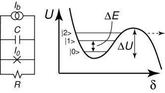
Figure 1: Left: Equivalent-circuit model for a current-biased Josephson junction. A capacitance $C$ and resistance $R$ in parallel with an ideal Josephson element with critical current $I_{0}$, all with a bias current $I_{b}$. Right: Metastable potential well in the cubic potential limit, showing the barrier height $\Delta U$ that separates the metastable states from the continuum. Here there are three quasi-bound states $|0\rangle$, $|1\rangle$, and $|2\rangle$, the lower two separated in energy by $\Delta E$.

Our implementation uses large-area current-biased Josephson junctions, with capacitance $C$ and critical current $I_{0}$; a circuit model is shown in Fig. 1. The largest relevant energy is the Josephson energy $E_{\rm J}\equiv\hbar I_{0}/2e$, with a charging energy $E_{\rm c}\equiv(2e)^{2}/2C\ll E_{\rm J}$. The dynamics of the Josephson phase difference $\delta$ is that of a particle of mass $M=\hbar^{2}C/4e^{2}$ moving in an effective potential $U(\delta)\equiv-E_{\rm J}(\cos\delta+s\,\delta)$, for bias current $s=I_{\rm b}/I_{0}$ Barone and Paterno (1982); Fulton and Dunkleberger (1974). For bias currents $s<1$, the potential $U(\delta)$ has metastable minima, separated from the continuum by a barrier $\Delta U\equiv U(\delta_{\rm max})-U(\delta_{\rm min})\rightarrow(4\sqrt{2}/3)E_{\rm J}(1-s)^{3/2}$ for $s\rightarrow 1^{-}$, as shown in Fig. 1. The curvature $U^{\prime\prime}(\delta)$ defines the small-amplitude plasma frequency $\omega_{\rm p}\equiv\sqrt{U^{\prime\prime}(\delta_{\rm min})/M}=\omega_{{\rm p}0}(1-s^{2})^{1/4}$, with $\omega_{{\rm p}0}=\sqrt{2eI_{0}/\hbar C}=\sqrt{2E_{\rm c}E_{\rm J}}/\hbar$. The Hamiltonian for the junction phase difference is $H_{\rm J}=P^{2}/2M+U(\delta)$, with $P=-i\hbar d/d\delta$ the momentum operator. The junction’s zero-voltage state corresponds to the phase “particle” trapped in one of the metastable minima.

The lowest two quasi-bound states in a local minimum, $|0\rangle$ and $|1\rangle$, define the phase qubit. State preparation is typically carried out with $s$ just below unity, in the range $s=0.95-0.99$, where $U(\delta)$ is strongly anharmonic, and for which there are only a few quasibound states Martinis et al. (2002); Berkley et al. (1998). The anharmonicity allows state preparation from a classical radiofrequency (rf) field, as then the frequency of the classical field can be set to couple to only the lowest two states. In our scheme, by contrast, single quanta are exchanged between the junction and the resonator, so anharmonicity is not necessary; we find it convenient to work with $s$ between 0.5 and 0.9.

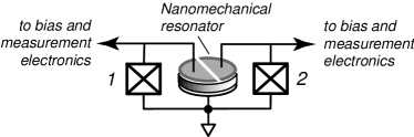
Figure 2: Proposed architecture for two-qubit entanglement. The qubits are the two Josephson junctions, coupled to a resonator, shown as a disc with a split gate.

We focus here on coupling a single resonator to two Josephson qubits; extensions to larger systems will be considered in later work. The two-junction circuit is shown in Fig. 2. The disk-shaped element is the nanomechanical resonator, consisting of a single-crystal piezoelectric disc sandwiched between two metal plates, and the junctions are the crossed boxes on either side of the resonator, interrogated by high-impedance circuits Martinis et al. (2002).

The phase qubit state $|0\rangle$ of a single junction is prepared by waiting for any excited component to decay. The pure state $|1\rangle$, or a superposition state $\alpha|0\rangle+\beta|1\rangle$, is prepared by adding a classical rf current $I_{\rm rf}$ to the bias, $I_{\phi 1}(t)=I_{\rm dc}+I_{\rm rf}^{\rm c}\cos(\omega_{\rm rf}t)+I_{\rm rf}^{\rm s}\sin(\omega_{\rm rf}t)$. Both $I_{\rm dc}$ and $I_{\rm rf}^{\rm s,c}$ vary slowly compared to $\hbar/\Delta E$. When $\omega_{\rm rf}$ is near resonance with the level spacing $\Delta E/\hbar$, the qubit will undergo Rabi oscillations, allowing the controlled preparation of linear combinations of $|0\rangle$ and $|1\rangle$.

The nanomechanical resonator is designed with a fundamental thickness resonance frequency $\omega_{0}/2\pi\sim 1-10\,{\rm GHz}$, with quality factor $Q\sim 10^{5}-10^{6}$. Piezoelectric dilatational resonators with resonance frequencies in this range, and quality factors of $10^{3}$ at room temperature, have been fabricated from sputtered AlN Ruby and Merchant (1994); Ruby et al. (2001). Single-crystal AlN can also be grown by chemical vapor deposition Cleland et al. (2001). Our simulations are based on such a resonator, with a diameter $d=1.16~{}\mu$m and thickness $b=0.5~{}\mu m$ pie . Such resonators can be used to coherently store a qubit state prepared in a current-biased Josephson junction, return it to that junction, or transfer it to another junction, as well as entangle two or more junctions. These operations are performed by tuning the energy level spacing $\Delta E$ into resonance with $\hbar\omega_{0}$, generating electromechanical Rabi oscillations.

Referring to Fig. 2, the total bias current of junction 1 is $I_{\rm dc1}+I_{\rm res}$, where $I_{\rm res}$ is the current through the resonator from that junction. A simple model for the resonator allows us to write $I_{\rm res}=C_{\rm res}(\dot{V}+h_{33}b\dot{U})$, where $C_{\rm res}$ is the resonator geometric capacitance, $h_{33}$ the relevant piezoelectric coupling constant Auld (1990), $\dot{V}$ the rate of voltage change, and $\dot{U}$ the rate of change of the mechanical strain. The current $I_{\rm res}$ is partly due to the capacitance $C_{\rm res}$ and partly due to the piezoelectrically-coupled strain $U$. $C_{\rm res}$, in parallel with the junction capacitance $C$, renormalizes the mass $M$ to $\tilde{M}=\hbar^{2}\tilde{C}/4e^{2}$, where $\tilde{C}=C+C_{\rm res}$.

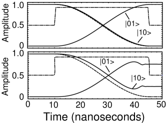
Figure 3: (a) Phase qubit storage. Solid curves are for $|c_{10}(t)|^{2}$ and $|c_{01}(t)|^{2}$, dashed curve is analytic RWA for $|c_{10}(t)|^{2}$, dash-dotted curve is $s(t)$. (b) Qubit storage with arctangent bias-current profile. All other parameters are the same as in (a). Solid curves are numerical results for $|c_{10}(t)|^{2}\!$ and $|c_{01}(t)|^{2}$.

With the resonator coupled to the superconducting phase through the voltage $V$, the Hamiltonian for the combined junction-resonator system is $H=H_{\rm J}+H_{\rm res}+\delta H$. Here $H_{\rm res}=\hbar\omega_{0}a^{\dagger}a$ is the Hamiltonian of the isolated resonator, where we have quantized the resonator displacement field with creation (destruction) operators $a^{\dagger}$ ($a$), and only included the fundamental dilatational mode. $\delta H$ is the phase-resonator interaction,

$$\delta H=\frac{\hbar C_{\rm res}bh_{33}}{2e(1-\eta)}\delta{\dot{U}}\,\delta=ig(a-a^{\dagger})\delta,$$ (1)

where $\eta=0.054$ and the coupling constant $g$ is

$$g=\frac{\hbar^{3/2}\,C_{\rm res}h_{33}\,\sqrt{\omega_{0}}}{(1-\eta)e\,\sqrt{\rho\pi bd^{2}/4}}.$$ (2)

For our model resonator $g\approx 0.820~{}\mu$eV.

Table 1: Final state amplitudes $c_{mn}(\pi/\Omega_{\rm d})$ for phase-qubit coupled to nanomechanical resonator.

probability amplitude	${\rm Re}\,c_{mn}$	${\rm Im}\,c_{mn}$	$|c_{mn}|^{2}$
$c_{00}$	$0.010$	$-0.003$	$0.000$
$c_{01}$	$-0.257$	$-0.966$	$1.000$
$c_{10}$	$0.009$	$0.041$	$0.002$
$c_{11}$	$-0.010$	$0.003$	$0.000$

In the junction eigenstate basis, the junction Hamiltonian is $H_{\rm J}=\sum_{m}\epsilon_{m}c_{m}^{\dagger}c_{m}$, with creation (destruction) operators $c_{m}^{\dagger}$ ($c_{m}$) acting on the phase qubit states. The interaction Hamiltonian is

$$\delta H=ig\sum_{mm^{\prime}}\langle m|\delta|m^{\prime}\rangle\,c_{m}^{\dagger}c_{m^{\prime}}(a-a^{\dagger}).$$ (3)

The eigenstates of the noninteracting Hamiltonian $H_{0}=H_{\rm J}+H_{\rm res}$ are $|mn\rangle\equiv|m\rangle_{\rm J}\otimes|n\rangle_{\rm res}$, with energies $E_{mn}=\epsilon_{m}+\hbar\omega_{0}\,n$, where $n$ is the resonator occupation number. An arbitrary state can be expanded as $|\Psi(t)\rangle=\sum_{mn}c_{mn}(t)|mn\rangle\exp(-iE_{mn}t/\hbar)$.

The full Hamiltonian is equivalent to a few-level atom in an electromagnetic cavity. The cavity “photons” are phonons, which interact with the “atoms” (here the Josephson junctions) via the piezoelectric effect. This analogy allows us to adapt quantum-information protocols developed for cavity-QED to our architecture.

Figure 4: Qubit transfer between two junctions. Solid curve is $|c_{100}(t)|^{2}\!$, dashed-dotted curve is $|c_{001}(t)|^{2}\!$, dashed curve is $|c_{010}(t)|^{2}\!$. Thin solid and dotted curves show $s_{1}(t)$ and $s_{2}(t)$.

We first show that we can coherently transfer a qubit state from a junction to a resonator, using the adiabatic approximation combined with the rotating-wave approximation (RWA) of quantum optics Scully and Zubairy (1997). We assume that the bias current $s$ changes slowly on the time scale $\hbar/\Delta E$, and work at temperature $T=0$. The RWA is valid when $\Delta E$ and $\hbar\omega_{0}$ are close on the scale of $\hbar\omega_{0}/Q_{\rm res}$, and when the interaction strength $g\ll\Delta E$. At time $t=0$, we prepare the resonator in the state $|0\rangle_{\rm res}$. In the RWA, neglecting relaxation, we obtain the amplitude evolution

$$i\hbar\,\partial_{t}c_{0n} = -ig\,\sqrt{n}\ \langle 0|\delta|1\rangle\,e^{i\omega_{\rm d}t}\,c_{1,n-1}$$

$$i\hbar\,\partial_{t}c_{1n} = ig\,\sqrt{n+1}\ \langle 1|\delta|0\rangle\,e^{-i\omega_{\rm d}t}\,c_{0,n+1},$$ (4)

where $\omega_{\rm d}\equiv\omega_{0}-\Delta E/\hbar$ is the resonator–qubit detuning. We integrate to find the reduced density matrices $\rho_{\rm J}(t)$ (in the qubit subspace) and $\rho_{\rm res}(t)$ (in the zero- and one-phonon resonator subspace). The junction phase is initially prepared in the pure state $\alpha|0\rangle_{\rm J}+\beta|1\rangle_{\rm J}$, corresponding to the reduced density matrix

$$\rho_{\rm J}(0)=\begin{bmatrix}|\alpha|^{2}&\alpha\beta^{*}\\ \alpha^{*}\beta&|\beta|^{2}\end{bmatrix}.$$ (5)

We allow the junction and resonator to interact on resonance for a time $\Delta t=\pi/\Omega_{d}$, where the Rabi frequency is $\Omega_{d}=(\Omega_{0}^{2}+\omega_{\rm d}^{2})^{1/2}$, in terms of the tuned (resonant) value $\Omega_{0}=2g|\langle 0|\delta|1\rangle|/\hbar$. After the interval $\Delta t$, the resonator is found to be in the same pure state,

$$\rho_{\rm res}(\pi/\Omega_{d})=\begin{bmatrix}|\alpha|^{2}&-\alpha\beta^{*}e^{i\pi\omega_{0}/\Omega_{d}}\\ -\alpha^{*}\!\beta\,e^{-i\pi\omega_{0}/\Omega_{d}}&|\beta|^{2}\end{bmatrix},$$ (6)

apart from expected phase factors. The phase qubit state has been swapped with that of the resonator. The cavity-QED analog of this operation has been demonstrated experimentally in Ref. Maître et al. (1997).

Table 2: Final amplitudes $c_{m_{1}m_{2}n}$ for state transfer.

probability amplitude	${\rm Re}\,c_{m_{1}m_{2}n}$	${\rm Im}\,c_{m_{1}m_{2}n}$	$|c_{m_{1}m_{2}n}|^{2}$
$c_{100}$	$0.038$	$-0.013$	$0.002$
$c_{001}$	$-0.314$	$0.152$	$0.121$
$c_{010}$	$-0.882$	$0.422$	$0.956$

To assess the limitations of the RWA, we also numerically integrated the exact amplitude equations

$$i\hbar\,{\dot{c}}_{mn}=\sum_{m^{\prime}n^{\prime}}\langle mn|\delta H|m^{\prime}n^{\prime}\rangle e^{i(E_{mn}-E_{m^{\prime}n^{\prime}})t/\hbar}\,c_{m^{\prime}n^{\prime}}.$$ (7)

The Josephson junction had parameters corresponding Ref. Martinis et al. (2002), $E_{\rm J}=43.05\,{\rm meV}$ and $E_{\rm c}=53.33\,{\rm neV}$. We used a 4th-order Runge-Kutta method with a time step of $10\,{\rm fs}$. Our main result is shown in Fig. 3. The qubit transfer depends sensitively on the shape of the profile $s(t)$, which starts at $s=0.50$, and is then adiabatically changed to the resonant value $s=0.928$. We find that the time during which $s$ changes should be at least exponentially localized. This can be understood by recalling that the RWA requires the qubit to be exactly in resonance with the resonator (in the $Q\rightarrow\infty$ limit). Therefore one must bring the system into resonance as quickly as possible without violating adiabaticity. The power-law tails associated with an arctangent function, for example, lead to large deviations from the desired behavior, shown in Fig. 3(b). The result in Fig. 3(a) was obtained using trapezoidal profiles with a cross-over time of $0.5\,{\rm ns}$. All quasibound junction states were included in the calculation, and convergence with the resonator’s Hilbert space dimension was obtained. The junction is held in resonance for half a Rabi period $\pi/\Omega_{d}$, during which energy is exchanged at the Rabi frequency. The systems are then brought out of resonance. The final state amplitudes are given in Table 1, and are quite close to the RWA results.

To pass a qubit state $\alpha|0\rangle+\beta|1\rangle$ from junction 1 to junction 2, the state is loaded into the first junction and the bias current changed to bring the junction into resonance with the resonator for half a Rabi period. This writes the state $\alpha|0\rangle+\beta|1\rangle$ into the resonator. After the first junction is taken out of resonance, the second junction is brought into resonance for half a Rabi period, passing the state to the second junction. We have simulated this operation numerically, assuming two identical junctions coupled to the resonator described above. The results are shown in Fig. 4 and Table 2, where $c_{m_{1}m_{2}n}$ is the probability amplitude (in the interaction representation) to find the system in the state $|m_{1}m_{2}n\rangle$, with $m_{1}$ and $m_{2}$ labelling the states of the two junctions.

We can prepare an entangled state of two junctions by bringing the first junction into resonance with the resonator for 1/4th of a Rabi period Hagley et al. (1997), which, according to our RWA analysis, produces the state $(|100\rangle-|001\rangle)/\sqrt{2}$. After bringing the second junction into resonance for half a Rabi period, the state of the resonator and second junction are swapped, leaving the system in the state $(|100\rangle-|010\rangle)/\sqrt{2}$ with a probability of 0.987, where the resonator is in the ground state and the junctions entangled, as demonstrated in Fig. 5. Using the cavity-QED analogy, it will be possible to transfer the methodology developed for the standard two-qubit operations, in particular controlled-NOT logic, to this system, using mostly existing technology and demonstrated techniques.

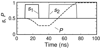
Figure 5: Preparation of entangled Josephson junctions. The solid and dotted lines are $s_{1}(t)$ and $s_{2}(t)$, respectively, and the dashed curve indicates the probability for the system to be found in the state $(|100\rangle-|010\rangle)/\sqrt{2}$.

Acknowledgements. ANC and MRG were supported by the Research Corporation, and MRG was by NSF CAREER Grant No. DMR-0093217.

References

- Makhlin et al. (2001) Y. Makhlin, G. Schön, and A. Shnirman, Rev. Mod. Phys. 73, 357 (2001).
- Yu et al. (2002) Y. Yu, S. Han, X. Chu, S.-I. Chu, and Z. Wang, Science 296, 889 (2002).
- Martinis et al. (2002) J. M. Martinis, S. Nam, J. Aumentado, and C. Urbina, Phys. Rev. Lett. 89, 117901 (2002).
- Berkley et al. (1998) A. J. Berkley, H. Xu, R. C. Ramos, M. A. Gubrud, F. W. Strauch, P. R. Johnson, J. R. Anderson, A. J. Dragt, C. J. Lobb, and F. C. Wellstood, Science 300, 1548 (1998).
- Nakamura et al. (1999) Y. Nakamura, Y. Pashkin, and J. Tsai, Nature 398, 786 (1999).
- Nakamura et al. (2002) Y. Nakamura, Y. Pashkin, and J. Tsai, Phys. Rev. Lett. 88, 047901 (2002).
- Vion et al. (2002) D. Vion, A. Aassime, A. Cottet, P. Joyez, H. Pothier, C. Urbina, D. Esteve, and M. H. Devoret, Science 296, 886 (2002).
- Leggett (2002) A. J. Leggett, Science 296, 861 (2002).
- Shnirman et al. (1997) A. Shnirman, G. Schön, and Z. Hermon, Phys. Rev. Lett. 79, 2371 (1997).
- Makhlin et al. (1999) Y. Makhlin, G. Schön, and A. Shnirman, Nature 398, 305 (1999).
- Mooij et al. (1999) J. E. Mooij, T. P. Orlando, L. S. Levitov, L. Tian, C. H. van der Wal, and S. Lloyd, Science 285, 1036 (1999).
- Makhlin et al. (2000) Y. Makhlin, G. Schön, and A. Shnirman, J. Low. Temp. Phys. 118, 751 (2000).
- You et al. (2002) J. Q. You, J. S. Tsai, and F. Nori, Phys. Rev. Lett. 89, 197902 (2002).
- Plastina and Falci (2003) F. Plastina and G. Falci, Phys. Rev. B 67, 224514 (2003).
- Blais et al. (2003) A. Blais, A. M. van den Brink, and A. M. Zagoskin, Phys. Rev. Lett. 90, 127901 (2003).
- (16) A. Y. Smirnov and A. M. Zagoskin, cond-mat/0207214 (unpublished).
- Buisson and Hekking (2001) O. Buisson and F. W. J. Hekking, in Macroscopic Quantum Coherence and Quantum Computing, edited by D. V. Averin, B. Ruggiero, and P. Silvestrini (Kluwer, New York, 2001), p. 137.
- Marquardt and Bruder (2001) F. Marquardt and C. Bruder, Phys. Rev. B 63, 54514 (2001).
- Armour et al. (2002) A. D. Armour, M. P. Blencowe, and K. Schwab, Phys. Rev. Lett. 88, 148301 (2002).
- Yang et al. (2000) J. Yang, T. Ono, and M. Esashi, Appl. Phys. Lett. 77, 3860 (2000).
- Barone and Paterno (1982) A. Barone and G. Paterno, Physics and Applications of the Josephson Effect (Wiley, New York, 1982).
- Fulton and Dunkleberger (1974) T. A. Fulton and L. N. Dunkleberger, Phys. Rev. B 9, 4760 (1974).
- Ruby and Merchant (1994) R. Ruby and P. Merchant, IEEE Intl. Freq. Control Symposium p. 135 (1994).
- Ruby et al. (2001) R. Ruby, P. Bradley, J. Larson, Y. Oshmyansky, and D. Figueredo, Technical Digest of the 2001 IEEE International Solid-State Circuits Conference pp. 120–121 (2001).
- Cleland et al. (2001) A. N. Cleland, M. Pophristic, and I. Ferguson, Appl. Phys. Lett. 79, 2070 (2001).
- (26) AlN has a density g/cm3, piezoelectric modulus = 1.46 C/m2, and dielectric constant = 10.7 . The resonator has a geometric capacitance fF and a resonance frequency 10 GHz.
- Auld (1990) B. Auld, Acoustic Fields and Waves in Solids (Wiley and Sons, New York, 1990), 2nd ed.
- Scully and Zubairy (1997) M. O. Scully and M. S. Zubairy, Quantum Optics (Cambridge University Press, Cambridge, 1997).
- Maître et al. (1997) X. Maître, E. Hagley, G. Nogues, C. Wunderlich, P. Goy, M. Brune, J. M. Raimond, and S. Haroche, Phys. Rev. Lett. 79, 769 (1997).
- Hagley et al. (1997) E. Hagley, X. Maitre, G. Nogues, C. Wunderlich, M. Brune, J. M. Raimond, and S. Haroche, Phys. Rev. Lett. 79, 1 (1997).