Indirect Exchange Interaction between two Quantum Dots in an Aharonov-Bohm Ring

Abstract

We investigate the Ruderman-Kittel-Kasuya-Yosida (RKKY) interaction between two spins located at two quantum dots embedded in an Aharonov-Bohm (AB) ring. In such a system the RKKY interaction, which oscillates as a function of the distance between two local spins, is affected by the flux. For the case of the ferromagnetic RKKY interaction, we find that the amplitude of AB oscillations is enhanced by the Kondo correlations and an additional maximum appears at half flux, where the interaction is switched off. For the case of the antiferromagnetic RKKY interaction, we find that the phase of AB oscillations is shifted by $\pi$, which is attributed to the formation of a singlet state between two spins for the flux value close to integer value of flux.

I introduction

When two magnetic moments are embedded in a metal, they induce spin polarization in a conduction electron sea and couple each other even they are spatially apart. Such indirect exchange interaction, the Ruderman-Kittel-Kasuya-Yosida (RKKY) interaction, has been known from the 1950s Kittel (1968). The indirect exchange interaction in magnetic nanostructures is one of basic mechanisms for spintronics Maekawa and Shinjo (2002) and it is well understood for ferromagnet and nonmagnetic metal multilayer structures Bruno (1995). However for semiconductor nanostructures, the indirect exchange interaction between local spins formed in two quantum dots has not yet been observed, in spite of the importance as a basic physics and the potential application for semiconductor nanospintronics.

Recent improvement of the fabrication technique for semiconductor nanostructures enables one to make rather complicated structures with possibility of the precise controlling of their parameters. For example, a double quantum dot (QD) system Holleitner et al. (2001) and the composite system of QD and an Aharonov-Bohm (AB) ring have been made Yacoby et al. (1995); Kobayashi et al. (2002). The double-dot system was proposed for a candidate of the “qubit”, because in the Coulomb blockade (CB) regime a dot with odd numbers of electrons, behaves as a local spin and two dot spins can be entangled by introducing the exchange interaction between them Loss and Sukhorukov (2000). Such exchange interaction has been also discussed from the point of view of the competition between the Kondo effect and the antiferromagnetic (AF) interaction Georges and Meir (1999). However the direct exchange interaction was considered rather than the RKKY interaction. Investigations on the AB ring embedded with QD are aimed at understanding the coherent transport through QD Yacoby et al. (1995); König and Gefen (2001, 2002) and the indirect exchange interaction between two local spins has not been addressed.

So it is intriguing to investigate the RKKY interaction between two QDs in CB regime embedded in AB ring. We will show that the RKKY interaction, the sign of which oscillate as a function of the distance (RKKY oscillations), is affected by the flux and it dominates the transport properties. For ferromagnetic (F) coupling between dot spins, the amplitude of AB oscillations is enhanced by Kondo correlations and an additional maximum appears at half flux. For AF coupling case, the phase of AB oscillations is shifted by $\pi$.

II model and calculations

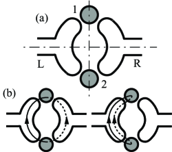
Figure 1: (a) Aharonov-Bohm ring embedded with one QD in each arm. The system has the parity symmetry along the horizontal and vertical axes (dot-dashed lines). (b) The flux dependent (left panel) and independent (right panel) particle-hole excitation. $\Phi$ is the flux penetrating the ring. The directed solid and dashed lines are the particle and hole propagators, respectively.

Figure 1(a) shows the schematic picture of an AB ring embedded with one QD in each arm. QDs denoted with 1 and 2 weakly couple to left and right leads. The effective Hamiltonian is written with two single-channel 1-dimensional (1D) leads Hamiltonian $H_{0}$ and the tunneling Hamiltonian $H_{\rm T}$ as $H=H_{0}+H_{\rm T}$. The lead Hamiltonian is given by $H_{0}=\sum_{k\,r=L,R\,\sigma}\varepsilon_{k}a_{kr\sigma}^{{\dagger}}a_{kr\sigma}$, where $a_{kL(R)\sigma}$ is an annihilation operator of an electron with quantum number $k$ and spin $\sigma$ in the left (right) lead. For simplicity, we adopt the so-called Coqblin-Schrieffer model,

$$H_{\rm T}=\sum_{\stackrel{{\scriptstyle\scriptstyle{r,r^{\prime}=L,R}}}{{n=1,2}}}\sum_{\sigma,\sigma^{\prime}=\uparrow,\downarrow}\frac{J}{2}a_{rn\sigma}^{\dagger}X^{n}_{\sigma^{\prime}\,\sigma}a_{r^{\prime}n\sigma^{\prime}},$$ (1)

for the tunneling Hamiltonian through QDs with odd numbers of electrons in CB regime. The Hubbard operator $X^{n}_{\sigma^{\prime}\,\sigma}=|n,\sigma^{\prime}\rangle\langle n,\sigma|$ describes the spin state of the $n$-th QD and $J>0$ is a coupling constant. The annihilation operator $a_{rn\sigma}$ is written using the projection $\langle n|kr\rangle$ of wave function of an electron in the lead $r$ with quantum number $k$ at the boundary of the $n$-th QD, as $a_{rn\sigma}\!\!=\!\!\sum_{k}\langle n|kr\rangle\,a_{kr\sigma}$ Bruder et al. (1996).

Here we encounter a problem: One needs to know the proper wave function including the information on the coherent propagation of an electron through arms. Usually the scattering theory Gefen et al. (1984) is suitable for treating the electron coherency. However it is complicated to combine this theory with a theory based on the Hamiltonian in the second-quantization representation. In this paper we circumvent this problem. Rather, we utilize an assumption of parity (mirror) symmetry along the horizontal and the vertical axes (dot-dashed lines in Fig. 1(a)). Namely, the total Hamiltonian is invariant under the interchange of indices $L\leftrightarrow R$ or $1\leftrightarrow 2$. Such approximation will make calculations simple and will contain all important physics. Any deviations from such a symmetry will change the result only quantitatively.

For practical calculations, it is convenient to introduce an annihilation operator of even/odd parity states Jayaprakash et al. (1981) $a_{r\pm\sigma}\!=\!(a_{r1\sigma}\!\pm\!a_{r2\sigma})/\sqrt{2}$, ( $a_{r\pm\sigma}\!\!=\!\!\sum_{k}\langle\pm|k\rangle\,a_{kr\sigma}$, where $|\pm\rangle\!=\!(|1\rangle\!\pm\!|2\rangle)/\sqrt{2}$ ; we dropped the index $r$ from $|kr\rangle$ because of the parity symmetry along the vertical axis). Annihilation operators for even and odd parity states are orthogonal,

$$\left\{a_{rp\sigma},a_{r^{\prime}p^{\prime}\sigma^{\prime}}\right\}=\delta_{rr^{\prime}}\delta_{\sigma\sigma^{\prime}}\delta_{pp^{\prime}},$$

because of the parity symmetry along the horizontal axis.

When magnetic field is applied, an AB phase factor ${\rm e}^{i\phi/2}$ (${\rm e}^{-i\phi/2}$) must be counted in Eq. (1), when electron tunnels through a QD in the clockwise(anticlockwise) direction Hackenbroich and Weidenmüller (1996). The AB phase is written with vector potential $\vec{A}$ as,

$$\phi=\frac{2\pi}{\Phi_{0}}\oint\vec{A}\cdot d\vec{l},$$ (2)

where $\Phi_{0}=hc/e$ is the flux quantum and the line integral is performed along the ring in the clockwise direction. An AB flux breaks the time-reversal symmetry and it generates the main difference between features of the orthodox two-impurity Kondo model Beal-Monod (1969); Jayaprakash et al. (1981); Jones and Varma (1987); Jones et al. (1988, 1989) and the AB ring embedded with one QD in each arm. Here, we note that the magnetic field in leads and QDs is not zero for an experiment and it causes Zeeman splitting of electron spins. In the following discussions, we consider an ideal situation where there is no Zeeman splitting and discuss the effect of AB phase on the indirect exchange coupling and transport properties.

The Hamiltonian for the RKKY interaction can be obtained by the second order perturbation theory in terms of $J/\varepsilon_{\rm F}$, where $\varepsilon_{\rm F}$ is the Fermi energy Kittel (1968); Schwabe et al. (1996):

$$H_{\rm RKKY}=\frac{J_{\rm RKKY}(\phi)}{2}\sum_{\sigma\sigma^{\prime}}X^{1}_{\sigma\sigma^{\prime}}X^{2}_{\sigma^{\prime}\sigma}\;.$$ (3)

The coupling constant $J_{\rm RKKY}(\phi)$ can be written as

$$J_{\rm RKKY}(\phi)=\frac{J^{2}}{2}\,\chi\,(2+2\cos\phi),$$ (4)

where a succeptibility function $\chi$ can be found by the perturbation theory based on the Keldysh Green function technique Schwabe et al. (1996). In the equilibrium, it can be written as

$$J^{2}\chi\!\! = \!\!\frac{1}{4}\,{\rm Re}\!\!\int d\varepsilon d\varepsilon^{\prime}\,\frac{\gamma_{p}(\varepsilon)\gamma_{p}(\varepsilon^{\prime})-\gamma_{p}(\varepsilon)\gamma_{\bar{p}}(\varepsilon^{\prime})}{\varepsilon+i\eta-\varepsilon^{\prime}}$$ (5)

$$\times \!\!\!\left\{f^{+}(\varepsilon)-f^{+}(\varepsilon^{\prime})\right\}\;,$$

where $\eta$ is a positive infinitesimal number and $\gamma_{p}(\varepsilon)=J\sum_{k}\langle p|k\rangle\langle k|p\rangle\,\delta(\varepsilon-\varepsilon_{k})$ is a spectral function of parity $p$ “electron propagator”. The subscript $\bar{p}$ represents the opposite parity of $p$, i.e. $\bar{p}=\pm$ for $p=\mp$. Here, $f^{\pm}(\varepsilon)=1/(1+{\rm e}^{\pm\beta\varepsilon})$ is the electron (hole) Fermi distribution function, and $\beta\equiv T^{-1}$(We use the unit $k_{\rm B}\equiv 1$). In Eq. (4), a phase dependent factor $(2+2\cos\phi)$ appears, which value is related to the four configurations of particle-hole excitations - two of which enclose the flux [left panel of Fig. 1(b)] and pick up a phase factor ${\rm e}^{i\phi}$ or ${\rm e}^{-i\phi}$ and give term $2\cos\phi$, and the others (right panel) are independent of the flux - give term $2$. The Eq. (4) is one of the main results of this paper. It shows that by means of external flux $\phi$ one can control the amplitude of the RKKY interaction but it is impossible to change its sign since $(2+2\cos\phi)\geq 0$.

Since we consider 1D leads, we approximate $\gamma_{p}(\varepsilon)$ as for the 1D free electron gas with the linearized dispersion relation Jayaprakash et al. (1981):

$$\gamma_{\pm}(\varepsilon)\simeq\bar{J}\left[1\pm\cos\left\{k_{\rm F}l\left(1+\frac{\varepsilon}{D}\right)\right\}\right],$$ (6)

where $k_{\rm F}$ is the Fermi wave number and $l$ is the length of an electron path between two QDs. The argument of cosine function is the energy dependent “orbital phase” Kubala and König (2003), i.e. the accumulated phase during electron propagation between two QDs. We introduced the cut-off energy $D=\hbar v_{\rm F}k_{\rm F}$, where $v_{\rm F}$ is the Fermi velocity. Here, $\bar{J}$ is written with the density of the states $\rho$ as $\bar{J}\equiv J\rho$. Substituting Eq. (6) into Eqs. (4) and (5), we obtain for short distance between two QDs ($k_{\rm F}l\ll 2\pi$) the ferromagnetic coupling as $J_{\rm RKKY}(\phi)\simeq-2\ln 2\,\bar{J}^{2}D\,(2+2\cos\phi)$ and more relevant - the RKKY oscillations of 1D free electron gas Kittel (1968); Yafet (1987) as a function of $l$ for long distance between dots ($k_{\rm F}l\gg 2\pi$)

$$J_{\rm RKKY}(\phi)\simeq-\frac{\pi\bar{J}^{2}D\cos(2k_{\rm F}l)}{4\,k_{\rm F}l}\,(2+2\cos\phi).$$ (7)

Above expressions are obtained by replacing the Fermi functions in Eq. (5) with those at $T\!=\!0$, what is valid below the characteristic temperature $T^{*}$ defined by,

$$T^{*}\equiv\frac{\hbar}{\tau},\;\;\tau\equiv\frac{\hbar k_{\rm F}l}{D}=\frac{l}{v_{\rm F}}.$$ (8)

Here, $\tau$ is the characteristic time scale for an electron travels between two QDs. It can be understood from the following argument: Electrons deep inside the Fermi sea are responsible for the RKKY oscillations. On the other hand, electrons with energy $\varepsilon$ ($|\varepsilon|\ll T^{*}$), i.e. electrons around the Fermi level, are unimportant, because such electrons contribute only oscillations whose characteristic wave length $hv_{\rm F}/T^{*}$ is much longer than $l$. Thus the RKKY oscillations are insensitive to the temperature in the regime $T\ll T^{*}$. However, when the temperate reaches $T^{*}$, the RKKY oscillations are affected by the thermal excitations of lead electrons and will be smeared out.

Due to the RKKY interaction, depending on the sign of the coupling $J_{\rm RKKY}(\phi)$ [Eq. (7)], the two dot spins are entangled and form a singlet state $|0,0\rangle$ for AF coupling ($J_{\rm RKKY}(\phi)>0$) or a triplet state $|1,m\rangle$ ($m=0,\pm 1$) for F coupling ($J_{\rm RKKY}(\phi)<0$).

In the following, we will discuss how the flux dependent RKKY interaction modifies transport properties of the ring. To calculate the conductance, we adopt the third order perturbation theory in terms of $\bar{J}$, in order to take into account the Kondo correlations: They are pronounced when the temperature decreases and approaches the order of the Kondo temperature $T_{\rm K}\!\sim\!D\exp(-1/(2\bar{J}))$. In our case, the RKKY interaction becomes important at the temperature, where the Kondo correlations are also unignorable. First we rewrite the tunnel Hamiltonian, Eq. (1), using the vector operator of the $n$-th local spin $\vec{S}^{n}$, whose components are defined as $S^{n}_{+/-}=X^{n}_{\uparrow\downarrow/\downarrow\uparrow}$ and $S^{n}_{z}=(X^{n}_{\uparrow\uparrow}-X^{n}_{\downarrow\downarrow})/2$. Further we introduce operators $\vec{S}^{\pm}=\vec{S}^{1}\pm\vec{S}^{2}$, which satisfy the following commutation relations:

$$[S^{p}_{i},S^{p}_{j}]=i\epsilon_{ijk}S^{+}_{k},\;\;[S^{p}_{i},S^{\bar{p}}_{j}]=i\epsilon_{ijk}S^{-}_{k},$$ (9)

where $\epsilon_{ijk}$ is the Levi-Chivita antisymmetric tensor. The operator $\vec{S}^{+}$ does not change the total spin-quantum number, while $\vec{S}^{-}$ is the operator of the singlet-triplet transition. By using above operators, we obtain the symmetrized form of $H_{\rm T}$ Beal-Monod (1969); Matho and Beal-Monod (1972); Jayaprakash et al. (1981) taking into account the AB phase as

$$H_{\rm T}\!\! = \!\!\frac{J}{4}\!\!\!\sum_{\stackrel{{\scriptstyle\scriptstyle{p=\pm}}}{{\sigma,\sigma^{\prime}=\uparrow,\downarrow}}}\left\{\sum_{r}\left(\vec{\sigma}_{rr}^{p}\!\!\cdot\vec{S}^{p}+v\,a_{rp\sigma^{\prime}}^{\dagger}\delta_{\sigma^{\prime}\sigma}a_{rp\sigma}\right)\right.$$

$$+ \!\!\!\cos\frac{\phi}{2}\left(\vec{\sigma}_{RL}^{p}\!\!\cdot\vec{S}^{p}+v\,a_{Rp\sigma^{\prime}}^{\dagger}\delta_{\sigma^{\prime}\sigma}a_{Lp\sigma}\right)\!\!+\!{\rm H.c.}$$

$$+ \!\!\!\left.i\sin\frac{\phi}{2}\left(\vec{\sigma}_{RL}^{\bar{p}}\!\!\cdot\vec{S}^{p}+v\,a_{R\bar{p}\sigma^{\prime}}^{\dagger}\delta_{\sigma^{\prime}\sigma}a_{Lp\sigma}\right)\!\!+\!{\rm H.c.}\right\}.$$

Here, $\vec{\sigma}^{+(-)}_{r^{\prime}r}=\sum_{\sigma\sigma^{\prime}p}a_{r^{\prime}p\sigma^{\prime}}^{\dagger}\vec{\sigma}_{\sigma^{\prime}\sigma}a_{rp(\bar{p})\sigma}$ denotes effective conducting electron spin and is defined with the vector Pauli matrix $\vec{\sigma}$. Terms proportional to $v$ represent potential scattering process and for our case, $v=1$. The first line represents the reflection process and shows that the change of parity and the singlet-triplet transition occur simultaneously. The second and the third lines describe transmission processes. The third line describes the singlet-triplet transition without changing the parity, that is not invariant under the interchange of indices, $L\leftrightarrow R$ or $1\leftrightarrow 2$, (i.e. the replacement of $a_{{\rm r}\pm\sigma}$ with $\pm a_{{\rm r}\pm\sigma}$). Here it does not mean that the parity symmetry is broken: the space inversion transformation changes $\phi\rightarrow-\phi$, because it also reverses the direction of the line integral in Eq. (2).

In order to calculate the linear conductance, we adopt the diagrammatic technique for the density matrix in the real-time domain Schoeller and Schön (1994); König et al. (1996). With the help of the commutation relations, Eq. (9), the perturbative calculation is performed rather systematically (Appendix. A). The “partial self-energy” which represents the transition rate for an electron from the left lead to the right lead accompanied by the triplet-triplet transition $\Sigma^{LR}_{11}$ or preserving a singlet state $\Sigma^{LR}_{00}$ or accompanied by the singlet-triplet transition $\Sigma^{LR}_{j\bar{j}}$ ($j=0,1$) is obtained as follows:

$$\Sigma^{LR}_{11} \simeq \frac{3\pi i}{2}\,\int d\varepsilon\sum_{p=\pm}\left[\gamma^{+}_{pL}(\varepsilon)\,\gamma^{-}_{pR}(\varepsilon)\,{\rm Re}\left\{1+\frac{v^{2}}{2}+\sigma_{1\,p}(\varepsilon)+\sum_{j=0,1}\frac{\sigma_{1\,\bar{p}}(\varepsilon-\Delta_{j\bar{j}})}{2}\right\}\cos^{2}\frac{\phi}{2}\right.$$

$$+ \left.\gamma^{+}_{pL}(\varepsilon)\,\gamma^{-}_{\bar{p}R}(\varepsilon)\,{\rm Re}\left\{1+\frac{v^{2}}{2}+\sigma_{0\,p}(\varepsilon)+\sum_{j=0,1}\frac{\sigma_{0\,\bar{p}}(\varepsilon-\Delta_{j\bar{j}})}{2}\right\}\sin^{2}\frac{\phi}{2}\right],$$

(11)

$$\Sigma^{LR}_{00} \simeq \frac{\pi i}{4}\,\int d\varepsilon\sum_{p=\pm}v^{2}\biggl{\{}\gamma^{+}_{pL}(\varepsilon)\,\gamma^{-}_{pR}(\varepsilon)\,\cos^{2}\frac{\phi}{2}+\gamma^{+}_{pL}(\varepsilon)\,\gamma^{-}_{\bar{p}R}(\varepsilon)\,\sin^{2}\frac{\phi}{2}\biggl{\}},$$ (12)

$$\Sigma^{LR}_{j\bar{j}} \simeq \frac{3\pi i}{4}\int d\varepsilon\sum_{p=\pm}\left[\gamma^{+}_{pL}(\varepsilon)\,\gamma^{-}_{\bar{p}R}(\varepsilon-\Delta_{\bar{j}j})\,{\rm Re}\left\{1+\sigma_{1\,p}(\varepsilon)+\sigma_{1\,\bar{p}}(\varepsilon-\Delta_{\bar{j}j})\right\}\cos^{2}\frac{\phi}{2}\right.$$ (13)

$$+ \left.\gamma^{+}_{pL}(\varepsilon)\,\gamma^{-}_{pR}(\varepsilon-\Delta_{\bar{j}j})\,{\rm Re}\left\{1+\sigma_{0\,p}(\varepsilon)+\sigma_{0\,\bar{p}}(\varepsilon-\Delta_{\bar{j}j})\right\}\sin^{2}\frac{\phi}{2}\right],$$

where we neglected the integral ${\rm Re}\int d\varepsilon^{\prime}\gamma_{p}(\varepsilon^{\prime})/(\varepsilon+i\eta-\varepsilon^{\prime})$. The subscript $j=1(0)$ denotes the total-spin quantum number and $\bar{j}=0(1)$. Here $\Delta_{10}=-\Delta_{01}=J_{\rm RKKY}(\phi)$ and $\gamma_{pr}^{\pm}(\varepsilon)=\gamma_{p}(\varepsilon)f^{\pm}(\varepsilon-\mu_{r})$ denotes the “lesser” or “greater” Green function where $\mu_{L}=-\mu_{R}=eV/2$. The function $\sigma_{0(1)p}$ defined by

$$\sigma_{0(1)p}(\varepsilon)=\int d\varepsilon^{\prime}\frac{\gamma^{+}_{Lp}(\varepsilon^{\prime})+\gamma^{+}_{R\bar{p}(p)}(\varepsilon^{\prime})}{\varepsilon+i\eta-\varepsilon^{\prime}},$$ (14)

gives the logarithmic divergence related with Kondo correlations. By substituting Eq. (6) to Eq. (14), we obtain

$$\sigma_{0\pm}(\varepsilon)\!\! \simeq \!\!2\bar{J}\ln\frac{2{\rm e}^{\gamma}D}{\pi T},$$

$$\sigma_{1\pm}(\varepsilon)\!\! \simeq \!\!\sigma_{0\pm}(\varepsilon)\pm 2\bar{J}\,{\rm Re}\biggl{[}{\rm e}^{ik_{\rm F}l}\biggl{\{}\ln\frac{2T^{*}}{\pi T}$$

$$+ {\rm Ei}\left(-ik_{\rm F}l\right)\biggl{\}}\biggl{]},$$

for $V=0$ and $\varepsilon\ll T,T^{*}$. Here ${{\rm Ei}(x)}$ denotes the exponential integral function and $\gamma\approx 0.577$ is the Euler constant. Equation (4) supplemented with Eq. (5) and Eqs. (11), (12) and (13) are main results of this paper.

Using the partial self-energy, Eqs. (11), (12) and (13), the current can be expressed as

$$I=-\frac{ie}{\hbar}\sum_{j,j^{\prime}=0,1}P_{j}\,\left\{\Sigma^{LR}_{j\,j^{\prime}}-(L\leftrightarrow R)\right\},$$ (15)

where probabilities $P_{0}$ for a singlet state and $P_{1}$ for each of particular triplet states (we consider no Zeeman splitting), can be obtained for the linear response from the Boltzmann distribution as

$$P_{0}=\frac{1}{1+3\,\exp(-\beta J_{\rm RKKY}(\phi))},\;\;P_{1}=\frac{1-P_{0}}{3}\;.$$ (16)

The linear conductance is defined as $G=\lim_{V\rightarrow 0}\partial I/\partial V$.

III results and discussion

For the AB ring geometry without quantum dots in arm, the conductance oscillates as a function of the flux $\phi$ Gefen et al. (1984). Furthermore, because of the orbital phase, the conductance also oscillates as a function of the length of the arm $l$ for enough low temperatures: As the thermal excitation of lead electrons scrambles various orbital phases, the oscillatory component would be reduced for temperatures above the characteristic temperature $T^{*}$, where characteristic length $hv_{\rm F}/T$ reaches $l$. When one local spin, i.e. QD, is embedded in each arm of the AB ring, in addition to the oscillatory component, the non-oscillatory background of oscillations related to spin-flip processes will appear: Spin-flip processes do not contribute to the interference effect Akera (1993) because if a local spin is flipped, we can determine the path which an electron propagated. Such non-oscillatory background reduces the portion of oscillatory component. However, if we take account of the RKKY interaction, the oscillatory component can be enhanced from the following mechanism: First, according to Eq. (16), the probabilities for singlet $P_{0}$ and triplet $P_{1}$ states will be affected by the RKKY coupling constant $J_{\rm RKKY}(\phi)$, which is a oscillatory function in terms of $\phi$ and $l$. Second, as the conductance would be sensitive to a state of local spins, it would show also the oscillatory behavior related to the oscillations of $J_{\rm RKKY}(\phi)$. Such RKKY dominant oscillations one could expect for the enough low temperature $T\!\ll\!|J_{\rm RKKY}(0)|\!\ll\!T^{*}$.

In the following, we will discuss the properties of our system for temperatures where the thermal scrambling of orbital phases is unimportant $T\!\ll\!T^{*}$ and above the Kondo temperature $T\!\gg\!T_{\rm K}$. We note that as $|J_{\rm RKKY}(\phi)|\!\ll\!T^{*}$, the modification of orbital phases by inelastic spin-flip scattering events is also unimportant.

III.1 $l$ - dependence

First we will discuss the RKKY oscillations without magnetic flux $\phi=0$ as a function of the distance $l$ between two QDs. Figure 2(a) shows the RKKY oscillations of the coupling constant $J_{\rm RKKY}(0)$ as a function of the length of an electron path $l$. It oscillates with the period of $k_{F}l/\pi=1$, and shows local minima at integer values of $k_{\rm F}l/\pi$ corresponding to ferromagnetic (F) coupling and local maxima at half-integer values of $k_{\rm F}l/\pi$ corresponding to the antiferromagnetic (AF) coupling between the spins. The amplitude of the oscillations decay with $~{}1/k_{\rm F}l$ as predicted for RKKY interaction in quasi 1D geometry Yafet (1987). In Figure 2(b), there is a plot of the probability $P_{0}$ of the singlet state. At low temperature $T\lesssim|J_{\rm RKKY}(0)|$ (the solid line), a singlet state (triplet state) is formed when value of $k_{\rm F}l/\pi$ is close to half-integer (integer). As the temperature increases (the dashed line for $T\sim|J_{\rm RKKY}(0)|$ and the dotted line for $T\gg|J_{\rm RKKY}(0)|$) the amplitude of oscillations is suppressed and system approaches uniform distribution between the singlet and triplet states - $P_{0}=P_{0}=1/4$. There are also the oscillations of the conductance [Fig. 2(c)] with the period of $k_{\rm F}l/\pi=1$. In the same way as in Fig. 2(b), the amplitude of oscillations is suppressed for $T\gg|J_{\rm RKKY}(0)|$, what indicates that in regime $T<|J_{\rm RKKY}(0)|$ the conductance oscillations are mainly determined by the RKKY interaction. Experimentally, it can be difficult to control the length of arms keeping other parameters fixed. However, the conductance oscillations would be possible to observe by changing the Fermi wave number $k_{\rm F}$, by controlling the carrier density of 2D electron gas (2DEG) with an additional gate.

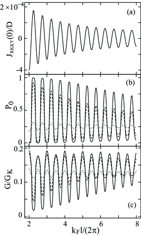
Figure 2: Length dependent (a) RKKY coupling constant, (b) probability for singlet state and (c) conductance for $T/D=5\times 10^{-5}$ (solid line), $10^{-4}$ (dashed line) and $10^{-3}$ (dotted line). Parameters are taken as $\phi=0$ and $\bar{J}=0.04$.

III.2 $\phi$ - dependence

Though above discussions suggest that the RKKY interaction dominates the length dependent conductance, it would be more convenient experimentally to measure the flux dependence. In the following we will discuss the modification of AB conductance oscillations by the presence of RKKY interaction.

As we mentioned before by means of external flux $\phi$ one can change the amplitude of the RKKY interaction but not its sign since $(2+2\cos\phi)\geq 0$. In the particular experimental situation depending on the length $l$ of the arm and Fermi wave vector $k_{\rm F}$ the spins can be coupled ferromagnetically or antiferromagnetically. By means of flux $\phi$ one can control the strength of the interaction but does not switch between them. For this reason it is generic to discuss three typical situations, for which we are able to get analytic results. These three cases are classified by the value of the RKKY coupling constant: (i) the uncorrelated local spins case ($\left|J_{\rm RKKY}(\phi)\right|\!\ll\!T$), (ii) the ferromagnetic coupling case ($-J_{\rm RKKY}(\phi)\!\gg\!T$) and (iii) the antiferromagnetic coupling ($J_{\rm RKKY}(\phi)\!\gg\!T$).

(i) Uncorrelated local spins limit is realize for high temperature $\left|J_{\rm RKKY}(\phi)\right|\ll T$ or for the flux $\phi\approx\pi+2\pi n$ since then, according to Eq. (4), the RKKY interaction is weak, $J_{\rm RKKY}(\phi)\rightarrow 0$. In this case (i), the local-spin state is distributed with equal probability among a singlet state and a triplet state $P_{1}\approx P_{0}\approx 1/4$ [see Eq. (16)]. The conductance is expressed as

$$\frac{G}{G_{\rm K}} \simeq (\pi\bar{J})^{2}\biggl{\{}v^{2}\left(1+\cos\phi\,\cos^{2}k_{\rm F}l\right)$$ (17)

$$+ 3\left(1+4\bar{J}\ln\frac{2{\rm e}^{\gamma}D}{\pi T}\right)\biggl{\}},$$

where $G_{\rm K}=e^{2}/h$ is the quantum conductance. The first term, which is proportional to $v^{2}$ and thus independent of spin-flip processes, is attributed to the phase coherent component of the cotunneling process. It shows the ordinary AB oscillations. The second term in Eq. (17), which is related to spin-flip processes (does not depend on $\phi$), form the background of AB oscillations. We can see that with decreasing of temperature the Kondo correlations enhance the background: The second term can be interpreted as the parallel conductance through two independent spin-1/2 local moments whose conductance is enhanced by Kondo correlations not . In the third order contribution in $\bar{J}$ in Eq. (17), there is no interference related to the orbital phase $k_{\rm F}l$, which was pointed out by Beal-Monod Beal-Monod (1969). We explicitly showed by Eq. (17) that there is also no interference related to the AB phase in the third order contribution.

(ii) The ferromagnetic coupling for $-J_{\rm RKKY}(\phi)\gg T$ : In this case, two local spins form a triplet state $P_{1}\approx 1/3$ and $P_{0}\approx 0$ [see Eq. (16)]. Thus, the conductance is that of $S=1$ Kondo model plus the potential scattering. For the case of long distance between QDs ($k_{\rm F}l\gg 1$),

$$\frac{G}{G_{\rm K}} \simeq 2(\pi\bar{J})^{2}\left[4\bar{J}\cos^{2}k_{\rm F}l\,\cos^{2}\frac{\phi}{2}\,\ln\frac{2T^{*}}{\pi T}\right.$$

$$+ \left.\left(1+\frac{v^{2}}{2}+2\bar{J}\ln\frac{2{\rm e}^{\gamma}D}{\pi T}\right)\left(1+\cos\phi\,\cos^{2}k_{\rm F}l\right)\right].$$

For the opposite case, $k_{\rm F}l\ll 1$, we obtain the same equation as Eq. (LABEL:eqn:approx2) with replacing $T^{*}$ in the logarithm by ${\rm e}^{-\gamma}D$. The striking feature is that as opposed to the case (i), the Kondo correlations enhance the oscillatory component as it is shown in the second term of Eq. (LABEL:eqn:approx2). Loosely speaking, two spins are no longer independent phase-breaking scatterers because they “observe” each other and the Kondo correlations enhances the AF coupling of each QD spin to the conducting electrons spins. The first term of Eq. (LABEL:eqn:approx2) shows the logarithmic divergence, whose the cutoff energy is equal to the characteristic temperature of the orbital phase coherence $T^{*}$. This term appears because the spin-1 moment stretches over $l$. Using Eq. (LABEL:eqn:approx2), we can relate the F coupling of spins by RKKY interaction [Fig. 2(a)] with the maximum in the conductance [Fig. 2(c)] around integer values of $k_{\rm F}l/\pi$.

(iii) The antiferromagnetic coupling, $J_{\rm RKKY}(\phi)\!\gg\!T$: In this case two local moments form a singlet state $P_{1}\!\approx\!0$ and $P_{0}\!\approx\!1$ [see Eq. (16)]. As the singlet state is decoupled form lead electrons, i.e. electrons flowing through QDs cannot excite local spins to a triplet state, so only the potential scattering process contributes to the conductance:

$$G/G_{\rm K}\simeq(\pi\bar{J})^{2}\,v^{2}(1+\cos\phi\,\cos^{2}k_{\rm F}l).$$ (19)

Because we consider the Coulomb blockade regime, the cotunneling current is very small. It is the reason why the conductance is suppressed around each half integer value of $k_{\rm F}l/\pi$ [Fig. 2(c)], where the RKKY coupling is antiferromagnetic [Fig. 2(a)]. Here we note that situation (ii) and (iii) are not realized for the flux $\phi\approx\pi+2\pi n$ since $J_{\rm RKKY}(\phi)$ is small there and the limit (i) is approached. For $|J_{\rm RKKY}(0)|>T$ by means of the flux $\phi$ we can tune between (ii) and (i), or (iii) and (i) but not between (ii) and (iii) situations.

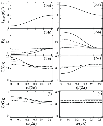
Figure 3: Flux dependent RKKY coupling constant ((1-a) and (2-a)), probability for singlet state((1-b) and (2-b)) and conductance ((1-c) and (2-c)) for $\bar{J}=0.04$. Panels (1-a), (1-b) and (1-c) correspond to the F coupling case ($k_{\rm F}l/(2\pi)=5$) and panels (2-a), (2-b) and (2-c) correspond to AF coupling case ($k_{\rm F}l/(2\pi)=5.25$). Flux dependent conductance for (3) $k_{\rm F}l/(2\pi)=50$ and (4) $50.25$. The solid, dashed, dotted, and dot-dashed lines show the results for $T/D=5\times 10^{-5},10^{-4},2\times 10^{-4}$, and $10^{-3}$, respectively.

For above three cases, we obtained simple analytic results and clarify that the local-spin state due to RKKY interaction causes the pronounced effect on the conductance. Next, we will analyze the conductance of the system for the full range of the flux $\phi$ and discuss the additional structures caused by the flux dependent RKKY interaction, which can be an evidence of the RKKY interaction in our system. Figures 3(1-a) and (2-a) show the RKKY coupling constant $J_{\rm RKKY}(\phi)$ as a function of the flux $\phi/(2\pi)$. The former shows plot for F coupling case ($k_{\rm F}l/\pi$ is an integer) and the latter show the plot for AF coupling case ($k_{\rm F}l/\pi$ is a half-integer). The panels (1-b) and (2-b) are the corresponding plots of the probability for the singlet state for various temperatures and the panels (1-c) and (2-c) are plots of the conductance. In the vicinity of zero flux $\pi=0$, electron wave functions constructively interfere and thus the maximum RKKY interaction is induced [panels (1-a) and (2-a)]. For F coupling case, a triplet state is formed, i.e. $P_{0}\sim 0$, at low temperature [panel (1-b)] and thus the conductance is enhanced [panel (1-c)] as discussed in (ii). For AF coupling case at low temperature, a singlet is formed [panel (2-b)] and the conductance is suppressed [panel (2-c)] as it was discussed in (iii). At half flux, electron wave functions destructively interfere and the RKKY interaction is switched off [panels (1-a) and (2-a)]. Surprisingly at half flux we can observed the maximum in the conductance for both situations F and AF. According to discussion in (i), this maximum is caused by the term in Eq. (17), which does not depend on the flux, and which corresponds to incoherent transport thought the two independent spin-1/2 local moments related to Kondo correlations. Especially for AF coupling case, it leads to the effective phase shift of AB conductance oscillations by $\pi$ [panels (2-c)].

In order to compare our results with the limit, where the RKKY interaction is negligible, we show curves of AB oscillations for $|J_{\rm RKKY}(\phi)|\ll T$ in panels (3) and (4). As discussed in (i), the component of the ordinary AB oscillations is very small. The Kondo correlations only enhance the background and they do not promote characteristic structures as the case of the AF or F coupling.

Here we note some features to distinguish experimentally the RKKY dominant oscillations from the ordinary AB oscillations. The first feature is the characteristic temperature below which the oscillations can be observed: The characteristic temperature of the ordinary AB oscillations $T^{*}$ is higher than that of RKKY dominant oscillations $|J_{\rm RKKY}(0)|$ by the factor $\sim\!\bar{J}^{-2}$. One can point out that the RKKY dominant oscillations is sensitive to the temperature. The second feature is the temperature dependence of the amplitude of oscillations: Suppose we decrease the temperature from enough high temperature $T\gg|J_{\rm RKKY}(0)|$, where singlet and triplet probabilities are $P_{1}\!\approx P_{1}\!\approx 1/4$ and the conductance is expressed by Eq. (17). As temperature is lowered, singlet and triplet probabilities are modified as $P_{0}\approx 1/4\,(1-3J_{\rm RKKY}(\phi)/(4T))$ and $P_{1}\approx 1/4\,(1+J_{\rm RKKY}(\phi)/(4T))$. Therefore, the correction depending on both the orbital phase and the AB phase

$$\delta G\! \simeq \!\!-(\pi\bar{J})^{2}\biggl{\{}3\!\left(1+4\bar{J}\ln\frac{2{\rm e}^{\gamma}D}{\pi T}\right)(2+\cos^{2}k_{\rm F}l\cos\phi)$$

$$+ 2v^{2}(1+\cos^{2}k_{\rm F}l\cos\phi)\biggl{\}}\frac{J_{\rm RKKY}(\phi)}{4T},$$

emerges. It grows as $\propto(\ln T)/T$; the logarithmic correction is related to the Kondo correlations. We expect that with the help of the Kondo correlations one can distinguish the RKKY dominant AB conductance oscillations from the ordinary AB oscillations.

Here we will note on the Onsager symmetry. For the two-terminal geometry, it means that the conductance is an even function of the flux. We can see that the RKKY coupling constant $J_{\rm RKKY}(\phi)$ is an even function of the flux (Eq. (4)). This property depends only on the symmetry of the Hamiltonian under the inversion of time and magnetic field Kubo et al. (1985) and does not depends on the assumption of the mirror symmetry.

Finally we discuss on the range of parameters. For a 2 DEG system at an AlAs/GaAs heterostructure, the carrier density of which is typically $\approx 3.8\times 10^{15}{\rm m}^{-2}$Kobayashi et al. (2002), the Fermi energy and the Fermi wave length are $\varepsilon_{\rm F}\!\approx\!D\!\approx\!14\,{\rm meV}$ and $2\pi/k_{\rm F}\!\approx\!40\,{\rm nm}$, respectively. The RKKY coupling constant $J_{\rm RKKY}(0)\!\!\sim\!\!\bar{J}^{2}D/(k_{\rm F}l)$ should be larger than the Kondo temperature $T_{\rm K}\!\sim\!D\exp(-1/(2\bar{J}))$, $|J_{\rm RKKY}(0)|\!\gg\!T_{\rm K}$, otherwise, each spin-1/2 local moment forms Kondo singlet and are screened out and thus the RKKY interaction is unimportant. In our calculations, we put $\bar{J}=0.04$ which gives the small Kondo temperature, $T_{\rm K}\sim 3.7\times 10^{-6}D\ll|J_{\rm RKKY}(0)|$. Because we adopted the perturbation theory, the temperature should be above the Kondo temperature, $T\gg T_{\rm K}$. In order to obtain the large RKKY interaction $J_{\rm RKKY}(0)\gtrsim T$ we put the size of the ring as $k_{\rm F}l\approx 5\times 2\pi$ (about 200 nm).

For the case of a small AB ring, the Zeeman splitting could become important. In order to reduce the Zeeman splitting $E_{Z}$ keeping the number of fluxes constant, one could increase the size of the AB ring because $J_{\rm RKKY}(0)/E_{\rm Z}\sim l$. In such a case, the consideration of the Kondo regime $T\lesssim T_{\rm K}$, could be needed because RKKY interaction was also reduced so the limit $T_{K}\gtrsim|J_{\rm RKKY}(0)|$ was approached.

IV summary

In conclusion, we have theoretically investigated the RKKY interaction acting between local spins, i.e. two QDs with odd numbers of electrons in CB regime, embedded in the AB ring. We assumed the parity symmetry of the system and such an assumption does not change the result qualitatively. We calculated the RKKY coupling constant and the conductance above the Kondo temperature, $T\gg T_{\rm K}$. The RKKY coupling constant, the sign of which oscillates as a function of the distance, also depends on the flux and the distance between two QDs. When the RKKY interaction is ferromagnetic, two local spins form a triplet state around zero flux, where the electron wave constructively interfere, and thus the maximum RKKY interaction is induced. As the temperature decreases, the amplitude of AB oscillations is enhanced by Kondo correlations, which is the distinctive difference between the ordinary AB oscillations and those of the ferromagnetically coupled two local spins. The maximum was found at half flux where the RKKY interaction is switched off and the conductance is described by the parallel conductance of two independent spin-1/2 local moments whose conductance is enhanced by Kondo correlations. When the RKKY interaction is AF, the phase of AB oscillations is shifted by $\pi$. It is because around zero flux, where we obtain the maximum AF interaction, two local spins form a singlet state, which is decoupled from the lead electrons.

Appendix A third order perturbation theory

In this Appendix, we present detailed calculations of the third-order partial self-energy in terms of $\bar{J}$ on the basis of the diagrammatic technique in the real-time domain Schoeller and Schön (1994); König et al. (1996). Figure 4 shows the second order diagrams for the partial self-energy representing the transition preserving the total-spin quantum number $j$, $\Sigma^{LR}_{jj}$ ((a-1), (a-2) and (a-3)) and the singlet-triplet transition, $\Sigma^{LR}_{j\bar{j}}$ ($j=0,1$) ((b-1) and (b-2)). Green functions of lead electrons are represented by directed solid lines, which are also called “reservoir lines”, and solid lines on the Keldysh contour (two horizontal lines) represents propagators of local spins. Here diagrams (a-1) and (a-3) represent different processes. For the former case, we must count factor $-1$ for the vertex denoted with $S^{+}_{z}$ when $\sigma=\downarrow$. We omitted diagrams which could be obtained by applying the mirror rule König (unpublished).

Following the rules in Ref. Schoeller and Schön (1994), the diagram (a-1) plus its mirror diagram can be calculated as

$${\Sigma^{LR}_{jj}}^{\text{(a-1)}}\!\!\! = \!\!\!\sum_{\stackrel{{\scriptstyle\scriptstyle{p=\pm}}}{{-j\leq m\leq j}}}\!\!\!\!\frac{i\pi}{8}\int d\varepsilon\gamma^{+}_{pL}(\varepsilon)\gamma^{-}_{pR}(\varepsilon)\cos^{2}\!\frac{\phi}{2}$$ (20)

$$\times {\rm Re}\,\langle j,m|2{S^{+}_{z}}^{2}|j,m\rangle.$$

The results for the diagrams (a-2) and (a-3), which we term ${\Sigma^{LR}_{jj}}^{\text{(a-2)}}$ and ${\Sigma^{LR}_{jj}}^{\text{(a-3)}}$, can be obtained from Eq. (20) by changing $2{S^{+}_{z}}^{2}$ to $S^{+}_{\pm}S^{+}_{\mp}$ and to $2v^{2}$, respectively. In the same way, the diagram (b-1) plus its mirror diagram is calculated as

$${\Sigma^{LR}_{j\bar{j}}}^{\text{(b-1)}}\!\!\! = \!\!\!\sum_{\stackrel{{\scriptstyle\scriptstyle{p=\pm}}}{{-j\leq m\leq j}}}\!\!\!\frac{i\pi}{8}\int d\varepsilon\gamma^{+}_{pL}(\varepsilon)\gamma^{-}_{\bar{p}R}(\varepsilon-\Delta_{j\bar{j}})\cos^{2}\!\!\frac{\phi}{2}$$ (21)

$$\times {\rm Re}\,\langle j,m|2{S^{-}_{z}}^{2}|j,m\rangle,$$

where $\Delta_{j\bar{j}}$ is the energy difference between the total-spin quantum number $j$ state and $\bar{j}$ state. The result for the diagram (b-2), which we denote by ${\Sigma^{LR}_{j\bar{j}}}^{\text{(b-2)}}$, is obtained from Eq. (21) by replacing of $2{S^{-}_{z}}^{2}$ by $S^{+}_{\pm}S^{+}_{\mp}$.

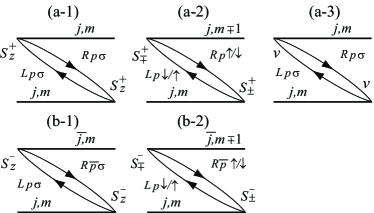
Figure 4: The diagrams for the second order partial self-energy representing the transition preserving total-spin quantum number $j$, [(a-1), (a-2) and (a-3)] and the singlet-triplet transition [(b-1) and (b-2)]. Directed lines represent propagators for lead electrons. Thick solid lines on the Keldysh contour (two horizontal lines) represent propagators for the local spins.

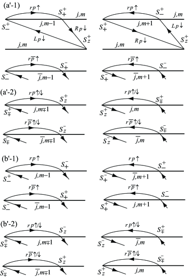
Figure 5: The third order diagrams: Each four diagrams of (a’-1), (a’-2), (b’-1) and (b’-2) show corrections for the vertex on the upper branch of the diagram (a-1), (a-2), (b-1) and (b-2) in Fig. 4, respectively.

The third order diagrams give the vertex correction to the second order diagrams. Figures 5(a’-1), (a’-2), (b’-1) and (b’-2) show the correction for the vertex on the upper branch of diagrams (a-1), (a-2), (b-1) and (b-2) in Fig. 4, respectively. Except for the topmost two diagrams, we omitted the lower branch of each diagram, which is exactly the same as for the corresponding diagram in Fig. 4. The left diagrams and the right diagrams show direct tunneling processes and exchange processes, respectively. We did not show the correction for the diagram (a-3) because it is proportional to $\sum_{-j\leq m\leq j}\langle j,m|S^{+}_{z}|j,m\rangle$ and thus vanishes. For example, the topmost two diagrams in Fig. 5 plus their mirror diagrams are calculated by utilizing the commutation relations Eq. (9) as

$$\!\!\!{\Sigma^{LR}_{jj}}^{\text{(a-1) correction}}=$$ (22)

$$\frac{2i}{4^{3}}\,{\rm Im}\sum_{r\,p}\int d\varepsilon_{1}d\varepsilon_{2}d\varepsilon_{3}\frac{\gamma^{+}_{Lp}(\varepsilon_{1})\gamma^{-}_{Rp}(\varepsilon_{3})}{\varepsilon_{1}-\varepsilon_{3}+i\eta}\cos^{2}\frac{\phi}{2}$$

$$\times \!\!\!\langle j,m|\,S^{+}_{z}\left\{\frac{\gamma^{-}_{rp}(\varepsilon_{2})\,S_{+}^{+}S_{-}^{+}}{\varepsilon_{1}-\varepsilon_{2}+i\eta}-\frac{\gamma^{+}_{rp}(\varepsilon_{2})\,S_{-}^{+}S_{+}^{+}}{\varepsilon_{2}-\varepsilon_{3}+i\eta}\right\}|j,m\rangle$$

$$\simeq \frac{i\pi}{8}\sum_{p}\int d\varepsilon\gamma^{+}_{Lp}(\varepsilon)\gamma^{-}_{Rp}(\varepsilon)\cos^{2}\frac{\phi}{2}$$

$$\times \!\!\!{\rm Re}\left\{\frac{\sigma_{1p}(\varepsilon)}{4}\langle j,m|2{S^{+}_{z}}^{2}|j,m\rangle\right\},$$

where $\sigma_{1p}$ is defined in Eq. (14). Here we counted the minus sign for a loop with three vertices in the anticlockwise direction and we dropped terms except for the renormalization of the transmission probability. We checked that terms which we dropped are canceled out by the other diagrams than those depicted in Fig. 5, i.e. diagrams in which the position of a lower vertex is inbetween upper two vertices. Further we neglected the integral ${\rm Re}\int d\varepsilon^{\prime}\gamma_{p}(\varepsilon^{\prime})/(\varepsilon+i\eta-\varepsilon^{\prime})$ which is at most $\sim\!\!\bar{J}\varepsilon/D$ for $k_{\rm{}_{F}}l\!\!\ll\!\!1$ or $\sim\!\!\bar{J}\{|\varepsilon|/D+1/(k_{\rm{}_{F}}l)\}$ for $k_{\rm{}_{F}}l\!\!\gg\!\!1$. By adding Eq. (20) and Eq. (22), we obtain Eq. (20) with replacing $2{S^{+}_{z}}^{2}$ by $2(1+\sigma_{1p}(\varepsilon)/4){S^{+}_{z}}^{2}$.

Other two diagrams in panel (a’-1) can be calculated in the same way. In Fig. 5 we omitted diagrams obtained by reversing direction and indices for spin and lead of reservoir lines. By calculation of all such diagrams and adding them to Eq. (20), we obtain Eq. (20) with replacing $2{S^{+}_{z}}^{2}$ by $2z_{jj}^{\prime}{S^{+}_{z}}^{2}$, where the renormalization factor is given by

$$z_{jj}^{\prime}=1+\frac{1}{2}\left\{\sigma_{1p}(\varepsilon)+\frac{\sigma_{1\bar{p}}(\varepsilon-\Delta_{\bar{j}j})+\sigma_{1\bar{p}}(\varepsilon-\Delta_{j\bar{j}})}{2}\right\}.$$

In Fig. 5 we did not show the lower vertex corrections, which are given in the same way as the upper vertex corrections. By counting lower vertex corrections, $z_{jj}^{\prime}$ is modified as

$$z_{jj}=1+\sigma_{1p}(\varepsilon)+\frac{\sigma_{1\bar{p}}(\varepsilon-\Delta_{\bar{j}j})+\sigma_{1\bar{p}}(\varepsilon-\Delta_{j\bar{j}})}{2}.$$ (23)

Finally, the third order contributions change ${\Sigma^{LR}_{jj}}^{\text{(a-1)}}$ to ${\Sigma^{LR}_{jj}}^{\text{(a-1)}(2)}$, where the latter is obtained from the former by replacing $2{S^{+}_{z}}^{2}$ with $2z_{jj}{S^{+}_{z}}^{2}$. For the other diagrams than those of panel (a’-1), we can repeat the same discussions as above. The result for diagrams (a-2) and (a’-2) and their derivative diagrams, which we term ${\Sigma^{LR}_{jj}}^{\text{(a-2)}(2)}$, is obtained from Eq. (20) by replacing $2{S_{z}^{+}}^{2}$ with $z_{jj}S^{+}_{\pm}S^{+}_{\mp}$.

By calculating diagrams in (b’-1) and their derivative diagrams, and adding them to the diagram (b-1), we obtain ${\Sigma^{LR}_{j\bar{j}}}^{\text{(b-1)}(2)}$, which is the same expression as Eq. (21) with replacing $2{S^{-}_{z}}^{2}$ by $2z_{j\bar{j}}{S^{-}_{z}}^{2}$. Here

$$z_{j\bar{j}}=1+\sigma_{1p}(\varepsilon)+\sigma_{1\bar{p}}(\varepsilon-\Delta_{\bar{j}j}).$$ (24)

The result for the diagrams (b-2) and (b’-2) and their derivative diagrams, which we term ${\Sigma^{LR}_{j\bar{j}}}^{\text{(b-2)}(2)}$ is obtained from Eq. (21) by replacing $2{S_{z}^{-}}^{2}$ with $z_{j\bar{j}}S^{-}_{\pm}S^{-}_{\mp}$. Finally, by summarizing ${\Sigma^{LR}_{jj}}^{\text{(a-1)}(2)}$, ${\Sigma^{LR}_{jj}}^{\text{(a-2)}(2)}$ and ${\Sigma^{LR}_{jj}}^{\text{(a-3)}}$, we obtain the first term of Eq. (11) for $j\!=\!1$ and the first term of Eq. (12) for $j\!=\!0$. By adding ${\Sigma^{LR}_{j\bar{j}}}^{\text{(b-1)}(2)}$ to ${\Sigma^{LR}_{j\bar{j}}}^{\text{(b-2)}(2)}$, we obtain the first term of Eq. (13).

For now, we have explained only the diagrams related to the time-reversal symmetric term, corresponding to the first and second lines in Eq. (LABEL:eqn:symmetrizedHT). Diagrams related to the time-reversal symmetry breaking term, the third line in Eq. (LABEL:eqn:symmetrizedHT), are obtained from Figs. 4 and 5 by changing the parity indices of the right reservoir lines. For example, the corresponding diagram of (a-1) is calculated as

$${\Sigma^{LR}_{jj}}^{\widetilde{\text{(a-1)}}}\!\!\! = \!\!\!\sum_{\stackrel{{\scriptstyle\scriptstyle{p=\pm}}}{{m=\pm 1,0}}}\!\!\!\!\frac{i\pi}{8}\int d\varepsilon\gamma^{+}_{pL}(\varepsilon)\gamma^{-}_{\bar{p}R}(\varepsilon)\sin^{2}\!\frac{\phi}{2}$$

$$\times {\rm Re}\,\langle j,m|2{S^{+}_{z}}^{2}|j,m\rangle.$$

For vertex corrections, the change in the parity indices of the right reservoir lines corresponds to the operation of the replacement of $\sigma_{1\,p}$ by $\sigma_{0\,p}$. Thus the second terms of Eqs. (11), (12) and (13) can be obtained from first terms by replacing $\sigma_{1\,p}$, $\cos^{2}(\phi/2)$ and $\gamma^{-}_{p(\bar{p})R}$ with $\sigma_{0\,p}$, $\sin^{2}(\phi/2)$ and $\gamma^{-}_{\bar{p}(p)R}$, respectively.

References

- Kittel (1968) C. Kittel (Academic Press, New York and London, 1968), Solid State Physics, p. 1.
- Maekawa and Shinjo (2002) S. Maekawa and T. Shinjo, eds., Spin Dependent Transport in Magnetic Nanostructures, ADVANCES IN CONDENSED MATTER SCIENCE (Taylor & Francis, London and New York, 2002).
- Bruno (1995) P. Bruno, Phys. Rev. B 52, 411 (1995).
- Holleitner et al. (2001) A. W. Holleitner, C. R. Decker, H. Qin, K. Eberl, and R. H. Blick, Phys. Rev. Lett. 87, 256802 (2001).
- Yacoby et al. (1995) A. Yacoby, M. Heiblum, D. Mahalu, and H. Shtrikman, Phys. Rev. Lett. 74, 4047 (1995).
- Kobayashi et al. (2002) K. Kobayashi, H. Aikawa, S. Katsumoto, and Y. Iye, Phys. Rev. Lett. 88, 256806 (2002).
- Loss and Sukhorukov (2000) D. Loss and E. V. Sukhorukov, Phys. Rev. Lett. 84, 1035 (2000).
- Georges and Meir (1999) A. Georges and Y. Meir, Phys. Rev. Lett. 82, 3508 (1999).
- König and Gefen (2001) J. König and Y. Gefen, Phys. Rev. Lett. 86, 3855 (2001).
- König and Gefen (2002) J. König and Y. Gefen, Phys. Rev. B 65, 045316 (2002).
- Bruder et al. (1996) C. Bruder, R. Fazio, and H. Schoeller, Phys. Rev. Lett. 76, 114 (1996).
- Gefen et al. (1984) Y. Gefen, Y. Imry, and M. Y. Azbel, Phys. Rev. Lett. 52, 129 (1984).
- Jayaprakash et al. (1981) C. Jayaprakash, H. R. Krishna-murthy, and J. W. Wilkins, Phys. Rev. Lett. 47, 737 (1981).
- Hackenbroich and Weidenmüller (1996) G. Hackenbroich and H. A. Weidenmüller, Phys. Rev. Lett. 76, 110 (1996).
- Beal-Monod (1969) M. T. Beal-Monod, Phys. Rev. 178, 874 (1969).
- Jones and Varma (1987) B. A. Jones and C. M. Varma, Phys. Rev. Lett. 58, 843 (1987).
- Jones et al. (1988) B. A. Jones, C. M. Varma, and J. W. Wilkins, Phys. Rev. Lett. 61, 125 (1988).
- Jones et al. (1989) B. A. Jones, B. G. Kotliar, and A. J. Millis, Phys. Rev. B 39, 3415 (1989).
- Schwabe et al. (1996) N. F. Schwabe, R. J. Elliott, and N. S. Wingreen, Phys. Rev. B 54, 12953 (1996).
- Kubala and König (2003) B. Kubala and J. König, Phys. Rev. B 67, 205303 (2003).
- Yafet (1987) Y. Yafet, Phys. Rev. B 36, 3948 (1987).
- Matho and Beal-Monod (1972) K. Matho and M. T. Beal-Monod, Phys. Rev. B 5, 1899 (1972).
- Schoeller and Schön (1994) H. Schoeller and G. Schön, Phys. Rev. B 50, 18436 (1994).
- König et al. (1996) J. König, J. Schmid, H. Schoeller, and G. Schön, Phys. Rev. B 54, 16820 (1996).
- Akera (1993) H. Akera, Phys. Rev. B 47, 6835 (1993).
- (26) Equation (17) recovers a previous result for single impurity Kaminski et al. (2000). Namely, Eq. (17) with dropping the factor and also the flux and length dependent term is twice as large as Eq. (27) in Ref. Kaminski et al. (2000), which corresponds to the transport throught two independent impurities. In our notations and correspond to () and in Ref. Kaminski et al. (2000), respectively.
- Kubo et al. (1985) R. Kubo, M. Toda, and N. Hashitsume, Statistical Physics II, vol. 31 of Springer Series in Solid-State Sciences (Springer-Verlag, Berlin Heidelberg New York Tokyo, 1985).
- König (unpublished) J. König, diploma thesis (University of Karlsruhe, 1995) (unpublished).
- Kaminski et al. (2000) A. Kaminski, Yu. V. Nazarov, and L. I. Glazman, Phys. Rev. B 62, 8154 (2000).