Infrared Hall angle in the $d$-density wave state: a comparison of theory and experiment

Abstract

Infrared Hall measurements in the pseudogap phase of the high-$T_{c}$ cuprates are addressed within the framework of the ordered $d$-density wave state. The zero-temperature Hall frequency $\omega_{H}$ is computed as a function of the hole-doping $x$. Our results are consistent with recent experiments in absolute units. We also discuss the signature of the quantum critical point in the Hall frequency at a critical doping inside the superconducting dome, which can be tested in future experiments.

I Introduction

An ordered state known as the $d$-density wave (DDW) has been proposed as the origin of the pseudogap phase of the cuprates.ck ; clmn A variety of experiments have been explored from this perspective. These include the superfluid density and the resonance peak in neutron scattering,Sumanta the Hall number,nHall angle resolved photoemission spectroscopy (ARPES),ARPES the specific heat,hykee1 ; chakravarty the quasiparticle charge,hykee2 and the direct signature of DDW in polarized neutron scattering.neutron1 ; neutron2 ; neutron3 In addition, it has been explored how the notion of this competing order, when combined with interlayer tunneling, and the doping imbalance of the multilayered cuprates, can result in the striking systematics of the layer dependence of the superconducting transition temperature $T_{c}$.ILT In all cases, the theory is consistent with the existing observations.

In this paper, we will address the zero-temperature infrared (IR) Hall angle $\Theta_{H}$ as a function of the hole-doping $x$, because we are encouraged by the recent measurements of Rigal et al.Rigal There are two specific reasons: (1) The DDW state predicts hole pockets as Fermi surfaces in the underdoped cuprates, which should have important experimental consequences. ARPES experiments can only detect half of each of these pockets,ARPES which therefore appear as Fermi arcs.foot1 Thus an important prediction of our theory remains untested, except through its indirect signature in the doping dependence of the superfluid density. A measurement of $\Theta_{H}$ can, in principle, clarify this issue, and we believe that it has.Rigal (2) The DDW theory also predicts a quantum critical point at a doping $x=x_{c}$ within the superconducting dome and it has been argued that this should be visible in the Hall number, $n_{H}$,nHall if superconductivity is destroyed by applying a magnetic field. There is some experimental evidence of this effect.Boebinger The difficulty with this experiment is that it needs to performed in a field as high as 60 T, which is experimentally quite demanding. We believe that a measurement of ${\Theta_{H}}(\omega)$ at high frequencies in the pseudogap state above $T_{c}$ should have a similar behavior at $x_{c}$ as $n_{H}$ does. We expect that the high frequency behavior at $T>T_{c}$ will be similar to the $T=0$ behavior with superconductivity destroyed by a magnetic field if both experiments probe the same underlying state – which we believe is the DDW state – which causes the pseudogap and coexists with superconductivity in the underdoped superconducting state.

II Mean field formalism of the DDW state

Given that the DDW state is a broken symmetry state with a local order parameter, it should be describable by a mean field Hartree-Fock theory and its consequent elementary excitations. This is precisely the approach we shall assume in the present paper. The mean field Hamiltonian for the DDW state is

$$H=\sum_{{\bf k},\alpha}[\left(\epsilon_{\bf k}-\mu\right)c^{\dagger}_{{\bf k}\alpha}c_{{\bf k}\alpha}+(iW_{\bf k}c^{\dagger}_{{\bf k}\alpha}c_{{\bf k+Q}\alpha}+\text{h. c.})],$$ (1)

where $c_{{\bf k}}$ is the annihilation operator for an electron of spin $\alpha$ in the $z$-direction and momentum ${\bf k}$, $\mu$ is the chemical potential, and the vector ${\bf Q}=({\pi},{\pi})$. The lattice spacing will be set to unity. We ignore the residual interactions between quasiparticles; the principal effect of electron-electron interactions is to produce non-zero $W_{\bf k}$.

The single particle spectrum on the square lattice with nearest-neighbor hopping $t$ and next-neighbor hopping $t^{\prime}$ is

$$\epsilon_{\bf k}=-2t(\cos k_{x}+\cos k_{y})+4t^{\prime}\cos k_{x}\cos k_{y}.$$ (2)

The $d$-wave order parameter of the DDW state is

$$W_{\bf k}=\frac{W_{0}(x)}{2}(\cos k_{x}-\cos k_{y}),$$ (3)

where the amplitude $W_{0}(x)$ is a function of doping.

We can express the Hamiltonian in terms of a two-component quasiparticle operator: $\Psi_{{\bf k},\alpha}^{\dagger}~{}=~{}(c_{{\bf k}\alpha}^{\dagger},-ic_{{\bf k+Q}\alpha}^{\dagger})$, and then diagonalize this $2\times 2$ Hamiltonian to get

$$H=\sum_{{\bf k},\alpha}\chi_{{\bf k},\alpha}^{\dagger}\left(\begin{array}[]{cc}[E_{+}({\bf k})-\mu]&0\\ 0&[E_{-}({\bf k})-\mu]\end{array}\right)\chi_{{\bf k},\alpha}.$$ (6)

The two-component quasiparticle operator $\chi_{{\bf k}\alpha}$ is unitarily related to $\Psi_{{\bf k}\alpha}$, and the sum is over the reduced Brilloun zone (RBZ). $E_{\pm}({\bf k})=\epsilon_{2\bf k}\pm\sqrt{\epsilon_{1\bf k}^{2}+W_{\bf k}^{2}}$ are the two bands of the ordered DDW state, with $\epsilon_{1\bf k}=-2t(\cos k_{x}+\cos k_{y})$ and $\epsilon_{2\bf k}=4t^{\prime}\cos k_{x}\cos k_{y}$.

III Calculation of the infrared Hall angle

For a system of DDW quasiparticles in the presence of a magnetic field $\bf H$ in the $z$-direction, and an electric field $\bf E$ in the $x-y$ plane, $\Theta_{H}$ is the angle between $\bf E$ and the current ${\bf j}$: $\tan\Theta_{H}=E_{y}/E_{x}=\sigma_{xy}/\sigma_{xx}$. We will compute the necessary conductivities, $\sigma_{xy}$ and $\sigma_{xx}$ in the framework of Boltzmann theoryZiman applied to the DDW mean-field hamiltonian. Since we consider a non-interacting model, this semiclassical approach easily generalizes to finite frequencies as well. A number of comments regarding the validity of our Boltzmann approach are in order.

1. In a normal metal, it is well known (see Ref. Peierls, ) that the external frequency $\omega$ and wavevector $q$ must satisfy $\omega\ll\mu$ and $q\ll k_{F}$, where $k_{F}$ is the Fermi wavevector. Although we must have $k_{F}l\gg 1$ for localization effects to be neglected ($l$ is the mean free path), there are no further restrictions on the product $\omega\tau$, where $\tau$ is the lifetime due to impurity scattering.

2. In a superconductor, the same conditions apply at high frequencies, unless we want to capture interesting order parameter disequilibrium effects, such as charge imbalance etc., whence we must satisfy $\omega\ll\Delta$, where $\Delta$ is the superconducting gap.Tinkham

3. For a particle-hole condensate, such as DDW, the condition for the validity of the Boltzmann equation should be the same as in a normal metal. The diagonalization in Eq. (6) does not mix particles and holes and, therefore, we can apply the Boltzmann formalism to DDW quasiparticles, which have relatively simple, particle-number conserving scattering terms.

4. We assume that DDW quasiparticles have only one scattering time, though it may vary along the Fermi surface.stime ; Abrahams This assumption is clearly supported by experiments, at least in the pseudogap regime of YBCO_y for $y=6.45-6.75$.Ando1 It surprisingly appears to be true for even very lightly doped sample of $y=6.30$.Ando2 The alternate view that for each $\bf k$, there are two scattering timesAnderson $\tau_{H}\sim T^{-2}$ and $\tau_{tr}\sim T^{-1}$ appears to be untenable in this regime. (Above the DDW ordering temperature, the situation may, of course, be more complicated.)

5. Further complications from interband transitions will be neglected, because, to a first approximation, the effect of these high frequency processes will be simply to renormalize the effective single band parameters.

The longitudinal and Hall conductivities, $\sigma_{xx}(\omega)$ and $\sigma_{xy}(\omega)$, are:

$$\sigma_{xy}(\omega) = \frac{2e^{3}H}{\hbar^{4}c}\int_{\text{RBZ}}\frac{d^{2}k}{(2\pi)^{2}}\left(\frac{\tau_{\bf k}}{1-i\omega\tau_{\bf k}}\right)^{2}\frac{\partial E_{+}(k)}{\partial k_{x}}\Big{[}\frac{\partial E_{+}(k)}{\partial k_{y}}\frac{\partial^{2}E_{+}(k)}{\partial k_{x}\partial k_{y}}-\frac{\partial E_{+}(k)}{\partial k_{x}}\frac{\partial^{2}E_{+}(k)}{\partial k_{y}^{2}}\Big{]}\delta(E_{+}(k)-\mu)+(E_{+}\rightarrow E_{-})$$ (7)

$$= \frac{2e^{3}H}{(2\pi)^{2}\hbar^{4}c}I_{xy}[\omega,\tau_{\bf k}],$$

$$\sigma_{xx}(\omega) = \frac{2e^{2}}{\hbar^{2}}\int_{\text{RBZ}}\frac{d^{2}k}{(2\pi)^{2}}\left(\frac{\tau_{\bf k}}{1-i\omega\tau_{\bf k}}\right)\left(\frac{\partial E_{+}(k)}{\partial k_{x}}\right)^{2}\delta(E_{+}(k)-\mu)+(E_{+}\rightarrow E_{-})=\frac{2e^{2}}{(2\pi)^{2}\hbar^{2}}I_{xx}[\omega,\tau_{\bf k}].$$ (8)

Here, we have defined $I_{xy}[\omega,\tau_{\bf k}]$ and $I_{xx}[\omega,\tau_{\bf k}]$ for later reference. In the equation for $\sigma_{xy}(\omega)$, we have made the approximation $\nabla_{\bf k}\ln\tau_{\bf k}\approx 0$, which is very reasonable so long as $\tau_{\bf k}$ is large and varies smoothly.

Thus, the finite frequency Hall angle is given by,

$$\tan\Theta_{H}(\omega)=\frac{\sigma_{xy}(\omega)}{\sigma_{xx}(\omega)}=\frac{eH}{\hbar^{2}c}\frac{I_{xy}[\omega,\tau_{\bf k}]}{I_{xx}[\omega,\tau_{\bf k}]}.$$ (9)

At finite frequency $\omega$, $\tan\Theta_{H}(\omega)$ becomes complex. In the limit that $\omega\tau_{\bf k}\gg 1$, the imaginary part can be determined without the complicationsAbrahams of the unknown anisotropic $\tau_{\bf k}$. Thus,

$$\text{Im}[\cot\Theta_{H}(\omega)]=-\frac{\omega}{\omega_{H}},$$ (10)

where $\omega_{H}$, the Hall frequency, is defined as

$$\omega_{H}=\frac{eH}{\hbar^{2}c}\frac{I_{xy}^{0}}{I_{xx}^{0}},$$ (11)

where $I_{xy}^{0}$ and $I_{xx}^{0}$ are the same as the integrals $I_{xy}[\omega,\tau_{\bf k}]$ and $I_{xx}[\omega,\tau_{\bf k}]$, except that the factor $\left(\tau_{\bf k}/[1-i\omega\tau_{\bf k}]\right)$ is replaced by unity. The imaginary part of $\cot\Theta_{H}(\omega)$ can therefore be determined in a largely model-independent manner – in this limit, it is essentially a measure of Fermi surface geometry Beaulac – while the real part of $\cot\Theta_{H}(\omega)$ involves the unknown parameter $\tau_{\bf k}$ which can depend on many details.

If we had replaced $\tau_{\bf k}$ by its $\bf k$ average over the Fermi surface, $\tau$, the expression for $\text{Im}[\cot\Theta_{H}(\omega)]$ would have been exactly the same as in Eq. (10), regardless of the magnitude of the product $\omega\tau$,foot2 but now there would have been a dissipative real part containing $\tau$, that is, within this approximation:

$$\cot\Theta_{H}(\omega)=\frac{1}{\omega_{H}\tau}-i\frac{\omega}{\omega_{H}}$$ (12)

IV Results

With Eq.  (11) in hand, we can now calculate $\omega_{H}$ as a function of $x$ in the DDW state. We choose a representative set of values for the needed parameters. In keeping with our analysis for the related quantity, $n_{Hall}$, nHall we choose $t=0.3$ eV, $t^{\prime}/t=0.3$. For a comparison with experimental data, it is necessary to choose an appropriate relation between the chemical potential $\mu$ and the doping $x$. Physically, this relation can be exceedingly complex in the underdoped regime, where a plethora of competing charge and spin ordered states can intervene as $x\to 0$. We, therefore, do not discuss the behavior in this heavily underdoped regime, although in the past we have attempted to describe this regime by arguing that the chemical potential is perhaps pinned to zero.Sumanta Between the overdoped ($x\gtrsim 0.2$) and the moderately underdoped regime ($x\sim 0.07$), we make the simplest possible assumption that $\mu$ is a smooth function of $x$. The actual function is not very significant, but to be concrete, we choose the relation implied by the band structure. To discuss the nonanalyticity close to $x_{c}$, we neglect the $x$ dependence of the chemical potential for simplicity, as the doping dependence of $W_{0}(x)$ is much more important. For illustrative purposes, we take

$$W_{0}(x)=0.03[(1-x/{x_{c}})+(1-x/{x_{c}})^{1/2}]\;\text{eV}$$ (13)

with ${x_{c}}=0.2$. This form gives mean-field-like nonanalyticity at $x_{c}$. (The exponent $1/2$ can be replaced if, for instance, $3D$ Ising behavior is preferred.) It is also a reasonable representation of the form suggested in Ref. Loram, . We believe, however, that the final result is not strongly dependent on this particular detailed form of Eq.  (13).

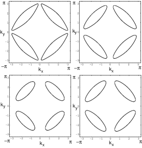
Figure 1: Contour plot of the hole pockets at the fixed value of the chemical potential $\mu=-0.36\;\text{eV}$ as the DDW gap is varied (implicitly as a function of doping $x$). Proceeding clockwise from the left panel on the top, $W_{0}(x)=0.01,0.05,0.1,0.15\;\text{eV}$; these numbers are for illustrative purposes only, and the $\mu$ was chosen so as to focus on the lower band only.

Before doing an explicit calculation, it is revealing to plot the hole pockets as the amplitude of the DDW gap $W_{0}(x)$ is increased for $\mu$ varying smoothly as a function of doping $x$, in particular we show the results for a fixed value of $\mu$ in Fig. 1. One can see that the hole pockets become less elliptical as $W_{0}$ is increased at constant $\mu$. So, even though $\mu$ is kept constant, with increasing $W_{0}$ below $x_{c}$, the curvature of the holepockets increases where the Fermi velocity is largest, Beaulac consequently $I_{xy}$ increases, and the perimeter decreases, so that $I_{xx}$ decreases. Beaulac The net result is an increase of $\omega_{H}$. This is a robust explanation of the increase of $\omega_{H}$ as the system is underdoped in agreement with Rigal et al.Rigal

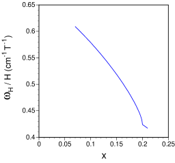
Figure 2: The Hall frequency ${\omega}_{H}$ as a function of $x$. The choices of the DDW gap amplitude and the chemical potential are described in the text.

To be quantitative, we explicitly calculate $\omega_{H}$ using Eq. (13) and the band structure parameters given above. Concomitantly, as mentioned above, $\mu$ was determined from the band structure. The results are shown in Fig. 2. The results are clearly consistent with the experiment of Rigal et al.Rigal The enhancement, as the system is underdoped, is significant, even though its actual magnitude is perhaps a factor of two smaller. Moreover, the absolute magnitudes are well captured. Beyond this, it is difficult to compare in detail. The experiment was performed on thin films of YBCO for which we do not have the precise knowledge of the doping levels, nor do we have a good criterion to relate the doping with the chemical potential. To complicate matters further, the chain contributions in YBCO are not included in our calculation, and these contributions were not subtracted in their experimental results. The parameters used here are generic; it is possible to improve the agreement with the experiment by adjusting them, but we do not find this to be a very meaningful exercise.

We then explore more closely the signature of the quantum critical point in the infrared Hall angle, which is already evident in Fig. 2. To demonstrate the robustness of the quantum critical point, we set $\mu$ to be a constant, equal to $-t=-0.3\;\text{eV}$ and use the mean field ansatz $W_{0}(x)=W_{0}(1-x/x_{c})^{1/2}$. For a representative value, we take $W_{0}=0.03\;\text{eV}$ and ${x_{c}}=0.2$. These are identical to our previous parametrizations.nHall The results are shown in Fig. 3.

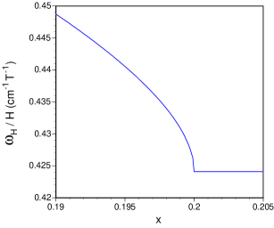
Figure 3: The Hall frequency ${\omega}_{H}$ close to the quantum critical point $x_{c}=0.2$, with $\mu$ set to a constant, equal to $-0.3$ eV.

By examining the integrals $I_{xy}$ and $I_{xx}$ in more detail, we find that, close to the critical doping, $\omega_{H}(x)=C_{1}+{C_{2}}{W_{0}}(x_{c}-x)^{1/2}$, where $C_{1}$ and $C_{2}$ are constants, and the slope diverges at the transition. (At finite temperature, this will be rounded.) We emphasize that although the hot spots determine the critical singularity close to $x_{c}$,nHall the increase of $\omega_{H}$ is determined by the evolution of the hole pockets and the gapping of the Fermi surface as the doping is decreased.

V Conclusion

The Hall angle measurements of Rigal, et al. Rigal are strong evidence for the existence of hole pockets in the underdoped cuprates. We believe that DDW order is the simplest explanation which is also consistent with the absence of hole pockets in ARPES. Consistency with both of these experiments (and the Hall number measurement of Ref. Boebinger, ) is a strong challenge of other proposals for the pseudogap. Our analysis opens a number of interesting directions for future research. Our calculation could be extended using the Kubo formalism, which would have a wider region of validity. A more careful comparison between theory and experiment could be made with a better model for the chemical potential at the precise doping levels of the experiment. Finally, further exploration of the putative quantum critical point at $x=x_{c}$ at which DDW order vanishes could more firmly establish its existence and its properties.

- (1) S. Chakravarty and H. -Y. Kee, Phys. Rev. B 61, 14821 (2000).
- (2) S. Chakravarty, R. B. Laughlin, D. K. Morr, and C. Nayak, Phys. Rev. B 63, 094503 (2001).
- (3) S. Tewari, H. -Y. Kee, C. Nayak, and S. Chakravarty , Phys. Rev. B 64, 224516 (2001).
- (4) S. Chakravarty, C. Nayak, S. Tewari, and X. Yang, Phys. Rev. Lett. 89, 277003 (2002).
- (5) K. Hamada and D. Yoshioka, Phys. Rev. B 67, 184503 (2003); S. Chakravarty, C. Nayak, and S. Tewari, Phys. Rev. B 68, 100504(R) (2003).
- (6) H. -Y. Kee and Y. B. Kim Phys. Rev. B 66, 012505 (2002).
- (7) S. Chakravarty, Phys. Rev. B 66, 224505 (2002).
- (8) H. -Y. Kee and Y. B. Kim, Phys. Rev. B 66, 052504 (2002).
- (9) S. Chakravarty, H. -Y. Kee, C. Nayak, Int. J. Mod. Phys. B 15, 2901 (2001).
- (10) S. Chakravarty, H. -Y. Kee, C. Nayak, in Physical Phenomena at High Magnetic Fields - IV, eds. G. Boebinger, Z. Fisk, L. P. Gorkov, A. Lacerda, J. R. Schrieffer (World Scientific, Singapore, 2002).
- (11) H. A. Mook, Pengcheng Dai, S. M. Hayden, A. Hiess, J. W. Lynn, S. -H. Lee, and F. Dogan, Phys. Rev. B 66, 144513 (2002).
- (12) S. Chakravarty, H. -Y. Kee and K. Voelker, Nature 428, 53 (2004).
- (13) L. B. Rigal, D. C. Schmadel, H. D. Drew, B. Maiorov, E. Osquigil, J. S. Preston, R. Hughes, G. D. Gu, cond-mat/0309108.
- (14) One might be concerned that our model is in contradiction with claims that the nodal fermi velocity is independent of doping in copper oxide superconductors [X. J. Zhou et al., Nature 423, 398 (2003)]. An incorrect, naive argument can be constructed to show that the Fermi velocity will vary as with doping for any model with hole pockets – thereby supposedly ruling out such models. If we assume that the hole pockets are circular, then it might be argued that the associated with the hole pocket will lead to the relation ; hence, the nodal Fermi velocity should be given by , assuming that the effective mass is unchanged. That this is simply an incorrect argument can be seen from Ref. ARPES, . It is trivially seen that, along the nodal direction, seen in ARPES is the same as that predicted by the band structure because of the special properties of the coherence factors.ARPES This is approximately true even away from this direction, as was verified by explicit calculations. In any case, we also do not find the experimental evidence of the doping independence of convincing: a collage of measurements of chemically diverse materials, in each of which has significant, but conflicting doping dependence, was used to argue that statistically there is no overall doping dependence. Finally, in the same experimental paper mentioned in this footnote, it was also argued that the ‘high-frequency Fermi velocity’ diverges as , as the doping . This is not a very meaningful statement, as at higher energies there are no quasiparticles to speak of in the ARPES spectra.
- (15) F. F. Balakirev, J. B. Betts, A. Migliori, S. Ono, Y. Ando, G. S. Boebinger, Nature 424, 912 (2003).
- (16) See, for example, J. M. Ziman, Electrons and phonons (Oxford University Press, Oxford, 1960).
- (17) R. Peierls, Surprises in Theoretical Physics (Princeton University Press, Princeton, 1979); see also J. Rammer and H. Smith, Rev. Mod. Phys. 58, 323 (1986).
- (18) See, for example, M. Tinkham, Introduction to superconductivity, 2nd. ed. (Mc-Graw-Hill, New York, 1996).
- (19) A. Carrington, A. P. Mackenzie, C. T. Lin, and J. R. Cooper, Phys. Rev. Lett. 69, 2855 (1992); H. Kontani, K. Kanki, and K. Ueda, Phys. Rev. B 59, 14723 (1999).
- (20) E. Abrahams and C. M. Varma, Phys. Rev. B 68, 094502 (2003)
- (21) K. Segawa and Y. Ando, Phys. Rev. Lett. 86, 4907 (2001).
- (22) Y. Ando, Y. Kurita, S. Komiya, S. Ono, and K. Segawa, preprint.
- (23) P. W. Anderson, Phys. Rev. Lett. 67, 2092 (1991); P. Coleman, A. Schofield, and A. M. Tsvelik, Phys. Rev. Lett. 76, 1324 (1996); G. Kotliar, A. Sengupta, and C. M. Varma, Phys. Rev. B 53, 3573 (1996).
- (24) See, for example, T. P. Beaulac, F. J. Pinski, and P. B. Allen, Phys. Rev. B 23, 3617 (1981).
- (25) It might be argued from the one-component analysis of optical measurements that for energies above the pseudogap scale [for a review, see D. B. Tanner and T. Timusk, in Physical properties of high temperature superconductors III, D. M. Ginsberg editor, (World Scientific, Singapore, 1992)], which is consistent with the marginal fermi liquid phenemenology.Abrahams We find that for underdoped materials, relevant to the present discussion, a better description may be in terms of a two-component analysis, as described in the same review article mentioned in this footnote. In a two-component analysis, where a Drude part and a mid-infrared part are separated out, there are no such restrictions on . The appropriateness of the two-component analysis in the underdoped regime has been emphasized recently [W. J. Padilla et al., preprint, submitted to Phys. Rev. Lett.]. Moreover, the Hall scattering rate and the transport scattering rate behave differently, as emphasized in Ref. Rigal, , and the former does not obey this inequality. These complications are beyond the scope of the present paper.
- (26) J. W. Loram, J. Luo, J. R. Cooper, W. Y. Liang, and J. L. Tallon, J. Phys. Chem. Solids 62, 59 (2001).