Breakup of a Stoner model for the 2D ferromagnetic quantum critical point

Abstract

Re-interpretation of the results by [A. V. Chubukov et. al., Phys. Rev. Lett. 90, 077002 (2003)] leads to the conclusion that ferromagnetic quantum critical point (FQCP) cannot be described by a Stoner model because of a strong interplay between the paramagnetic fluctuations and the Cooper channel, at least in two dimensions.

Recent experimental observations of superconductivity in a close proximity to the ferromagnetic quantum critical point (QCP) in a few itinerant ferromagnets such as heavy fermion compounds UGe₂ Saxena , URhGe Aoki and also in ZrZn₂ Pfleiderer have revived an interest to whether the magnetic fluctuations in the vicinity of ferromagnetic QCP provide a fundamental mechanism for the ”$p$-wave” superconductivity. The idea of the exchange by paramagnons turned out to be crucial for understanding the mechanism underlying the superfluid state in ³He at low temperatures Leggett . In a broader context, relevance of paramagnetic fluctuations to the appearance of superconductivity at the border of a magnetic transition has been discussed in Mathur and Joerg where reader will find the history of the problem and the comprehensive list of references.

Starting already with the one of the first papers on the subject Appel there were numerous efforts to evaluate the superconducting transition temperature mediated by strong paramagnetic fluctuations for both ferromagnetic and paramagnetic phases Bedell ; Millis ; Monthoux . Most of these results bear the numerical character, and this obscures the fact that there is, as we believe, some flaw in the very model. Most of the authors deal with the Stoner model where an instability of the paramagnetic itinerant state comes about with the increase of the on-site Hubbard interaction, $U$, that leads to the appearance of ferromagnetism. Variation in the value of the Stoner factor governs then changes in a value of the Curie temperature by varying an external parameter (in a more general form these ideas can be formulated in terms of the Fermi liquid theory Kondratenko by involving the Pomeranchuk instability Pomeranchuk ; Abrikosov ). Below we will try to demonstrate that such a model is not self-consistent, at least for the $2D$ systems.

The first question one faces while discussing any phase transition is how close one can approach the line of a transition. The problem of a singularity, or magnitude of fluctuations, looks simpler near the ferromagnetic QCP (the ending point of the phase diagram at $T=0$). The outcome of the analysis done by Hertz Hertz and recently by Millis Millis2 is that near such QCP fluctuations retain their mean field character due to an increase in effective dimensionality to account for an involvement of the frequency variable at zero temperature. We argue, that the hypothesis of the ferromagnetic QCP with the paramagnon propagator Hertz would lead to the developing of superconducting fluctuations at such a scale which breaks the validity of Hertz analysis far away from the vicinity of the imaginable QCP. In other words, a Stoner like ferromagnetic QCP is not self-consistent namely because it seemingly leads to such strong pairing fluctuations that make incorrect independent analysis of the spin ”zero sound” and Cooper channels. Below, we would like to prove our point by re-interpreting the results of the recent paper by Chubukov et al. Chubukov .

The emphasis in Ref. Chubukov has been put to demonstrate that superconducting transition near the ferromagnetic QCP may turn out to be of the first-order. The authors of Chubukov used the standard ansatz for the longitudinal fluctuations propagator Hertz . To get rid of the so-called non-adiabatic corrections and to reduce the gap equations to the well known form of the strong coupling ones (”Eliashberg” equations), the authors made an assumption that the interaction of electrons with the spin fluctuations is weak. A minor change below makes it more convenient to overview the physical picture of their model as a whole without resorting to numerical calculations.

Let us introduce the exchange part of interaction between the two electrons, $\widehat{I}({\mbox{\boldmath$r_{1}-r_{2}$}})$ as:

$$\widehat{I}({\mbox{\boldmath$r_{1}-r_{2}$}})=-I({\mbox{\boldmath$r_{1}-r_{2}$}})\left(\mbox{\boldmath$\widehat{\sigma}_{1}\cdot\widehat{\sigma}_{2}$}\right)$$ (1)

and assume that $\hat{I}({\mbox{\boldmath$r_{1}-r_{2}$}})$ has the ferromagnetic sign and bears a long-range character. After summing up all diagrams in the zero-sound channel the same way it was done in Hertz , one arrives to the following longitudinal spin-spin fluctuation propagator:

$$\widetilde{I}(\mbox{\boldmath$q$};\omega_{n})=\frac{I(\mbox{\boldmath$q$})}{1-2~{}\nu\left(\varepsilon_{F}\right)I(\mbox{\boldmath$q$})\left[1-a\frac{|\omega_{n}|}{v_{F}q}\right]},$$ (2)

where $I(\mbox{\boldmath$q$})$ is the Fourier component for the interaction (1), $w_{n}=\pi{T}(2n+1)$ is the Matsubara frequency, $\nu(\varepsilon_{F})$ is the density of states at the Fermi level and the value of $a$ depends on the dimensionality of the system: $a=\pi/2$ for 3D and $a=1$ for 2D.

Cancellation in the denominator of (2) at $q\to{0}$ and $\omega_{n}/v_{F}q\ll{1}$ leads to the Stoner criterion: $1-2~{}\nu(\varepsilon_{F})I(0)\to{0}$. The factor in the square brackets in denominator in (2) is nothing but the electron polarization operator $\Pi(\mbox{\boldmath$q$};\omega_{n})$:

$$\Pi(\mbox{\boldmath$q$};\omega_{n})=\frac{T}{(2\pi)^{d}}\sum\limits_{\Omega_{l}}\int{d^{d}\mbox{\boldmath$l$}}~{}G(\mbox{\boldmath$q+l$};\omega_{n}+\Omega_{l})\cdot{G}(\mbox{\boldmath$l$};\Omega_{l}).$$ (2’)

proportional to the generalized electron spin susceptibility and calculated at small enough $q$ in the limit $|\omega_{n}|\ll{v_{F}{q}}$ (at this relation $\omega_{n}$ and $q$ appear in all equations below). In the opposite limit $\Pi(\mbox{\boldmath$q$};\omega_{n})$ decreases to zero, and the Stoner like enhancement rapidly disappears at $\omega_{n}{\sim}v_{F}{q}$.

According to Hertz , Eq. (2) for the ferromagnetic fluctuations does not experience renormalization at $T=0$ and $1-2~{}\nu(\varepsilon_{F})I(0)\to{0}$. To agree the form of Eq. (2) with the similar expressions in Chubukov we assume that $I(q)$ rapidly decreases with an increase in $q$. To be more specific, we accept the following notation:

$$2I(q)\nu(\varepsilon_{F})\equiv{I_{0}}\exp\left[-q^{2}/(p_{F}\vartheta)^{2}\right],$$ (3)

where

$$\vartheta\equiv\left(R{p_{F}}\right)^{-1}\ll{1}$$ (4)

is the parameter sharing the long range character of (1), which in turn leads the small angle scattering to prevail in Eq. (2). The interaction (1) is isotropic in the spin space. It is straightforward to account in Eqs. (1,2) for the presence of the magnetic anisotropy Millis .

As it was first pointed out in Schrieffer , spin fluctuations produce two effects in case of the phonon-mediated ($s$ - wave) pairing: they add to renormalization of the electron self-energy and they provide the pair breaking mechanism for the $S=0$ Cooper pair. Pair breaking effects are basically the same even for a triplet ($S=1$) pairing, however, the exchange between two electrons by longitudinal paramagnetic fluctuations leads to the attractive interaction in the triplet $(S=1)$ channel. For the electron’s Green function in the paramagnetic phase, $G^{-1}(\mbox{\boldmath$p$};\omega_{n})=i\omega_{n}-\varepsilon(\mbox{\boldmath$p$})-\Sigma(\mbox{\boldmath$p$};\omega_{n})$, we write:

$$\Sigma(\mbox{\boldmath$p$};\omega_{n})=\frac{c}{(2\pi)^{d}}{T}\sum\limits_{\omega_{n^{\prime}}}\int{d^{d}\mbox{\boldmath$p_{1}$}}\widetilde{I}(\mbox{\boldmath$p-p_{1}$};\omega_{n}-\omega_{n^{\prime}})G(\mbox{\boldmath$p_{1}$};\omega_{n^{\prime}}),$$ (5)

where $d$ is the dimensionality of the problem, and the coefficient $c$ in (5) depends on whether the exchange is isotropic ($c=3$) or a strong magnetic anisotropy is present ($c=2$ for ”easy plane” and $c=1$ for ”easy axis”). For the sake of simplicity we take $c=1$ (”easy axis”) in order to avoid additional complications related to the possibility of a first-order superconducting transition.

The superconducting order parameter $\widehat{\Delta}_{\alpha\beta}(\mbox{\boldmath$p$};\omega_{n})$ is chosen below in the form:

$$\widehat{\Delta}_{\alpha\beta}(\mbox{\boldmath$p$};\omega_{n})=i\left[(\mbox{\boldmath$\widehat{\sigma}\cdot{d}$}(\mbox{\boldmath$p$};\omega_{n}))\widehat{\sigma}_{y}\right]_{\alpha\beta}$$ (6)

and near transition the vector $\mbox{\boldmath$d(p$};\omega_{n})$ satisfies the linear equation:

$$\mbox{\boldmath$d(p$};\omega_{n})=\frac{T}{(2\pi)^{d}}\int{d^{d}}\mbox{\boldmath$p_{1}$}\widetilde{I}(\mbox{\boldmath$p-p_{1}$};\omega_{n}-\omega_{n^{\prime}})~{}G(\mbox{\boldmath$p_{1}$};\omega_{n^{\prime}})~{}G(-\mbox{\boldmath$p_{1}$};-\omega_{n^{\prime}})\mbox{\boldmath$d(p_{1}$};\omega_{n^{\prime}})$$ (7)

which would serve to determine the dependence of the superconducting transition temperature on the proximity to the QCP in Eq. (2). According to Chubukov , the vicinity of the ferromagnetic QCP where onset of superconductivity acquires a non-perturbative character is much broader in 2D then in 3D. Consequently, our discussion will be restricted to the 2D situation only.

Let us express vector $q$ in Eq. (3) through the angle of scattering along the Fermi surface, $\varphi\ll{1}$:

$$\mbox{\boldmath$q$}^{2}={p_{F}}^{2}\varphi^{2}$$ (8)

In Eqs. (5,7) one can integrate over the energy variable component, $\xi_{1}=v_{F}(p_{1}-p_{F})$. Dependence on $\mid\mbox{\boldmath$p$}\mid$ in the order parameter $\widehat{\Delta}_{\alpha\beta}(\mbox{\boldmath$p$};\omega_{n})$ can be neglected because of smallness of the scattering angle, $\varphi$:

$$\mbox{\boldmath$d$}(\mbox{\boldmath$p$};\omega_{n})\Rightarrow\mbox{\boldmath$d$}(\omega_{n}).$$ (9)

Introducing the notation for proximity to the QCP

$$1-I_{0}=\tau\ll{1}$$ (10)

after simple calculation Eq. (7) acquires the form:

$$\mbox{\boldmath$d$}(\omega_{n})=T_{c}\sum\limits_{\omega_{n^{\prime}}=-\infty}^{\infty}\frac{i\pi\langle\widetilde{I}\rangle_{\omega_{n}-\omega_{n^{\prime}}}}{i\omega_{n^{\prime}}-\Sigma(\omega_{n^{\prime}})}\mbox{\boldmath$d$}(\omega_{n^{\prime}}),$$ (11)

where

$$\langle\widetilde{I}\rangle_{\omega}=\frac{\vartheta}{2\pi}\int\limits_{0}^{\infty}\frac{ds}{\tau+s^{2}+\frac{\omega}{v_{F}p_{F}}\frac{1}{s\vartheta}}$$ (12)

comes about after integrating (2) over $\varphi$ and making use of Eqs. (3,4,8) in the expansion:

$$1-2I(\mbox{\boldmath$q$})\nu(\varepsilon_{F})\simeq\tau+\left({\varphi}/{\vartheta}\right)^{2}$$ (13)

In equations above we have neglected all the vertex corrections to the bare vertices. With the help of the explicit expressions for $\widetilde{I}(\mbox{\boldmath$p$};\omega_{n})$, it will be easy to verify that the higher order corrections are small provided that our parameter $\vartheta$ above is small.

Figure 1: Vertex correction to the interaction. Dashed and solid lines are the paramagnon and fermionic propagators, respectively.

Straightforward calculation of the first vertex correction to the self-energy $\Sigma(\mbox{\boldmath$p$};\omega_{n})$ (5) shown in Fig. 1

$$\delta\Gamma^{(1)}=\frac{i\pi{T}}{2}\sum\limits_{\omega_{m}}\left[sign(\omega_{m}+\Omega_{l})-sign(\omega_{m})\right]\times$$

$$\int\limits_{0}^{\infty}\frac{d\varphi}{2\pi}\frac{1}{(\mbox{\boldmath$v$}_{F}\mbox{\boldmath$k$}-i\Omega_{l})(\tau+\varphi^{2}+\frac{\mid{\omega_{m}-\omega_{n}\mid}}{2\varepsilon_{F}\vartheta\varphi})}$$

gives the following order of magnitude estimate:

$$\delta\Gamma^{(1)}\sim\left({\vartheta}/{\sqrt{\tau}}\right)\cdot\left({\Omega_{l}}/{v_{F}k}\right)$$ (13’)

In notations (12) denominator in (11) is:

$$i\omega_{n}-\Sigma(\omega_{n})=i\omega_{n}+i\pi{T}\sum\limits_{\omega_{n^{\prime}}=-\omega_{n}}^{\omega_{n}}\langle\widetilde{I}\rangle_{\omega_{n^{\prime}}}$$ (14)

Substitution $s=z\sqrt{\tau}$ transforms (12) into:

$$\langle\widetilde{I}\rangle_{\omega}=\left(\frac{\vartheta}{2\pi\sqrt{\tau}}\right)\int\limits_{0}^{\infty}\frac{zdz}{z(1+z^{2})+\frac{\omega}{\omega_{0}}\left(\frac{\vartheta}{4\sqrt{\tau}}\right)^{3}}$$ (15)

with

$$\omega_{0}=\varepsilon_{F}\vartheta^{4}/32.$$ (16)

Frequency dependence in (12) serves as the cut-off:

$$\langle\widetilde{I}\rangle_{\omega}\approx{1}/{3\sqrt{3}}\left({\omega_{0}}/{\omega}\right)^{1/3}$$ (17)

for

$$\omega>\omega_{0}\left({4\sqrt{\tau}}/{\vartheta}\right)^{3}\simeq{2}\varepsilon_{F}\vartheta\tau^{3/2}$$ (17’)

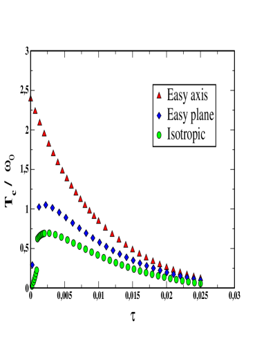
Figure 2: Numerical solution of Eq. (11) for $T_{c}$ as a function of $\tau$ for the various values of magnetic anisotropy constant, $c$ (see inset). Maximum in $T_{c}$ for easy plane and isotropic cases corresponds to the onset of the first-order transition into superconducting state.

Let us consider the paramagnetic phase ($\tau{>0}$) far enough from the QCP. Renormalization of the self-energy part $\Sigma(\omega_{n})$ is small, so that Eq. (11) converts into the weak-coupling problem:

$$1=\left(\frac{\theta}{4\sqrt{\tau}}\right)ln\left[\frac{\widetilde{\omega}}{T_{c}}\right],$$ (18)

where $\widetilde{\omega}$ is of the order of $\omega_{0}\left(\frac{4\sqrt{\tau}}{\vartheta}\right)^{3}$ (see Eq. (17’)). When $\sqrt{\tau}$ is further decreased, so it becomes comparable to $\vartheta$, the strong-coupling regime sets in with the cut-off frequency $\widetilde{\omega}\simeq\omega_{0}$ in (18). This leads to the new and important changes in $\Sigma(\omega)$. As it has already been discussed in Chubukov , one has the following asymptotic behavior of the self-energy part:

$$\Sigma(\omega)=\left\{\begin{array}[]{r@{\quad}}\omega\left({\vartheta}/{(4\sqrt{\tau})}\right),~{}~{}\omega\ll{2}\varepsilon_{F}\vartheta\tau^{3/2},\\ \left(\frac{3\sqrt{3}}{4}\varepsilon_{F}\vartheta^{4}\right)^{1/3}\cdot\omega^{2/3},~{}~{}\omega\gg{2}\varepsilon_{F}\vartheta\tau^{3/2}\end{array}\right.$$ (19)

The second asymptotic would signify appearance of the non-Fermi liquid regime in the close proximity to the QCP. It is seen, for fixed $\vartheta$, that the overall behavior of the critical temperature is defined by the value of the ”coupling” constant, $\lambda$:

$$\lambda={\vartheta}/{4\sqrt{\tau}}$$ (20)

As it is readily seen from Eq. (18), $T_{c}\sim\omega_{0}$ at $\lambda\sim{1}$.

Equation (11) for $T_{c}$ as a function of $\tau$ was solved numerically with the solution shown on Fig. 2. At $\tau\equiv{0}$ we obtain:

$$T_{c}\simeq{2.5\omega_{0}}\simeq{0.08\varepsilon_{F}\vartheta^{4}}.$$ (21)

Thus we conclude that $T_{c}$ is finite at $\tau=0$ and reaches the energy scale of the order of $\omega_{0}$ already at $\lambda\sim{1}$. The latter is also true for other cases shown on Fig. 2.

Let us therefore keep $\lambda\sim{1}$ and start gradually increasing value of the model parameter $\vartheta$. At $\vartheta\to{1}$ we should return back to the Stoner model with ordinary local interaction which is discussed in Hertz . We see from (13’), that non-adiabatic corrections remain of the order of one at $\lambda\sim{1},\vartheta\sim{1}$ and, hence, one expects that their exact treatment would not change qualitatively the estimate $T_{c}\sim\varepsilon_{F}$ from Eq. (21). On the other hand, at $\lambda\sim{1}$ and $\vartheta\to{1}$, $\tau=\vartheta^{2}/16\lambda^{2}\sim{1}$, and one cannot come close to QCP without forming a superconducting ground state, which in turn would change the polarization operator (2’). Obtaining such a high values for $T_{c}$ energetically so far away from the originally accepted position of the QCP ($\tau=0$) shows the intrinsic contradiction of the local Stoner model Hertz . At such a high energy scale the assumed proximity to a ”QCP” seems to be irrelevant for physical properties of the system. Mathematically, large $T_{c}\sim{\varepsilon_{F}}$ or/and large $\Delta$ lead to the change in the polarization operator Eq. (2’) to account for an interplay between the zero-sound and superconducting channels. The polarization operator (2’) is modified due to the presence of anomalous Gor’kov functions $F,F^{\dagger}$ in superconducting state at $T=0$. For $\vartheta\sim{1}$ and $\Delta\sim{T_{c}}\sim\varepsilon_{F}$ this introduces such a change in polarization operator that significantly reduces cancellation in the Stoner factor.

Remember now that at $\omega=0$ and $v_{F}q\to{0}$ expression (2’) used to describe a behavior of magnetic susceptibility near a ferromagnetic QCP. Similarly, modified polarization operator is proportional to electronic susceptibility in superconducting state. The latter would not go to zero at $T=0$ as it does for the $s$-wave pairing, even though it does not equal to normal susceptibility neither in any triplet state. The Stoner cancellation does not occur. Therefore, once superconductivity (18) arises at $\tau>0$ in the framework of the model with $\vartheta\ll{1}$, at $T=0$ the ground superconducting state as a function of external parameter continues to be stable while entering into the ferromagnetic state $(\tau<0)$ well beyond ”QCP”. This suggests a first order like phase competition between superconductivity and ferromagnetism at low temperatures.

All that has been said above poses a few questions. First, numerical calculations (see Ref. Bedell ; Millis ; Monthoux ) for $T_{c}$ making use of an exchange by longitudinal spin fluctuations give rather low values of critical temperature compared to the values of the bandwidth or the Fermi energy without special assumption of small angle scattering (the authors have been solving basically the same equations, i.e. no vertex corrections have been included). We believe, this is a result of some numerical smallness, such as the factor $1/32$ in Eq. (16). This smallness may restore QCP within some vicinity. Indeed, the low values of $T_{c}$ has been experimentally observed in a number of systems among which are Sr₂RuO₄, URhGe or ³He. In addition, in 3D the strong coupling regime of the above model sets on only in very close proximity to the QCP Chubukov . Note that the model itself does not determine the spatial symmetry of the triplet Copper pair wave-function: exchange by paramagnons is not the only interaction between the electrons in the Cooper channel. Thus, the paramagnon contribution in our model comes together with other interactions, $\Gamma_{l}\sim{1}$:

$$(3D):~{}-\vartheta^{2}|{ln(\tau)}|+\Gamma_{l};~{}~{}(2D):~{}-\frac{\vartheta}{\sqrt{\tau}}+\Gamma_{l},$$ (22)

where $\Gamma_{l}$ may be positive (here $\Gamma_{l}$ is a proper harmonics designed by the exact symmetry of the superconducting pairing). Onset of attraction in (22) takes place closer to $\tau=0$ and an effective interaction (22) remains reasonably weak ($\sim{1}$) in its vicinity  NotaBene .

To summarize, we have shown that competition with the superconductivity channel makes the Stoner model for ferromagnetic quantum critical point not self-consistent. FQCP can be realized only due to the presence of a numerically small parameter or other repulsive interactions in the triplet channel that weaken the attraction mediated by paramagnons, at least in 2D.

The authors thank A. Chubukov, A. Finkel’stein and D. Morr for fruitful discussions.

This work was supported by DARPA through the Naval Research Laboratory Grant No. N00173-00-1-6005 (M.D.) and by the NHMFL through the NSF cooperative agreement DMR-9527035 and the State of Florida (L.P.G.).

References

- (1) S. S. Saxena et al., Nature 394, 39 (1998).
- (2) D. Aoki et al., Nature 413, 61 (2001).
- (3) C. Pfleiderer et al., Nature 412, 58 (2001).
- (4) A. J. Leggett, Rev. Mod. Phys. 47, 331 (1975).
- (5) N. D. Mathur et al., Nature 394, 39 (1998).
- (6) A. Chubukov, D. Pines and J. Schmalian, in The Physics of Conventional and Unconventional Superconductors, ed. by K.H. Bennemann and J.B. Ketterson (Springer-Verlag, 2002)
- (7) D. Fay and J. Appel, Phys. Rev. B 22, 3173 (1980).
- (8) Z. Wang, W. Mao, and K. Bedell, Phys. Rev. Lett. 87, 257001 (2001); K. B. Blagoev, J. R. Engelbrecht, and K. Bedell, Phys. Rev. Lett. 82, 133 (1999).
- (9) R. Roussev and A. J. Millis, Phys. Rev. B 63, 140504 (2001).
- (10) Ph. Monthoux and G. G. Lonzarich, Phys. Rev. B 59, 14598 (1999).
- (11) I. E. Dzyaloshinskii and P. S. Kondratenko, Sov. Phys. JETP 43, 1036 (1976).
- (12) I. Ia. Pomeranchuk, Sov. Phys. JETP Lett. 8, 361 (1959).
- (13) A. A. Abrikosov and I. E. Dzyaloshinskii, Sov. Phys. JETP 35, 535 (1959).
- (14) J. Hertz, Phys. Rev. B 14, 1165 (1976).
- (15) A. J. Millis, Phys. Rev. B 48, 7183 (1993).
- (16) A. V. Chubukov, A. M. Finkel’stein, R. Haslinger, and D. Morr, Phys. Rev. Lett. 90, 077002 (2003).
- (17) N. F. Berk and J. R. Schrieffer, Phys. Rev. Lett. 17, 433 (1966).
- (18) adding breaks the logarithmic self-consistance due to the form of the kernel (17) and the self-energy part (14). Non-zero in (22) narrows the vicinity of QCP where solutions for shown on Fig. 2 apply.