Universality in the Screening Cloud of Dislocations Surrounding a Disclination

Abstract

A detailed analytical and numerical analysis for the dislocation cloud surrounding a disclination is presented. The analytical results show that the combined system behaves as a single disclination with an effective fractional charge which can be computed from the properties of the grain boundaries forming the dislocation cloud. Expressions are also given when the crystal is subjected to an external two-dimensional pressure. The analytical results are generalized to a scaling form for the energy which up to core energies is given by the Young modulus of the crystal times a universal function. The accuracy of the universality hypothesis is numerically checked to high accuracy. The numerical approach, based on a generalization from previous work by S. Seung and D.R. Nelson (Phys. Rev A 38:1005 (1988)), is interesting on its own and allows to compute the energy for an arbitrary distribution of defects, on an arbitrary geometry with an arbitrary elastic energy with very minor additional computational effort. Some implications for recent experimental, computational and theoretical work are also discussed.

1 Introduction

Topological defects, mainly disclinations and dislocations, play a crucial role in the understanding of the physics of many two-dimensional (2D) systems [1]. Although computational techniques such as analytical methods, Ewald summation techniques [2], Monte Carlo simulations [3], etc.. can be used in many different contexts, they become quite inefficient in other situations, particularly with crystals having a boundary or lying on a curved background. In this paper, a new approach based on previous work by Seung and Nelson [4] will be discussed in detail. The computational methods developed allow to obtain the lowest energy configuration for an arbitrary distribution of defects in a crystal lying on an arbitrary geometry with an arbitrary elastic energy at zero temperature. The method is general enough to include Bravais lattices other than the triangular case. A discussion of the screening cloud of dislocations surrounding a disclination will be presented. This problem will be used as a testing ground where the results may be compared with the analytical predictions from elasticity theory derived in this paper.

An interesting experimental example where the dislocation cloud surrounding a disclination appear is given by colloidal particles crystallizing on the surface of a sphere (colloidosomes) [5]. As a consequence of the Euler theorem [6], an sphere must have a total disclination charge of 12. If the total number of particles forming the sphere is large enough, the ground state contains more defects than the 12 necessary to satisfy the Euler theorem. Those additional defects are dislocations surrounding a disclination, as illustrated in fig. 1, arranging in the form of grain boundaries. Those grain boundaries have two very distinctive features 1) terminate inside the medium and 2) have a total disclination charge of +1. These features are intimately related to the geometry of the problem and should appear whenever the Gaussian curvature is large enough [7, 8, 9]. Similar structures have been also observed in simulations of the Thomson problem [10, 11, 12]. Clouds of dislocations (with the minus disclinations playing the role of plus charges) should also appear in crystals on a negatively curved background [13]. Those situations are relevant as two dimensional analogs of the frustration associated with the three dimensional tetrahedral packing [14] and other surface physics problems [15, 16].

The problem of grain boundaries radiating out of disclinations is also important for understanding certain aspects of the problem of two-dimensional melting. The KTHNY [17, 18, 19] scenario predicts a two stage melting from a crystal into an isotropic phase via an hexatic phase. This picture has been confirmed by a large number of examples (see [20, 3] for reviews). Very precise numerical simulations [21] have found very good agreement with the predictions of the KTHNY scenario. Different inherent structures (IS) characterize each phase, and disclinations appear as forming grain boundaries with very similar characteristics as the ones found in the Colloidosome problem. Similar structures have been found in recent simulations, and the defects have been characterized by $1/f$ noise [22]. Recent experiments on plasmas [23] and colloids [24, 25], have found also a similar situation, with correlation functions in good agreement with the KTHNY scenario and grain boundaries with similar characteristics. Alternative melting scenarios have exploited the short-range nature of the stresses produced by grain boundaries of dislocations [26].

The physics of Langmuir monolayers has received a lot of attention in recent years [27, 28], but many important questions have not yet been clarified. It seems very clear that topological defects play a crucial role in problems such as melting or the collapse of monolayers [29]. More sophisitcated systems, such as sphingomyelin, where additional hydrogen bonding may be formed, show a much richer phase diagram [30]. Biphasic surfactant monolayers show additional defect structures (mesas) [31].

Radial grain boundaries radiating from a central disclination are also found in hexatic $I^{*}$ and crystal $J^{*}$ tilted liquid crystal phases [32]. The tilt is used to force a disclination and a pattern of radial grain boundaries (with 5 arms) is observed.

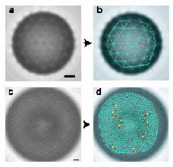
Figure 1: Ground state configurations for a large and small colloidosome. For a large colloidosome, finite length grain boundaries radiate out of the disclination (from [5]).

The methods described in this paper are also relevant for a restricted type of quantum dots [33] in which the density of electrons is is small and the external disorder potential is weak enough so that the electrons in the dot form a Wigner crystal, so called “Wigner Crystal Islands” [34]. The methods presented in this paper are relevant to this case as well, as only a change of the boundary conditions for the problem is required.

Dislocation clouds also appear in many other problems such as, partially polymerized membranes [35, 36], Wigner crystals [37] and in carbon nanotubes, particularly in the so called “Onion” rings, which are successive spherical layers of graphite [38].

The organization of the paper is as follows. A review of continuum results is given in Sect. 2. The discretized approach is introduced in sect. 3 and compared against the continuum results for isolated defects. The scaling relations satisfied by the energy are derived in sect. 4. Numerical results are presented in sect. 5 and their universality with respect to the Lame coefficients is discussed in sect. 6. Sect 7 is a brief overview of the effect of curvature. We wrap up with some conclusions in sect. 8. Several technicalities are relegated to the appendices.

2 Continuum Results

The elastic energy of a continuum is given by [39]

$$F=\frac{1}{2}\int d^{2}r(2\mu u^{2}_{\alpha\beta}+\lambda(u_{\alpha\alpha})^{2})$$ (1)

where the strain tensor is defined as

$$u_{\alpha\beta}=\frac{1}{2}(\frac{\partial{u_{\alpha}}}{\partial{x_{\beta}}}+\frac{\partial{u_{\beta}}}{\partial{x_{\alpha}}}+\frac{\partial{u_{\rho}}}{\partial{x_{\beta}}}\frac{\partial{u_{\rho}}}{\partial{x_{\alpha}}})\ .$$ (2)

The quadratic term in the strain tensor is usually dropped, as it usually amounts to higher order negligible corrections to the total energy. Those terms cannot be entirely neglected if disclinations are involved [4] (For consistency, other energy terms quadratic in the strain tensor should also be included, but for the sake of simplicity this point will be ignored). The Young modulus and Poisson ratio are

$$K_{0} = 4\mu\frac{\mu+\lambda}{2\mu+\lambda}$$

$$\nu = \frac{\lambda}{2\mu+\lambda}.$$ (3)

Using known analytical techniques, the strains for a dislocation and a disclination may be solved in linear order [39, 4]. For a dislocation with Burgers vector ${\bf b}=b{\bf e}_{x}$ the result is [39]

$$u_{x} = \frac{b}{2\pi}(\phi+\frac{K_{0}}{8\mu}\sin(2\phi))$$ (4)

$$u_{y} = -\frac{b}{2\pi}(\frac{\mu}{\lambda+2\mu}\log(r/a)+\frac{K_{0}}{8\mu}\cos(2\phi)).$$

The strains for disclinations of charge $s$ are [4]

$$u_{r} = -\frac{s}{2\pi}r(1-\frac{2\mu}{2\mu-\lambda}(A_{s}+1/2)-\frac{2\mu}{2\mu+\lambda}\log(r/R))$$

$$u_{\phi} = \frac{s}{2\pi}r\phi\ ,$$ (5)

There is an arbitrary constant $A_{s}$ which will be determined in the appendix sect. A.

Plugging Eq. 4 and Eq. 2 into Eq. 1 The energies for a dislocation of Burgers vector $b$ is

$$F=\frac{|{\bf b}|^{2}}{8\pi}K_{0}(\ln(R/a)+\mbox{const}).$$ (6)

As it is shown in the appendix sect. A, the constant $A_{s}$ is related to the two-dimensional pressure $\Pi$. Following the same steps as for a dislocation, the energy for an isolated disclination of charge $s=\frac{\pi}{3}q_{i}$ under pressure becomes

$$F=\frac{s^{2}}{32\pi}K_{0}R^{2}+\frac{\pi\Pi^{2}}{8{\cal B}}R^{2}\ .$$ (7)

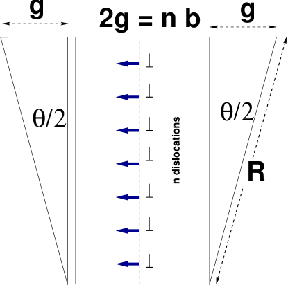
Figure 2: Relation between the aperture angle $\theta$ of a grain boundary of dislocations and its total Burgess vector $nb$ and radius of the crystal $R$.

The energy dependence, growing as $R^{2}$, is energetically very costly. Grain boundaries of dislocations may screen out the disclinations, thus reducing the huge energy cost of an isolated disclination, if the angle of the grain boundary exactly compensates the missing or additional wedge (a multiple of $\frac{\pi}{3}$ for triangular lattice) caused by the disclination. From the geometric argument in fig. 2, the angle of grain boundary $\theta$ is given by

$$2R\sin(\theta/2)=nb,$$ (8)

where $n$ is the total number of dislocations all having Burgers vector $b$. Further assuming a constant spacing of dislocations within the grain $D$, the relation $B=Rb/D$ holds and one gets

$$2\sin(\theta/2)=b/D.$$ (9)

upon identifying $\theta$ with the missing or additional wedge removed to form the disclination [9], Eq. 9 becomes

$$2\sin(\frac{\pi}{6m})=b/D\ ,$$ (10)

leading to an equation for the spacing $D$ as a function of the number of arms $m$. A detailed analytical proof for this result using linear elasticity theory is provided in appendix B, where the total energy of the system of a disclination and an m-arm grain boundary (see fig. 5) is given by Eq. 53. There is also a linear term in $R$ arising from two different contributions, the stresses of grain boundaries of dislocations, discussed in appendix C and the core energies of the defects. The total contribution to the energy is then,

$$F=\frac{(s-m\frac{b}{D})^{2}}{32\pi}K_{0}R^{2}+\left(H(2\pi\frac{a}{D})+4\pi c\right)m\frac{K_{0}}{4\pi}\frac{a^{2}}{D}R\ ,$$ (11)

where the function $H$ is defined in the appendix Eq. 57. The pressure $\Pi$ has been set to zero. The total number of dislocations is $n=m\frac{R}{D}$. The core energy has been parametrized as $E_{core}=K_{0}a^{2}c$, where $c$ is a dimensionless coefficient (but not independent of the elastic constants).

If the spacing $D$ is given by Eq. 10, the leading $R^{2}$ term in Eq. 11 is canceled and only the linear term in $R$ , which we denote as $f$, survives

$$f\equiv\left(H(2\pi\frac{a}{D})+4\pi c\right)m\frac{K_{0}}{4\pi}\frac{a^{2}}{D}R\ ,$$ (12)

For future reference, we quote the result for large $m$

$$f=\left(\frac{1}{4\pi}(1-\log(\frac{2\pi^{2}}{3m}))+c\right)mK_{0}a^{2}\frac{R}{D}\ .$$ (13)

At perfect screening $m\frac{a}{D}=q_{i}\frac{\pi}{3}$ and the energy grows logarithmically with $m$. All previous results assume an infinite system (large $R$). How large $R$ must be in order that the infinite radius result hold, will be estimated next.

The interaction energy of two grain boundaries decays exponentially fast as a function of their mutual distance [40], with a decay length

$$\lambda_{gb}=\frac{D}{2\pi},$$ (14)

$D$ being the distance between dislocations within the grain (fig. 2).

dislocations that are a distance $L$ from the disclination will be invisible to the dislocations in other arms if

$$2L\sin(\pi/m)>>2\lambda_{g}\ .$$ (15)

therefore from Eq. 14 and Eq. 10 it follows

$$L>>\frac{3}{\pi}m^{2}b.$$ (16)

For $R>L$ the infinite result Eq. 12 will hold. The dependence of Eq. 16 on $m^{2}$ points out that the behavior Eq. 12 for large number of arms will not be reached until the radius $R$ is very large.

3 Discretization of the Elastic Free Energy

We consider a 2d triangular lattice of monomers with lattice constant $a$. The actual position of the $(n,m)$ monomer is described by ${\bf r}_{(n,m)}$ and it may be decomposed as

$${\bf r}_{(n,m)}=n{\bf e}_{1}+m{\bf e}_{2}+{\bf u}_{(n,m)}\ ,$$ (17)

where ${\bf u}_{b}$ is the strain at point $b$ and ${\bf e}_{i},i=1,2$ define a basis of the Bravais lattice. For a triangular lattice it is

$${\bf e}_{1} = {\bf e}_{x}$$ (18)

$${\bf e}_{2} = \frac{1}{2}{\bf e}_{x}+\frac{\sqrt{3}}{2}{\bf e}_{y}\ .$$

The discrete elastic free energy that we will use is

$$F=\frac{\epsilon}{2}\sum_{<bc>}(|{\bf r}_{bc}|-1)^{2}+\sigma\sum_{b,c}(\frac{1}{2}-\frac{{\bf r}_{bc}\cdot{\bf r}_{bc+1}}{|\bf{r}_{bc}||{\bf r}_{bc+1}|})^{2}\ .$$ (19)

The summation in the first term runs over links defined by vertices $a,b$, and in the second term the sum runs over all nearest neighbors of point $b$. Other discretizations are also possible but do not modify the results as it will be discussed.

In order to proof the equivalence of Eq. 19 with the continuum result Eq. 1, one must define the discrete derivatives first. The derivatives of a general function $f({\bf r})$ are only defined along the discrete direction of the triangular lattice, so a general derivative is precisely defined from

$$\partial_{x}f({\bf r}_{b}) = \frac{f({\bf r}_{b}+a{\bf e}_{1})-f({\bf r}_{b})}{a}$$ (20)

$$\partial_{y}f({\bf r}_{b}) = \frac{f({\bf r}_{b}+a{\bf e}_{2})-f({\bf r}_{b})-\frac{1}{2}(f({\bf r}_{b}+a{\bf e}_{1})-f({\bf r}_{b}))}{a\sqrt{3}/2}\ .$$

Using the previous definition, the discrete metric becomes

$$g_{ij}(b)=\partial_{i}{\bf r}_{b}\partial_{j}{\bf r}_{b}\ .$$ (21)

The distance between two nearest neighbor points is

$$|{\bf r}_{a}-{\bf r_{b}}|=(1+2u_{ij}e^{i}_{ab}e^{j}_{ab})^{1/2}\ ,$$ (22)

where the discrete strain tensor is defined from the derivatives Eq. 20 by

$$u_{\alpha\beta}=\frac{1}{2}(\frac{\partial{u_{\alpha}}}{\partial{x_{\beta}}}+\frac{\partial{u_{\beta}}}{\partial{x_{\alpha}}}+\frac{\partial{u_{\rho}}}{\partial{x_{\beta}}}\frac{\partial{u_{\rho}}}{\partial{x_{\alpha}}})\ .$$ (23)

Expanding Eq. 22 using Eq. 59 derived in the appendix, the first term of the discrete energy is identical to Eq. 1 with

$$\lambda = \frac{\sqrt{3}}{4}\epsilon$$

$$\mu = \frac{\sqrt{3}}{4}\epsilon\ .$$ (24)

The same expansion to the second term using the relations Eq. 60, 61, 62 from the appendix lead to

$$\lambda = 9\frac{\sqrt{3}}{4}\sigma$$

$$\mu = -9\frac{\sqrt{3}}{4}\epsilon\ .$$ (25)

The elastic constants of the two terms combined are then

$$\lambda = \frac{\sqrt{3}}{4}(\epsilon+9\sigma)$$

$$\mu = \frac{\sqrt{3}}{4}(\epsilon-9\sigma)\ ,$$ (26)

and therefore, Eq. 19 provides a suitable discretization of Eq. 1 with arbitrary elastic constants. It should be recalled that higher order terms in the displacement are dropped to lead to Eq. 3.

In this paper, the particular geometry that will be used consists of a plus or minus disclination (a pentagon or an heptagon respectively) at the center of the crystal. The total number of monomers forming the crystal is a function of the linear size $R$ and depends on the total number of dislocations. If only a center defect of charge $q_{i}$ is present, the total number of monomers is

$$M=(6-q_{i})\frac{R^{2}+R}{2}+1\ ,$$ (27)

Even with additional dislocations, the total number of points will still grow like $(6-q_{i})R^{2}$.

3.1 Energies of single defects

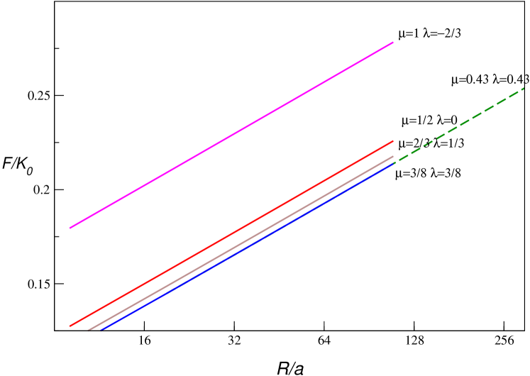
Figure 3: Results for the energy of an isolated dislocation as function of R for different values of the elastic constants.

The energies of isolated dislocations and disclinations will be compared against the analytical predictions derived previously. This will provide a benchmark to the present approach.

In fig. 3 the minimum energy results of a configuration containing a dislocation for different values of the Lame coefficients. A fit to the form of Eq. 6 yields

$$\frac{F}{K_{0}|{\bf b}|^{2}}=0.0395(2)\log(r)$$ (28)

in agreement within of $1\%$ with the analytical result $\frac{1}{8\pi}=0.03979$. The small deviation may be attributed to the neglect of higher order terms in the continuum calculation. Core energies may be computed from the intercept in fig 3. The results are summarized in table 1. It should be noted that core energies for crystals with the same Young modulus are different.

$(\mu,\lambda)$ $(1,-\frac{2}{3})$ $(\frac{1}{2},0)$ $(\frac{2}{3},\frac{1}{3})$ $(\frac{3}{8},\frac{3}{8})$ $(\frac{\sqrt{3}}{4},\frac{\sqrt{3}}{4})$ $\frac{E_{core}}{K_{0}a^{2}}$ $0.092(1)$ $0.042(1)$ $0.039(1)$ $0.029(1)$ $0.0285(1)$

Table 1: Core energies of dislocations as a function of Lame coefficients $(\mu,\lambda)$

The results of the same analysis for single disclinations are shown in table 2. The most accurate determination yields

$$\frac{F}{R^{2}K_{0}s^{2}}=0.00785(1)\ ,$$ (29)

both for plus and minus disclinations (Results for $\lambda=\mu$ were first obtained with less accuracy by [4]). Although the coefficient is off from the analytical result Eq. 7 by a significant amount, it is remarkably universal as a function of the elastic constants. The energies are also the same for both plus and minus disclinations within a $0.1\%$ accuracy (more accurate results do show that sevenfold defects have a marginally lower energy). There is, however, a term that grows linearly with $R$ in the discretized energy. This term is quoted also in table 2.

Figure 4: Plot of function $E(r_{b})$ describing the relative difference of the analytical solution and the numerical result.

$s$ $(1,-\frac{2}{3})$ $(\frac{1}{2},0)$ $(\frac{2}{3},\frac{1}{3})$ $(\frac{3}{8},\frac{3}{8})$ $R^{2}(+)$ $0.80(1)$ $0.79(1)$ $0.078(1)$ $0.0785(1)$ $R^{2}(-)$ $0.79(1)$ $0.78(1)$ $0.079(1)$ $0.0785(1)$ $R(+)$ $-0.003(1)$ $0.006(1)$ $0.007(1)$ $0.08(1)$ $R(-)$ $-$ $0.007(1)$ $0.008(1)$ $0.009(1)$

Table 2: Coefficient (Eq. 29) as a function of the Lame coefficients $(\mu,\lambda)$

It is also instructive to compare the continuum strain solution ${\bf r}_{A}$ Eq. 2 with the configuration from the discrete calculation. The difference will be quantified from the function

$$E(r_{b})=\frac{|{\bf r}_{b}-{\bf r}_{A}|}{|{\bf r}_{b}|+|{\bf r}_{A}|}$$ (30)

and it is plotted in fig. 4. The relative error is always below $0.01\%$, becoming as low as $10^{-6}\%$.

4 Scaling Relations for Grain Boundaries

The degrees of freedom defining a grain boundary of dislocations are (see fig. 5):

• $m$: number of arms.

• $l_{gb}$: Length of the grain boundary from the central disclination.

• $\Psi$: angle of the grain with some specified crystallographic axis.

• $D$: spacing of dislocations within each grain.

The spacing $D$ does not generally need to be restricted to be constant. The linear size of the system is $R$.

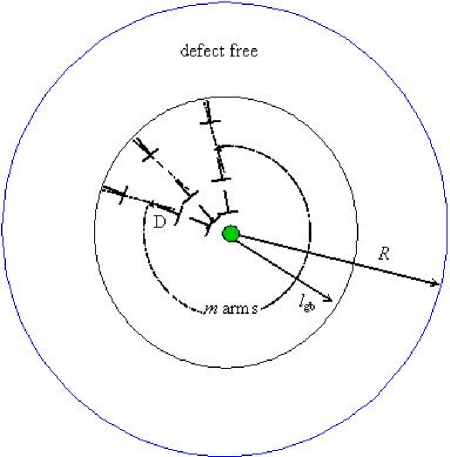
Figure 5: Degrees of freedom of a grain boundary.

It is convenient to define the dimensionless variable

$$x=l_{gb}/R\ ,$$ (31)

which by definition satisfies $0\leq x\leq 1$. $x=1$ implies that grains reach the boundary while $x=0$ implies no dislocations. Eq. 11 will be generalized (for zero temperature) by assuming that for intermediate values of $x$ the following scaling behavior holds

$$E=K_{0}R^{2}{\cal Q}(x,m,D,\Psi)$$ (32)

where as $x\rightarrow 0$ ${\cal Q}$ approaches Eq. 7. This scaling law however, may break down if the sub-leading linear terms in $R$ become comparable. The condition expressing this situation is given by (see Eq. 12).

$${\cal Q}(x_{c})\sim\frac{\pi x_{c}}{3R}f\ ,$$ (33)

If the term square in $R$ vanishes, this equation must hold for some $x_{c}$ and scaling will break down for all $x>x_{c}$.

If the square term in $R$ does not cancel, then the scaling relation must hold for large $R$ as well. That will be the case for spacings $D$ not satisfying Eq. 10. The ${\cal Q}$ function should exhibit a minima roughly at the critical $x_{m}$ where the additional angle added by the dislocations compensates the missing or additional angle by the disclinations. The critical $x_{m}$ is given by

$$x_{m}=2D\sin(\pi/(6m))\ ,$$ (34)

with the additional constraint $x_{m}<1$. Therefore the ${\cal Q}$ should exhibit a minima for $x_{m}$.

The angle $\Psi$, defined as the angle of the grain with respect a crystallographic axis, for an m-grain boundary commensurate with the p-fold symmetry of the central disclination will be constrained to

$$0\leq\Psi<\frac{\pi}{m}\ .$$ (35)

A straight-forward analytical calculation shows that ${\cal Q}$ should be independent of $\Psi$. It will be shown that this result ignores the constraints imposed on the Burgers vector by the underlying lattice.

5 Numerical study of grain Boundaries

5.1 Some computational details

The calculations have been done by relaxing an initial configuration consistent with the given distribution of defects using the conjugate gradient method. The numerical accuracy was tested by checking the convergence of the final results as a function of the tolerance error in the algorithm. Whenever different initial configurations consistent with the given distributions of defects were tried, the final result was found to be identical. The energies were computed to a seven digit precision or more.

For each value of the parameters, results were obtained for linear sizes ranging from $R=10$ to $R=200$ corresponding to typical volume sizes from $247$ to $140000$ monomers. Those lattices are, in many cases, larger than some experimental systems available. Free boundary conditions were incorporated by allowing the system to reach its natural extend without any external constraint.

The code has been written in C++ using objected oriented design. This provides the flexibility of incorporating any potentially new geometry, distribution of defects or discretization energy at any future time with a very minute effort. The code has some limitations too, one of them being that non-integer spacings (cases were dislocations within the grain should be slightly non-constant to mimic fractions of the lattice spacing) have not been implemented effectively. Typical minimizations of a system with $R=100$ (total number of monomers $M=25000$) take 9 minutes at a $10^{-10}$ precision and 5 minutes at $10^{-5}$ precision in a Dell 1.80 GHz dual Xeon procesor running Linux Red Hat. Further computational details will be presented elsewhere.

5.2 Scaling as a function of $l_{gb}$ and $D$

A plus disclination will be placed at the center of the crystal and grain boundaries will be fixed to have angle $\Psi=\pi/5$ and number of arms $m=5$. The energy will be investigated as a function of the parameters $l_{gb}$ and $D$. The elastic constants will be chosen as $\lambda=\mu$.

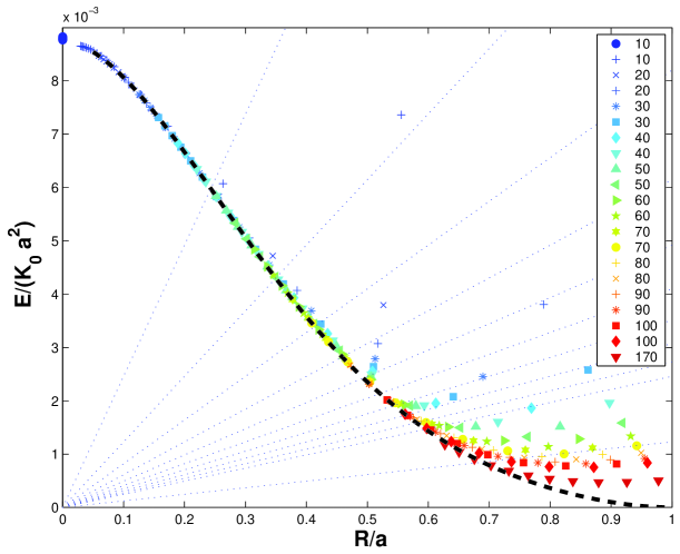
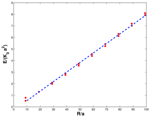
Figure 6: Plot of the scaling function Eq. 32 for $D=5$, $m=5$, $\Psi=\pi/5$ and sizes $R=10-170$. The dashed line is a fit with an extrapolation to $x->1$. The straight lines provide a visual solution to Eq. 33 and an estimate of the critical $x_{c}$ as a function of $R$.

Figure 7: Plot of the fit Eq. 12 to the results for $R\sim l_{gb}$.

The energy of relaxed configurations is plotted in fig. 7 as a function of the scaling variables. the ${\cal Q}$ function is plotted for a plus-disclination and a $m=5$ grain boundary with spacing $D=5$. The plots follow very well the ansatz in Eq. 32, with obvious deviations for values of $x$ closer to 1.

In order to determine the coefficient of the linear term in R, defined as $f$ in Eq. 12, it will be assumed that the points on fig. 7 for $x\sim 1$, which clearly do not scale, are described by Eq. 12. The results are plotted in fig. 7 and one obtains for the $f$-coefficient

$$f=0.081(5)\ .$$ (36)

Since we are not looking for a high precision value for the $f$-coefficient, two values for $l_{gb}$ were included for any given $R$. This provides strong evidence of the robustness of the fit. The theoretical value of the $f$ coefficient arises from a grain boundary contribution Eq. 56 and a core energy which may be estimated from a single dislocation (given in table 1). The two contributions give

$$f=0.063\mbox{(Grain Boundary)}+0.029\mbox{(Core Energy)}=0.092\ ,$$ (37)

considering the approximations involved (basically linear elasticity theory and non-interacting grains), the agreement with Eq. 36 is acceptable.

The value obtained for $f$ may be cross-checked by assuming that the scaling behavior will break down when the value for the linear term is, say one third, of the square term. The intersection of the straight lines in fig. 7 provide a visual solution to Eq. 33 and an estimate of the critical $x_{c}$ as a function of $R$ in reasonable self-consistent agreement, particularly for large values of $R$.

Three regions may be clearly identified from fig. 7:

• ($x\sim 0$): The energy is dominated by the strains of the central disclination and the effect of adding additional defects is negligible.

• ($0<<x<x_{c}$): The inclusion of more defects dramatically lowers the energy.

• ($x>x_{c}$): The core energy contribution sets in and scaling breaks down, the energy grows linearly with $R$, as apparent from fig. 7.

It should be noted from fig. 7 that if the intermediate region could be extrapolated to to $x\sim 1$ before the core energy terms would become noticeable, the energy would go to zero as $(x-1)^{2}$, that is, independent of the linear size $R$.

A typical relaxed final configuration is shown in fig. 13. The plot is only for a small region around the central disclination, but it clearly shows that for regions away of the defects the triangles forming the crystal are almost equilateral (unstrained).

5.3 Scaling function for non-optimal $D$ values at fixed $m$ and $\Psi$

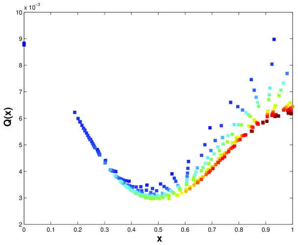
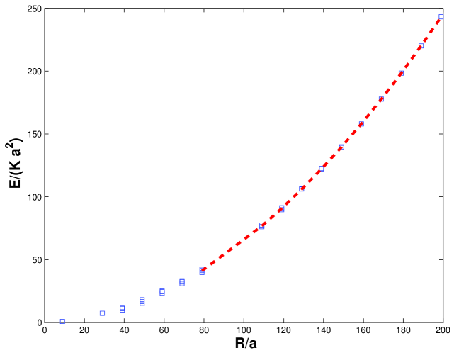
Figure 8: Plot of the scaling function Eq. 32 for $D=3$, $\lambda=\mu$, $m=5$ and $\Psi=\frac{\pi}{5}$ for sizes $R=10-200$ ($\lambda=\mu$).

Figure 9: fit Eq. 11 to the values $R\sim{l_{gb}}$.

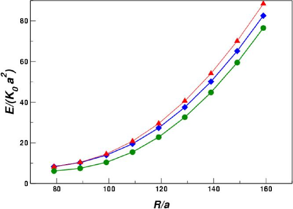
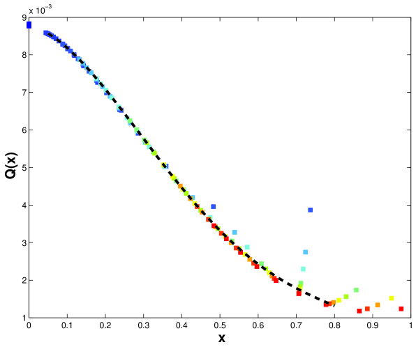
Figure 10: Comparison of different energies for $m=5$ and $D=5$ $\lambda=\mu$ for different values of $\Psi$.

Figure 11: Plot of the scaling function Eq. 32 for $D=7$, $\lambda=\mu$, $m=5$ and $\Psi=\frac{\pi}{5}$ for sizes $R=10-100$ ($\lambda=\mu$).

The ${\cal Q}$ function for $D$ values significantly different than $D_{crit}=\frac{5}{3}\pi$ are plotted in fig. 9 ($D=3$) and fig. 9 ($D=7$).

For $D<D_{crit}$ the scaling function has a minima as a function of $x$ in reasonable agreement with the value predicted by Eq. 34. As it is very apparent from fig. 9 the energy grows quadratically (compare with fig. 9) with the system size, even in the presence of the grain boundaries. The fit gives

$$\frac{E}{K_{0}R^{2}}=0.0055(4)\ .$$ (38)

This result should be compared with the theoretical estimate Eq. 53 for $\Pi=0$, $D=3$, $m=5$

$$\frac{E}{K_{0}R^{2}}=0.0039\ .$$ (39)

Although the result is not too different, the quantitative agreement is not very good. This may be attributed to assuming linear elasticity, which as already seen is not very accurate if disclinations are involved.

The energy for $D=7$ does not exhibit a minima because that should appear for values of $x>1$. The total energy for $D=7$ is significantly larger than for $D=5$, as it becomes apparent from the relative scale of the y-axis of the plot. The theoretical estimate Eq. 53 for $\Pi=0$, $D=7$, $m=5$ is

$$\frac{E}{K_{0}R^{2}}=0.0011\ .$$ (40)

The result in fig. 11 approaches this limit, although the statistics are not as good as in for $D=3$.

5.4 Dependence on the orientation of the grain $\Psi$

The dependence on the angle $\Psi$ is plotted in fig. 11 for angles $\Psi=0,\frac{\pi}{10},\frac{\pi}{5}$. Typical final relaxed configurations are shown in fig. 13 ($\Psi=\pi/5$) and fig. 13 ($\Psi=0$). The final relaxed configurations for $\Psi=\frac{\pi}{5}$ are very regular while the dislocations for the angle $\Phi=0$ display a rather jagged pattern. Provided that the total Burgers vector is zero, the only difference in the energies arises from the grain boundary terms. Therefore, the energy difference in the results fig. 11 should be attributed to the constraints induced by the lattice to the Burgers vector.This point might be substantiated numerically with a more comprehensive calculation, but this has not been done, partly because the angle $\Psi$ is not well defined for values of $m$ different than 5. The previous considerations reflect that the optimal angle for $m=5$ grain boundaries is given by $\Psi=\pi/5$.

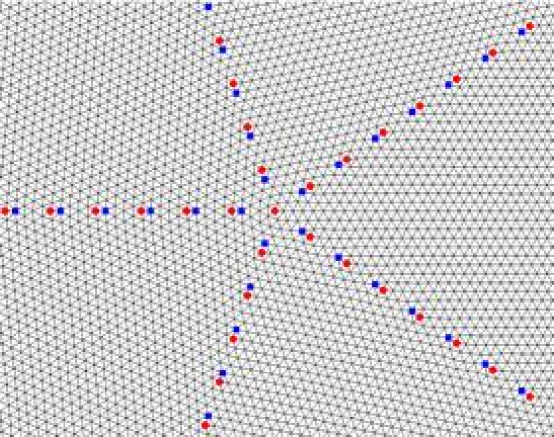
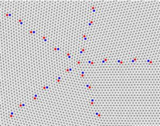
Figure 12: Final configurations for $m=5$, $D=5$ and $\Psi=\frac{\pi}{5}$ and $\lambda=\mu$. Results correspond to $R=90$.

Figure 13: Final configurations for $m=5$, $D=5$ and $\Psi=0$ and $\lambda=\mu$. Results correspond to $R=90$.

5.5 Dependence on the number of arms $m$

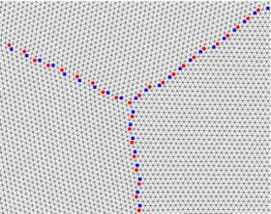
Figure 14: Relaxed configurations for $m=3$, $D=3$ and $\lambda=\mu$. Results correspond to $R=90$.

Figure 15: Relaxed configurations for $m=4$, $D=4$ and $\lambda=\mu$. Results correspond to $R=90$.

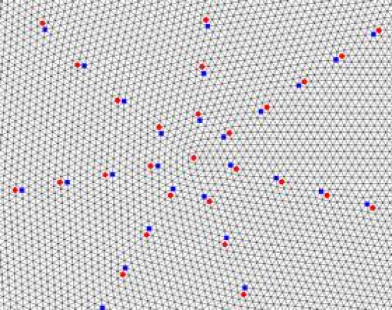
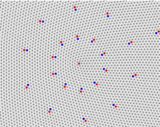
Figure 16: Relaxed configurations for $m=7$, $D=7$ and $\lambda=\mu$. Results correspond to $R=90$.

Figure 17: Relaxed configurations for $m=10$, $D=11$ and $\lambda=\mu$. Results correspond to $R=90$.

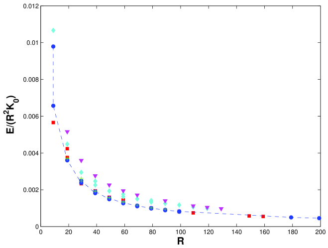
Figure 18: Plot of the energies for $l_{gb}\sim R$ as function of $R$ for $\lambda=\mu$. $m=3$ (square) $m=4$ (cross) $m=5$ (circle) $m=7$ diamond and $m=10$ (triangle down).

The analysis for different value of $m$ will be restricted to the optimal spacing values Eq. 9 and to the more relevant case $x\sim 1$ ($l_{gb}\sim R$). Some representative relaxed configurations are shown in fig. 15-17. Similarly as it was found in the investigation of the dependence on $\Psi$ subsect. 5.4 the constraint that dislocations can only be oriented along directions defined by the triangular lattice is the origin of additional frustration, leading to jagged arrangements which follow the ideal orientations only approximately.

The results corresponding to the energy are shown in fig. 18. For finite radius, the smaller values for $m$ are clearly favored. As $R$ becomes large the values for the energy become degenerate (within the numerical accuracy) in $m$ for $m$ within the range $m=2-5$. An evaluation of the $H$ function in Eq. 12 points out that the $m=2$ result should have the lowest energy. However, the difference in energy for arms $m=2-6$ are small compared with the core energy contribution, and at this precision, contributions from second order elasticity theory which have not been included may become important.

For larger $m$ the results show a larger energy, which is in qualitative agreement with the logarithmic dependence given by Eq. 13. Numerical results for large $m$ become increasingly difficult because it is difficult to direct the dislocations along the correct directions and also, because of the small number of dislocations per arm involved. A study including larger volumes than the ones performed here is necessary for more rigorous results. Finite size effects have been predicted to be negligible quadratically as a function of $m$ (see Eq. 12). The convergence is roughly consistent with that dependence.

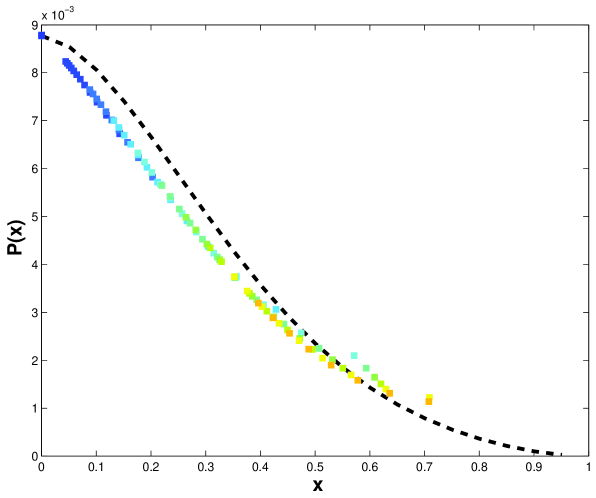
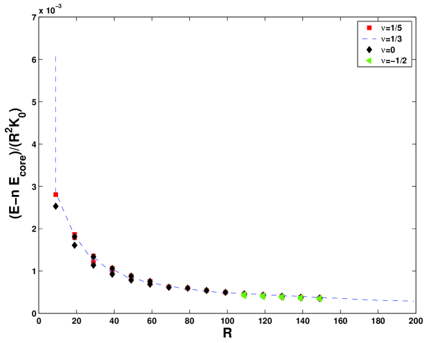
Figure 19: Plot of the scaling function Eq. 32 for $D=7$, $\lambda=\mu$, $m=7$ and $\Psi=\frac{\pi}{7}$ for sizes $R=10-200$. The dashed line is the universal function for a plus disclination.

Figure 20: Plot of the energy with the core energy contribution subtracted for $l_{gb}\sim R$ as function of $R$ for $m=5$ and different values of the Poisson ratio $\nu$.

5.6 Scaling collapse for minus disclinations

Results for minus disclinations have not been computed with the same accuracy as for positive ones. Nevertheless, the same trends as for fivefold defects are observed, as shown in fig. 20. The data collapses well to the assumed form Eq. 32, and the overall energy in the intermediate region is smaller than for fivefold defects.

6 Universality of the Results

The main assumption in the scaling forms for the energy Eq. 32 is that the only dependence on the elastic constants arises from the Young modulus. This is also true for all sub-leading terms, except for the core energy coefficient $c$ as it is obvious from table 1. Therefore, we will present the results by subtracting out the core energy contribution, and the results should then become universal.

Energy values for $x\sim 1$ plotted this way are shown in fig. 20. Except for very small systems, the universality hypothesis holds very well. Although cannot be conveyed from the plot, the energies for different Poisson ratio collapse to the same universal result with an accuracy less than $0.1\%$. This proves that the assumed form for the energy dependence is indeed universal, independent of the microscopic details of the lattice.

This universality of the ${\cal Q}$ function is also remarkable since the present calculation goes beyond linear elasticity, not only through the quadratic term in displacements kept in the strain tensor Eq. 23, but also through the higher powers of the strain tensor implicitly neglected in going from the discrete energy Eq. 19 to the continuum result Eq. 1. Those non-linear elasticity terms have shown to be quite important when disclinations are involved, and yet, do not seem to disturb in any way the scaling form assumed for the ${\cal Q}$ function. It seems reasonable then to assume that the results presented are not only universal with respect the two elastic constants, but also with respect to higher order terms in the elastic energy.

7 The Spherical Cap

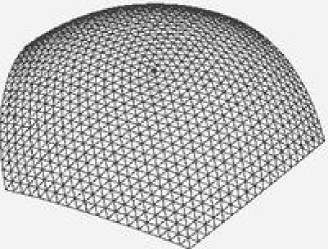
Figure 21: Crystal on an spherical cap. No additional dislocations are needed.

Although the results presented in this paper are interesting on their own, much of the motivation for carrying out such a project arises as an effort to provide efficient computational tools for investigating crystals on frozen geometries. We will therefore present a brief outline of some preliminary results for that problem. This will also provide a broader perspective of the versatility of the method.

Screening of disclination by grain boundaries is not the only mechanism available if disclinations are allowed to buckle out of the plane: Gaussian curvature without the need of additional grain boundaries is also a viable mechanism [4, 8].

An spherical cap of aperture angle $\gamma$ will have a Gaussian curvature $K=\frac{\gamma^{2}}{R^{2}}$. Therefore, for large $\gamma$ the Gaussian curvature will suffice to screen out the disclination and no additional dislocations will be needed. The limit of vanishingly small $\gamma$ has been discussed at length in this paper. Disclinations are screened out by grain boundaries going all the way to the boundary of the spherical cap. Therefore, for intermediate values of $\gamma$, structures of grain boundaries interpolating within these two cases should be observed [9].

The result of a minimization for large $\gamma$ is illustrated in fig. 21. It is found that, opposite to what happens for the flat case, additional dislocations actually increase the elastic energy of the system. One should notice that the triangles next to the boundaries are equilateral, which implies that the strains are very small (and so is the energy). A more detailed presentation of the results for crystals on spherical caps (positive curvature) including an investigation of the intermediate regime as well as a similar analysis for some minimal surfaces (negative curvature) will be presented elsewhere.

8 Conclusions

8.1 summary of the paper

The advantages of the computational method presented are:

1. Crystals with boundaries can be treated very efficiently.

2. There are no long range interactions. An entire sweep over the whole system may be performed with a time proportional to the total volume of the system.

3. The calculations may be extended to additional geometries with a negligible additional effort (only introducing the coordinates defining the geometry).

4. The convergence of the results (at zero temperature) is fast an stable.

5. The results are very universal, valid for a wide range of potentials. Microscopic details only enter via the elastic constants.

We provided a very detailed analysis for the problem of the dislocation cloud screening a disclination. It has been found that the system composed from a disclination charge $s$ and $m$-radial grain boundaries of dislocations separated a distance $D$ behaves as a single disclination with an effective charge

$$s_{eff}=s-m\frac{b}{D}\ .$$ (41)

If $s_{eff}=0$ then the total energy of the system grows linearly with the system size, similarly as for an infinitely long linear grain boundaries composed of dislocations only. The systems exhibits a remarkable universality with respect the elastic constants (up to core energy terms) and higher order elastic terms. The analytical expressions derived have been compared with the numerical results, and when disclinations are involved the discrepancy occasionally may be as large as $25\%$. Linear elasticity theory does not provide accurate quantitative estimates for the energetics of some problems involving disclinations.

8.2 Implications for Other problems

We will briefly discuss some of the implications the results found in this paper have for the problems presented in the introduction. It has been shown that for very small systems, grain boundaries with the smaller number of arms have the lowest energy. This is a general result in agreement with other continuum calculations [7] in the context of the sphere. The experimental results in Colloidosomes do show the same trends [5]. It would be very interesting to image larger Colloidosomes and analyze how the defect structures are changed, although that seems difficult in view of the equilibration times involved.

It has also been shown that if disclinations appear in a crystal phase, grain boundaries of dislocations should follow. Isolated disclinations are almost forbidden at zero temperature. At finite temperatures some properties of the grain will change, but for distances close enough to a disclination, the huge strains that dominate the energy will make additional dislocations inevitable. Strings ($m=2$ grains) or higher $m$ grains should surround the disclinations, even at finite temperature. Most of these grains will have a non-zero disclination charge (positive or negative). This qualitative picture seems in agreement with recent numerical [21] an experimental results [24, 23], where the correlation functions do show agreement with the KTHNY scenario (and therefore with the unbinding of disclinations) while the typical snapshots of configurations in equilibrium contain grain boundaries with non-zero disclination charge. Theories based on grain boundaries [26] ignore the possibility of having non-zero disclination charge from the very beginning. It has been shown in this paper that grain boundaries with non-zero disclination charge have energies comparable as grain boundaries of pure dislocations (with total disclination charge zero), provided the spacing within dislocations is fine tuned appropriately. A complete discussion of the temperature effects is obviously of great interest but it is beyond the scope of this paper.

8.3 Outlook

Some issues in this work need either further understanding or just higher precision data:

• Dynamic defect distribution: A global minimization for dislocation positions and orientations would directly provide the minimum energy configurations. This is a difficult task since it has been shown that the energy has many almost degenerate local minima.

• Non-integer spacings: Dislocations with non-integer spacings like $D=5\frac{\pi}{3}=5.23$, which imply that every third dislocation must be separated an additional lattice constant, have not been implemented. This may be of some importance in connection with Eq. 10.

• The degeneracy of the energy as a function of $m$ values should be further refined, since the accuracy of the results do not allow to discriminate for small values of $m$.

• The effects of an applied pressure has not been investigated numerically.

The computational method presented can be used to compute the energy of any distribution of defects in a two dimensional crystal. Results are in progress to investigate the effects of curvature and the interactions between disclinations.

We hope that the considerable detail presented in this paper will not obscure the main results obtained, but on the contrary, will provide convincing arguments for the utility of the present approach. The code used in this paper will be made publicly available. It may be also requested from the author.

ACKNOWLEDGMENTS

Many parts of this work arised as a result of many clarifying discussions with David Nelson, whom I cannot thank enough. I also acknowledge many interesting discussions with M. Bowick. I acknowledge S. Rotkin for explaining the interest of this problem in the context carbon nanotubes. This work has been supported by Iowa State University start-up funds.

Appendix A Energy of a disclination

The stresses of a single disclination at the origin may be computed from the Airy function of a disclination [4]

$$\chi=\frac{Gs}{2}(AR^{2}+r^{2}\log(r))\ ,$$ (42)

where $s=\frac{\pi}{3}q_{i}$,$G=\frac{K_{0}}{4\pi}$ and $A$ is an undetermined constant.

The stresses for a disclination are given by

$$\sigma_{yx}^{D} = -Gs\left[\frac{xy}{r^{2}}\right]$$

$$\sigma_{yy}^{D} = Gs\left[\frac{1}{2}+A+\frac{x^{2}}{r^{2}}-\log(l_{gb}/r)\right]$$ (43)

$$\sigma_{xx}^{D} = Gs\left[\frac{1}{2}+A+\frac{y^{2}}{r^{2}}-\log(l_{gb}/r)\right]\ ,$$

The stress along the radial direction is

$$\sigma_{rr}=\frac{K_{0}}{4\pi}(A+\frac{1}{2}+\log(r))$$ (44)

therefore, writing $A=-1/2+\frac{4\pi\Pi}{K_{0}}-\log(R)$, the stress at the boundary $R$ is $\sigma_{rr}=\Pi$, and $\Pi$ is interpreted as the two dimensional pressure the material.

Plugging Eq. A into Eq. 1, the energy becomes

$$F=\frac{s^{2}}{32\pi}K_{0}R^{2}+\frac{\pi\Pi^{2}}{8\cal{B}}R^{2},$$ (45)

where ${\cal B}=\mu+\lambda$ is the two dimensional bulk modulus. The result that the stress tensor Eq. A has an energy given by the expression Eq. 45 will be used quite frequently.

Appendix B Analytical proof of the optimal dislocation spacing

We will first compute the stresses generated by a finite grain boundary of length $l_{gb}$, with dislocations within the grain separated by distance $D$.

The stresses of a dislocation of Burgers vector $b$ located at the $y$ axis at point $(0,z)$ are given by

$$\sigma_{xy} = Gbx\frac{x^{2}-(y-z)^{2}}{(x^{2}+(y-z)^{2})^{2}}$$

$$\sigma_{yy} = -Gb(y-z)\frac{x^{2}-(y-z)^{2}}{(x^{2}+(y-z)^{2})^{2}}$$ (46)

$$\sigma_{xx} = Gb(y-z)\frac{3x^{2}+(y-z)^{2}}{(x^{2}+(y-z)^{2})^{2}}\ ,$$

where $G=\frac{K_{0}}{4\pi}$, where $K_{0}$ is the Young modulus. The total stresses will be computed from the methods used in dislocation pile-ups [41]. One obtains

$$\sigma_{xy} = \frac{Gb}{D}\int^{0}_{-l_{gb}}dzx\frac{x^{2}-(y-z)^{2}}{(x^{2}+(y-z)^{2})^{2}}$$ (47)

$$= -\frac{Db}{H}\left[\frac{yx}{y^{2}+x^{2}}-\frac{(y+l_{gb})x}{x^{2}+(y+l_{gb})^{2}}\right]$$

A similar calculation yields

$$\sigma_{yy} = -\frac{Gb}{D}\left[-\frac{x^{2}}{y^{2}+x^{2}}+\frac{x^{2}}{x^{2}+(y+l_{gb})^{2}}+\frac{1}{2}\log(\frac{x^{2}+(y+l_{gb})^{2}}{x^{2}+y^{2}})\right]$$ (48)

$$\sigma_{xx} = -\frac{Gb}{D}\left[\frac{x^{2}}{y^{2}+x^{2}}-\frac{x^{2}}{x^{2}+(y+l_{gb})^{2}}+\frac{1}{2}\log(\frac{x^{2}+(y+l_{gb})^{2}}{x^{2}+y^{2}})\right].$$

If the grain is now rotated and angle $\theta$ the stresses at distances $r<<l_{gb}$ will be (where $r=\sqrt{(}x^{2}+y^{2}$):

$$\sigma_{yx} = -\frac{Gb}{D}\left[\sin\theta\cos\theta+\frac{xy}{r^{2}}\right]$$

$$\sigma_{yy} = -\frac{Gb}{D}\left[-\frac{x^{2}\cos^{2}\theta}{r^{2}}+\frac{y^{2}\sin^{2}\theta}{r^{2}}+\log(l_{gb}/r)\right]$$ (49)

$$\sigma_{xx} = -\frac{Gb}{D}\left[\frac{x^{2}\cos^{2}\theta}{r^{2}}-\frac{y^{2}\sin^{2}\theta}{r^{2}}+\log(l_{gb}/r)\right]$$

Adding together $m$ arms separated an angle $\frac{2\pi}{m}$, one obtains

$$\sigma_{yx}^{G} = -m\frac{Gb}{D}\left[\frac{xy}{r^{2}}\right]$$

$$\sigma_{yy}^{G} = -m\frac{Gb}{D}\left[\frac{-x^{2}+y^{2}}{2r^{2}}+\log(l_{gb}/r)\right]$$ (50)

$$\sigma_{xx}^{G} = -m\frac{Gb}{D}\left[\frac{x^{2}-y^{2}}{2r^{2}}+\log(l_{gb}/r)\right]\ ,$$

where the identity $\sum_{l=1}^{m}\cos^{2}(\frac{2\pi l}{m})=\sum_{l=1}^{m}\sin^{2}(\frac{2\pi l}{m})=m/2$ has been used.

The stresses for a disclination have already been computed A with result

$$\sigma_{yx}^{D} = -Gs\left[\frac{xy}{r^{2}}\right]$$

$$\sigma_{yy}^{D} = Gs\left[\frac{1}{2}+A+\frac{x^{2}}{r^{2}}-\log(l_{gb}/r)\right]$$ (51)

$$\sigma_{xx}^{D} = Gs\left[\frac{1}{2}+A+\frac{y^{2}}{r^{2}}-\log(l_{gb}/r)\right]\ .$$

The total stresses are

$$\sigma_{yx}^{D} = -G(s-\frac{b}{D}m)\left[\frac{xy}{r^{2}}\right]$$

$$\sigma_{yy}^{D} = G(s-\frac{b}{D}m)\left[\frac{x^{2}}{r^{2}}-\log(l_{gb}/r)\right]+\Pi$$ (52)

$$\sigma_{xx}^{D} = G(s-\frac{b}{D}m)\left[\frac{y^{2}}{r^{2}}-\log(l_{gb}/r)\right]+\Pi\ ,$$

where the external pressure $\Pi$ is given by $\Pi=((A-1/2)s+\frac{b}{2H}m)G$. Using Eq. 45 for the modified disclination charge $s_{eff}=s-\frac{b}{D}m$, one finds

$$F=\frac{s_{eff}^{2}}{32\pi}K_{0}R^{2}+\frac{\pi\Pi^{2}}{8\pi{\cal B}}R^{2},$$ (53)

Therefore, perfect screening implies $s_{eff}=0$,

$$s=\frac{b}{D}m$$ (54)

and there is no external pressure $\Pi=0$, the system of disclination plus grain boundary does diverge quadratically with the system size. It can also be proved that within the same approach, the term linear in system size vanishes also. It should be emphasized that Eq. 54 is a linear order result. One should expect that if all orders were included, some modifications should occur, among them formula Eq. 54 should become Eq. 10

Appendix C Energy of a Grain boundary of dislocations

The energy of a linear grain boundary of $n$ dislocations with Burgers vector perpendicular to the grain is a well known result [40]. Here we just outline the aspects important for this paper. The total energy is given by

$$E=\frac{K_{0}a^{2}}{8\pi}n\int d^{2}{\bf r}\sigma_{xy}\ ,$$ (55)

where $\sigma_{xy}$ is the stress tensor of the dislocations in the $xy$ direction. The final result of the energy is

$$E=\frac{K_{0}a^{2}}{4\pi D}H(\frac{2\pi a}{D})R\ ,$$ (56)

where $a$ is the lattice constant and

$$H(x)=-\log(1-e^{-x})+\frac{x}{e^{x}-1}\ ,$$ (57)

for small $x$, (dislocations separated a distance $D>>a$), the usual formula $H(x)=-\log(x)+1$ follows. If $x$ is not small enough, the formula Eq 57 must be used.

Appendix D Relations of base vectors

If ${\bf e}_{1}$ and ${\bf e}_{2}$ are the triangular defining the triangular lattice the following relations follow.

$$\sum_{b}e^{i}_{ab}e^{j}_{ab}=3\delta^{ij}\ ,$$ (58)

where the sum is over all nearest neighbors $b$. It also follows

$$\sum_{b}e^{i}_{ab}e^{j}_{ab}e^{k}_{ab}e^{l}_{ab}=\frac{6}{8}(\delta^{ij}\delta^{kl}+\delta^{li}\delta^{kj}+\delta^{ki}\delta^{lj})$$ (59)

and

$$\sum_{b}e^{i}_{ab}e^{j}_{ab}e^{k}_{ab+1}e^{l}_{ab+1}=\frac{6}{8}(\delta^{ij}\delta^{kl}+R^{li}R^{kj}+R^{lj}R^{ki})\ ,$$ (60)

where $R^{ij}=\cos(\pi/3)\delta^{ij}+\sin(\pi/3)\epsilon^{ij}$. Similarly,

$$\sum_{b}e^{i}_{ab}e^{j}_{ab+1}e^{k}_{ab}e^{l}_{ab+1}=\frac{6}{8}(R^{ji}R^{lk}+R^{li}R^{jk}+\delta^{ki}\delta^{lj})\ ,$$ (61)

and

$$\sum_{b}e^{i}_{ab}e^{j}_{ab}e^{k}_{ab}e^{l}_{ab+1}=\frac{6}{8}(\delta^{ji}R^{lk}+R^{li}\delta^{jk}+\delta^{ik}R^{lj})\ .$$ (62)

References

- [1] D. R. Nelson. ”Defects and Geometry in Condensed Matter Physics”. Cambridge University Press, Boston, (2001).
- [2] P.P. Ewald. Ann. Phys. (Leipzig), 54:519, (1917).
- [3] K.J. Strandburg(editor). Bond Orientational Order in Condensed Matter. Springer-Verlag, (1992).
- [4] H. S. Seung and D. R. Nelson. ”defects in flexible membranes with crystalline order”. Phys. Rev. A, 38:1005, 1988.
- [5] A. Bausch et al. Science, 299:1716, (2003).
- [6] M. Spivak. ”Comprehensive Introduction to Diffferential Geometry”. Publish or Perish, Boston, (1979).
- [7] M. Bowick, D. R. Nelson, and A. Travesset. Phys. Rev. B, 62:8738, (2000).
- [8] M. Bowick and A. Travesset. J. Phys. A: Math. Gen., 34:1535–1548, (2001).
- [9] M. Bowick, A. Cacciuto, D. Nelson, and A. Travesset. Phys. Rev. Let., 89:185502, (2002).
- [10] M.J. W. Dodgson A. Perez-Garrido and M. A. Moore. Phys. Rev. B, 56:3640, (1997).
- [11] A. Toomre. private communication.
- [12] A. Perez-Garrido and M. A. Moore. Phys. Rev. B, 60:15628, (1999).
- [13] R Mosseri J P Gaspard and J F Sadoc. Taylor and Francis, London, (1982).
- [14] M. Rubinstein and D. R. Nelson. Phys. Rev. B, 28:6377, (1983).
- [15] M. Kleman and P. Donnadieu. Phylos. Mag., 52:121, (1985).
- [16] J. Sadoc and J. Charvolin. Acta Crystallogr. Sect. A, A45:10, (1989).
- [17] J. Kosterlitz and D. Thouless. J. Phys. C, 6:1181, (1973).
- [18] D.R. Nelson and B.I. Halperin. Phys. Rev. B, 19:2457, (1979).
- [19] A.P. Young. Phys. Rev. B, 19:1855, (1979).
- [20] K.J. Strandburg. Rev. Mod. Phys., 60:161, (1988).
- [21] F.L. Somer et al. Phys. Rev. Lett., 79:3431, (1998).
- [22] C. Reichhardt and C.J. Olson Reichhardt. Phys. Rev. Lett., 90:95504, (2003).
- [23] R.A. Quinn and J. Goree. Phys. Rev. E, 64:51404, (2001).
- [24] Tang et. al. Phys. Rev. Lett., 62:2401, (1989).
- [25] Markus et al. Phys. Rev. E, 60:5725, (1999).
- [26] S.T. Chui. Phys. Rev. B, 28:178, (1983).
- [27] Ch. Knobler and R. Desai. Annu. Phys. Chem., 43:207, (1992).
- [28] H. Mohwald V. Kaganer and P. Dutta. Rev. Mod. Phys., 71:779, (1999).
- [29] W. Lu et al. Phys. Rev. Lett., 89:146107, (2002).
- [30] M. Kelly D. Vaknin and B. Ocko. J. of Chem. Phys., 115:7697, (2001).
- [31] H. Diamant et al. Phys. Rev. E, 63:61602, (2001).
- [32] R. Pindak S.B. Dierker and R.B. Meyer. Phys. Rev. Lett., 56:1819, (1986).
- [33] L.N. Pfeiffer N.B. Zhitenev, R.C. Ashoori and K. W. West. Phys. Rev. Lett., 79:2308, (1997).
- [34] A.A. Koulakov and B. Shklovskii. Phys. Rev. B, 57:2352, (1998).
- [35] D.R. Nelson and L. Radzihovsky. Phys. Rev. A, 46:7474, (1992).
- [36] C. Carraro and D. R. Nelson. Phys. Rev. E, 48:19, (1993).
- [37] B. Halperin D. Fisher and R. Morf. Phys. Rev. B, 20:4692–4712, (1979).
- [38] S. Rotkin. private communication.
- [39] L. D. Landau and E. M. Lifshitz. Theory of Elasticity, volume 7 of Course of Theoretical Physics. Pergamon Press, Oxford, UK, 1986.
- [40] W.T. Read and W. Shockley. Phys. Rev., 78:275, (1950).
- [41] J. P. Hirth and J. Lothe. Theory of Dislocations. Wiley, NewYork, 1991.