Coexistence of antiferromagnetism and superconductivity in the Anderson lattice

Abstract

We study the interplay between antiferromagnetism and superconductivity in a generalized infinite-$U$ Anderson lattice, where both superconductivity and antiferromagnetic order are introduced phenomenologically in mean field theory. In a certain regime, a quantum phase transition is found which is characterized by an abrupt expulsion of magnetic order by $d$-wave superconductivity, as externally applied pressure increases. This transition takes place when the $d$-wave superconducting critical temperature, $T_{c}$, intercepts the magnetic critical temperature, $T_{m}$, under increasing pressure. Calculations of the quasiparticle bands and density of states in the ordered phases are presented. We calculate the optical conductivity $\sigma(\omega)$ in the clean limit. It is shown that when the temperature drops below $T_{m}$ a double peak structure develops in $\sigma(\omega)$.

1 Introduction

It is a common feature of several strongly correlated electronic systems that the low temperature ordered phases compete with each other. In particular, competition between antiferromagnetic and superconducting orders is an important characteristic of heavy-fermion systems[1], which is also shared by high-$T_{c}$ materials [2] and low-dimensional systems [3]. The closeness of the superconducting phase to the antiferromagnetic phase in heavy fermion compounds has lead to the conjecture that the attractive interaction leading to superconductivity is actually mediated by a magnetic excitation [1], instead of the traditional phonon mechanism. Also, the interplay between antiferromagnetism and superconductivity has been proposed to be described by a $SO(5)$ symmetry breaking [4]. The complexity of these systems arises from the interplay between Kondo screening of the local moments, the antiferromagnetic (RKKY) interaction between the local moments and superconducting correlations between the heavy quasiparticles.

Heavy fermion systems that exhibit both superconductivity and antiferromagnetism exhibit ratios between the Néel temperature $T_{N}$ and the superconducting critical temperature $T_{c}$ that can vary substantially (of the order of $T_{N}/T_{c}\sim 1-100$), with coexistence of both types of order below $T_{c}$. The coexistence of both types of order can be tuned by external parameters such as externally applied pressure or chemical pressure (involving changes in the stoichiometry).[1, 5] Examples of heavy-fermion materials which exhibit antiferromagnetic and superconducting order at low temperature are $URu_{2}Si_{2}$ and $U_{0.97}Th_{0.03}Be_{13}$. It has recently been found that $UPd_{2}Al_{3}$ ($T_{N}=14.3$ K and $T_{c}=2$ K) and $UNi_{2}Al_{3}$ ($T_{N}=4.5$ K and $T_{c}=1.2$ K) show coexistence of superconductivity and local moment antiferromagnetism. [1, 6, 7, 8, 9] However, in the $Ce$-based heavy-fermions magnetism tipically competes with superconductivity. In the prototype heavy-fermion system Ce_xCu₂Si₂ both coexistence and competition between $d-$wave superconductivity and magnetic order has been clearly observed in a small range of $x$ values around $x\simeq 0.99$ pressure.[5] This system exhibits a magnetic “A phase” at low temperature whose detailed nature is not yet known. Increasing pressure reduces the critical temperature $T_{A}$ of the A phase. Recent studies[5, 10, 11, 12] of $\rm CeCu_{2}Si_{2}$ samples near stoichiometric composition have shown that a $d$-wave superconducting phase expels the magnetic “A phase” when $T_{A}$ approaches $T_{c}$ under increasing pressure.

In general terms, the local moments due to the $f$-electrons are progressively quenched as the temperature lowers. In dilute systems the picture is well understood as due to the Kondo screening by the conduction electrons. In dense systems however the picture is more involved. At low temperatures the local moments are not completely quenched. In $U$-based materials such as $URu_{2}Si_{2}$, $UPt_{3}$ or $UPd_{3}$, for instance, the remaining moments are quite small of the order of $0.01-0.03\mu_{B}$ but for other systems such as $UPd_{2}Al_{3}$ the local moment is quite large of the order of $0.85\mu_{B}$. The low temperature magnetic behaviour of $Ce$-based compounds such as $CeCu_{2}Si_{2}$ and $CeCu_{6-x}Au_{x}$ has been interpreted as due to the vicinity to a quantum critical point [13] where the Néel temperature tends to zero. Two pictures arise however [14]: in the first one the Kondo temperature is high (the moments are quenched at a finite temperature) and when the system approaches the quantum critical point there are no free moments (assuming that quenching is complete). Then the system has to order due to a Fermi surface instability of the spin density wave type. Another possible situation is one in which the moments are not completely quenched down to $T=0$ and are free to orient themselves leading to magnetism. In the case of $CeCu_{6-x}Au_{x}$ evidence has been recently found that the second picture seems to hold [14] but a small but finite Kondo temperature has been quoted for this material (see the scond reference in [13]). On the other hand the high value of the Kondo temperature for the $CeCu_{2}Si_{2}$ compound [5] indicates possibly that the first scenario should hold. Furthermore, recent experiments [15] with $CeRh_{1-x}Ir_{x}In_{5}$ also reveal unusual coexistence of magnetism and superconductivity. It appears that in this system the $f$-electrons are more band-like than localized. On the other hand in $UPd_{2}Al_{3}$ it is the dual character of the $5f$ electrons that leads to the high value of the local moment in coexistence with the itinerant electrons and with the superconductivity [7].

On the theoretical side it is believed that the Anderson model and its extension to the lattice captures the basic physics of the heavy-fermions [16]. In this model the conduction electrons, $c$, (usually regarded as free) hybridize with local states, $f$, where the electrons are strongly interacting in such a way that the Coulomb repulsion, $U$, between two $f$-electrons is the largest energy scale in the problem. Frequently the limit $U\rightarrow\infty$ is taken implying that double occupancy is forbidden. The limit $U=\infty$ has been studied using the slave boson technique.[17, 18, 19] In particular, it has been shown that superconducting instabilities arise in the $p$ and $d$-wave channels because of the effective (RKKY) interaction between the $f-$electrons.[19, 20] Recently, the magnetic and superconducting instabilities of the normal phase were studied in the random phase approximation (RPA) [21] by taking into account slave boson fluctuations above the condensate. However, the competition/coexistence between both types of ordering was not considered.

In this work we consider the $U=\infty$ Anderson lattice model in the slave-boson approach. Because our aim is to study the interplay between magnetism and superconductivity, we explicitly introduce antiferromagnetic and superconducting couplings phenomenologically. The coupling constants are taken as independent even though they are related if the superconducting mechanism is mediated via the RKKY interaction. Using a mean-field approach we study directly the ordered phases and determine regimes of coexistence or competition between the two ordered phases depending on the parameters of the model.

In this work we will take the conduction electrons to be non-interacting but we should also mention that attempts to include interactions between the conduction electrons have been carried out [22, 23]. The inclusion of this more realistic interaction has been found to be required in some systems to attain a better understanding of the experimental results. We focus our attention on the coexistence of superconducting correlations and magnetic ordering in heavy fermions which, to our knowledge, has not yet been studied theoretically despite the considerable recent experimental effort devoted to this subject.

2 Model Hamiltonian and quasiparticle spectrum

The microscopic description of superconductivity and magnetic order in the Anderson lattice model is a still unsolved problem. In the folllowing we shall consider an effective Hamiltonian which originates from the $U=\infty$ Anderson model with two additional phenomenological terms: one where superconducting correlations are explicitly assumed between the local $f$-electrons (since it is believed that pairing occurs between heavy quasi-particles which, therefore, have essentially $f$ character) and another term where local spins are coupled antiferromagnetically. The infinite Coulomb repulsion between the $f$ electrons is described within Coleman’s slave-boson[18] technique with a condensation amplitude $\sqrt{z}$. The effective Hamiltonian is therefore:

$$H^{MF} = \sum_{k\sigma}(\epsilon_{k}-\mu)c_{k\sigma}^{\dagger}c_{k\sigma}+\sum_{k\sigma}(\epsilon_{f}-\mu)f_{k\sigma}^{\dagger}f_{k\sigma}$$ (1)

$$+ \sqrt{z}V\sum_{k\sigma}\left(f_{k\sigma}^{\dagger}c_{k\sigma}+c_{k\sigma}^{\dagger}f_{k\sigma}\right)$$

$$+ z\sum_{k}\left(\Delta_{f}\eta_{k}f_{k\uparrow}^{\dagger}f_{-k,\downarrow}^{\dagger}+\Delta_{f}^{*}\eta_{k}f_{-k,\downarrow}f_{k\uparrow}\right)$$

$$- 2m\sum_{k\sigma}\sigma\left(f_{k\sigma}^{\dagger}f_{k-Q,\sigma}+f_{k\sigma}^{\dagger}f_{k+Q,\sigma}\right)$$

$$+ (\epsilon_{f}-\epsilon_{0})(z-1)N_{s}+\frac{2N_{s}m^{2}}{J_{m}}-\frac{N_{s}|\Delta_{f}|^{2}}{J_{f}}$$

The $c$ and $f$ operators refer to conduction and localized electrons and obey the usual anticommutation relations. For simplicity, the hybridization potential $V$ is assumed to be momentum independent, $\epsilon_{0}$ and $\epsilon_{f}$ denote the bare and renormalized $f$-level energies, and $N_{s}$ denotes the number of lattice sites.

Although it is known that conduction electrons provide an effective RKKY interaction between $f$ electrons, we remark that the superconducting and magnetic order parameters in (1) cannot be simultaneously derived from a Hubbard-Stratonovich decoupling of a single RKKY term of the form ${\tilde{J}}_{ij}\vec{S}_{i}\cdot\vec{S}_{j}$, as discussed, for instance, in ref. [24] This is why we have phenomenologically introduced those terms.

In writing down the pairing term in (1) we have in mind that in the slave boson formulation a slave-boson operator $b_{i}$ is associated with every $f_{i}$ operator to prevent double occupancy. Condensation of the slave bosons is described by the replacement $b_{i}\rightarrow<b_{i}>=<b_{i}^{\dagger}>=\sqrt{z}$, hence the factor $z$ in the superconducting term of (1).[25, 26] The superconducting order parameter is given by $\Delta_{f}=\frac{zJ_{f}}{N_{s}}\sum_{k}\eta_{k}<f_{-k,\downarrow}f_{k\uparrow}>$, where $\eta_{k}$ denotes any of the possible pairing symmetries $\eta_{k}^{(s)}=\cos{k_{x}}+\cos{k_{y}}$, $\eta_{k}^{(p,i)}=\sqrt{2}\sin{k_{i}}$ and $\eta_{k}^{(d)}=\cos{k_{x}}-\cos{k_{y}}$ for $s$, $p$ and $d$ waves, respectively. Here we consider two dimensions for simplicitly of the calculations. We take a square lattice even though several heavy-fermions have a complicated lattice structure since we want to capture the main features.

The magnetic order parameter is given by the mean-field equation $m_{i}=J_{m}<f_{i\uparrow}^{\dagger}f_{i\uparrow}-f_{i\downarrow}^{\dagger}f_{i\downarrow}>$ and $m_{i}=2m\cos(\vec{r}_{i}\cdot\vec{Q})$ where $\vec{Q}=(\pi,\pi)$ is the antiferromagnetic ordering vector. We consider only commensurate antiferromagnetic correlations since it is particularly relevant to the systems referred.

In the calculations we assume a simple dispersion for the conduction electrons, of the form $\epsilon_{k}=-2t\sum_{i=x,y}\cos{k_{i}}$. For a given particle density the chemical potential must be computed from the condition $n_{c}+n_{f}=n$. The mean-field equations obtained from minimization of the free energy of Hamiltonian (1) are solved numerically. The solution gives the interplay between the boson condensation, the magnetization, and superconducting pairing as function of band-filling and of the various model parameters. Throughout this work we will consider only the case of $d$-wave pairing. The other two pairings give qualitatively similar results in most regimes as stressed before for the case of no magnetism and only superconducting order [25]. In different regimes different pairing symmetries become the most stable one but the overall behavior is similar. However we will get back to this point later. We will consider temperatures such that the slave bosons are condensed and therefore we quench the $f$-electron density fluctuations.

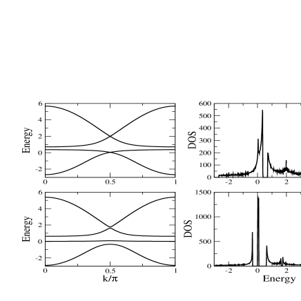
Figure 1: Quasiparticle bands and density of states for the magnetic coupling $J_{m}=0$ in the top panels and $J_{m}=0.9$ in the lower panels along the direction $k_{x}=k_{y}=k$. Model parameters are: $t=1$, $n=0.9$, $V=1.0$, and $\epsilon_{0}=-1.5$. The energies are measured with respect to the chemical potential.

2.1 Magnetic non-superconducting phase

We begin by discussing the magnetic but non-superconducting phase of the model. A detailed study of the superconducting non-magnetic phases has been presented elsewhere.[23, 25]

In order to diagonalize (1) for $J_{f}=0$ we introduce a quasi-particle operator which is a linear combination of the operators forming the basis $\left(c_{k\sigma}^{\dagger};c_{k+Q,\sigma}^{\dagger};f_{k\sigma}^{\dagger};f_{k+Q,\sigma}^{\dagger}\right)$. We write the Hamiltonian in this basis. The mean-field equations are obtained varying the effective Hamiltonian in the usual way. Minimization of the free energy of (1) with respect to $z$ gives:

$$\epsilon_{f}-\epsilon_{0}=-\frac{V}{2\sqrt{z}}\frac{1}{N_{s}}\sum_{k\sigma}\left(<f_{k\sigma}^{\dagger}c_{k\sigma}>+<c_{k\sigma}^{\dagger}f_{k\sigma}>\right)\,.$$ (2)

The condition $n_{f}+z=1$ reads:

$$z=1-\frac{1}{N_{s}}\sum_{k\sigma}<f_{k\sigma}^{\dagger}f_{k\sigma}>\,,$$ (3)

and the chemical potential is related to the total particle density as:

$$n=\frac{1}{N_{s}}\sum_{k\sigma}<c_{k\sigma}^{\dagger}c_{k\sigma}>+\frac{1}{N_{s}}\sum_{k\sigma}<f_{k\sigma}^{\dagger}f_{k\sigma}>\,.$$

The magnetization is given by:

$$m=\frac{J_{m}}{2N_{s}}\sum_{k\sigma}\sigma<f_{k\sigma}^{\dagger}f_{k-Q,\sigma}+f_{k\sigma}^{\dagger}f_{k+Q,\sigma}>\,.$$ (4)

For the sake of comparison, we show in Figure 1 the quasiparticle bands and the density of states for a situation where the magnetic order parameter is zero and nonzero, respectively. We see that in addition to the hybridization gap, there is an additional gap due to the magnetic order. The magnetic order with momentum $\vec{Q}$ reduces the size of the Brillouin zone to a half of that of a non-magnetic system.

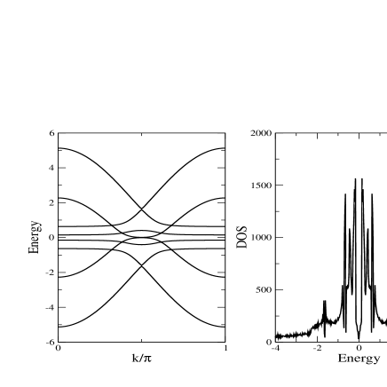
Figure 2: Quasiparticle bands and density of states for the couplings $J_{m}=0.9$, $J_{f}=-3$ for the Anderson model with magnetism and superconductivity. The other parameters are $n=0.9$, $V=0.6$, $\epsilon_{0}=-1.5$ and the hopping $t=V/0.66$.

2.2 Coexistence of antiferromagnetism and superconductivity

The Hamiltonian matrix $H_{k}$ can be written in the basis

$$\left(c_{k\uparrow},c_{k+Q,\uparrow},f_{k,\uparrow},f_{k+Q,\uparrow},c_{-k,\downarrow}^{\dagger},c_{-k-Q,\downarrow}^{\dagger},f_{-k,\downarrow}^{\dagger},f_{-k-Q,\downarrow}^{\dagger}\right)$$

as:

$$H_{k}=\left(\begin{array}[]{cc}A_{+}&D\\ D^{\dagger}&A_{-}\\ \end{array}\right)$$

where the matrices $A_{\pm}$ and $D$ are given by

$$A_{\pm}=\left(\begin{array}[]{cccc}\pm\epsilon_{k}&0&\pm\sqrt{z}V&0\\ 0&\pm\epsilon_{k+Q}&0&\pm\sqrt{z}V\\ \pm\sqrt{z}V&0&\pm\epsilon_{f}&-2m\\ 0&\pm\sqrt{z}V&-2m&\pm\epsilon_{f}\\ \end{array}\right)$$

and

$$D=\left(\begin{array}[]{cccc}0&0&0&0\\ 0&0&0&0\\ 0&0&z\Delta_{f}\eta_{k}&0\\ 0&0&0&z\Delta_{f}\eta_{k+Q}\\ \end{array}\right)$$

The energies are measured with respect to the chemical potential. The eigenvectors of the matrix $H_{k}$ are the Bogolubov operators expressed in the same basis.

Variation of the free energy with respect to $z$ shows that (2) must now be replaced by

$$\epsilon_{f}-\epsilon_{0} = -\frac{V}{2\sqrt{z}N_{s}}\sum_{\vec{k},\sigma}\left(<f_{\vec{k},\sigma}^{{\dagger}}c_{\vec{k},\sigma}>+<c_{\vec{k},\sigma}^{{\dagger}}f_{\vec{k},\sigma}>\right)$$ (5)

$$- \frac{2N_{s}}{zJ_{f}}\Delta_{f}^{2}$$

while the other mean-field equations remain unaltered.

In Figure 2 we show a typical quasiparticle band structure for the case where there is coexistence of magnetism and superconductivity. The quasiparticle bands are symmetric around the chemical potential due to the particle-hole structure of the Bogoliubov operators. Due to the superconducting order the spectrum is gapless.

3 Phase diagrams

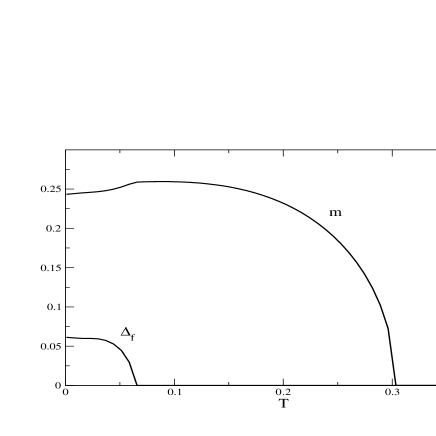
Figure 3: Magnetization and $d-$wave superconducting order parameters as functions of temperature for $n=1$, $t=1$, $\epsilon_{0}=-1.5$, $J_{f}=-3$, $J_{m}=0.9$, $V=0.66$.

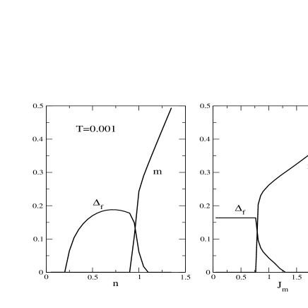
Figure 4: Magnetization and superconducting order parameters as functions of band-filling $n$ in the left panel and of $J_{m}$ in the right panel at a low temperature $T=0.001$. The other parameters are the same as in Figure 3.

The phase diagram of the model is quite rich due to the various correlations and order parameters considered. In this work we focus our attention on regimes where magnetism and superconductivity coexist or compete.

In Figure 3 we plot the magnetization and the $d$-wave superconducting order parameter as functions of temperature for a typical case. The critical temperature for the antiferromagnetic order parameter $m$, $T_{m}$, is larger than the critical temperature, $T_{c}$, for $d$-wave superconductivity. At low temperatures the two phases coexist. While $\Delta_{f}\rightarrow 0$ the magnetization $m$ is increasing and then $m$ decreases to zero at $T_{m}$ in the usual mean-field like manner.

The left panel of Figure 4 shows the order parameters $m$ and $\Delta_{f}$ as functions of band-filling at a fixed low temperature $T=0.001$. For low to intermediate band-fillings superconductivity exists. As the band-filling increases, the superconductivity is less favorable while the magnetic order parameter appears, as expected, since the magnetic order is more favored if the local electron density is higher. The value of $\Delta_{f}$ vanishes at low densities because the $f$-level occupancy also becomes small in that limit ($z\rightarrow 1$, $n_{f}\rightarrow 0$) and Cooper pairing occurs only between the $f$-electrons in the model considered. In the high density limit, $\Delta_{f}$ also tends to zero because the $f$-level occupancy is higher, approaching 1, and freezing of the charge fluctuations occurs due to the infinite on-site repulsion. Furthermore, a comparison with earlier results[25], where magnetic order was not considered, shows that magnetic order lowers the maximum value of the band-filling for which $\Delta_{f}\neq 0$, indicating that the two effects compete with each other. At smaller band-fillings incommensurate antiferromagnetic order also stabilizes. Indeed it extends to lower band-fillings as compared to the commensurate case. However the superconducting order expels the incommensurate case as well and including both types of ordering the phase diagram is qualitatively similar for commensurate or incommensurate order if superconductivity is also allowed.

The behavior of the order parameters against magnetic coupling, $J_{m}$, at low temperature, is shown in the right panel of Figure 4. Increasing $J_{m}$ leads to a crossover from a region where $m=0$ to a regime where $m$ grows with $J_{m}$ while $\Delta_{f}$ follows the opposite trend. Keeping $J_{m}$ fixed and decreasing $J_{f}$ leads to the opposite result where the superconductivity disappears in favor of magnetism.

In Figure 5 we plot the two critical temperatures as functions of the band-filling and of the hybridization. The behavior of the critical temperatures against density follows the same trend as in Figure 4: for low $n$ the superconducting temperature is higher while for higher densities $T_{m}>T_{c}$, indicating which phase is favored as one lowers the temperature from the disordered high temperature phase. Lowering $\epsilon_{0}$ or $V$ has the tendency to increase $f$-occupancy favoring magnetic order over superconducting order. At the point where the two temperatures cross the magnetic temperature falls abruptly to zero if the Cooper pairing symmetry is $d$-wave. This does not happen if the pairing symmetry is either extended $s$-wave or $p$-wave. In these cases there is no abrupt expulsion of the magnetization when the magnetic critical temperature becomes lower than the superconducting critical temperature and the phase where AF and SC coexist extends for smaller band-filling values and for larger values of the hybridization.

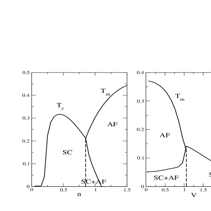
Figure 5: Critical temperatures $T_{c}$ and $T_{m}$ as functions of band-filling, $n$ and of $V$. The other parameters are the same as in Figure 3. The antiferromagnetic (AF), superconducting (SC) and coexisting phases (SC$+$AF) are shown

In the light of the experimental results, it is clearly interesting to compare qualitatively these results with the experimental phase diagrams, where either external pressure or chemical pressure are varied. Increasing pressure is expected to increase both hopping and hybridization amplitudes, while probably keeping $V/t$ and other parameters approximately constant, to a first approximation[27]. In Figure 6 we plot the mean field temperatures as functions of $V$ for fixed ratio $V/t$. As pressure increases the magnetic critical temperature decreases and $T_{c}$ increases. Once again at the point where the two temperatures cross the magnetic temperature falls abruptly to zero if the Cooper pairing symmetry is $d$-wave. This result, showing expulsion of a spin-density-wave by $d$-wave superconductivity but not in the case of the other symmetries, is very similar to that of a previous study[28] where the problem of local moment formation in a superconducting phase was addressed: increasing pressure causes expulsion of local moments by $d$-wave superconductivity. Therefore, such a phenomenon occurs either in a scenario of (unscreened or partially screened) ordered local moments or in a spin-density-wave scenario, where magnetic order appears as a Fermi surface instability.

The abrupt decrease of $m$ as $T_{c}$ crosses $T_{m}$ signals a quantum phase transition that can be tuned using the external pressure as a parameter: as pressure is reduced (at zero $T$) the groundstate of the system changes abruptly from nonmagnetic but superconducting to magnetic and superconducting at a critical value of $V_{c}$. The transition appears to be first order. We note that the same behavior is found for the compound $CeCu_{2}Si_{2}$ [29].

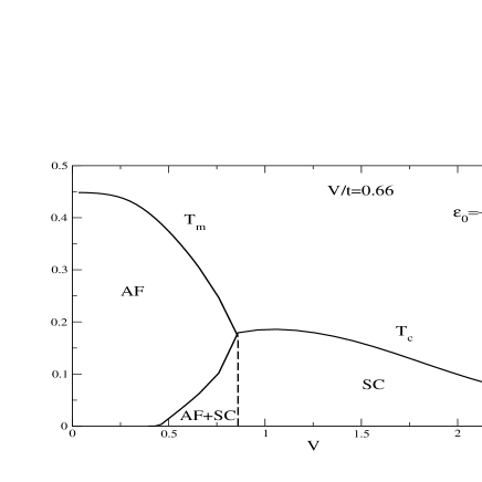
Figure 6: Critical temperatures $T_{c}$ and $T_{m}$ as functions of $V$, with fixed $V/t=0.66$ for $\epsilon_{0}=-1.5$. The other parameters are the same as in Figure 3. The antiferromagnetic (AF), superconducting (SC) and coexisting phases (SC$+$AF) are shown

Experimentally, most systems have quite large effective masses. Large mass enhancements are obtained when $z$ is small ($n_{f}\rightarrow 1$). This is indeed observed in regimes where the AF order parameter is large but in these regimes superconductivity is absent. In Figure 7 we show results for the quasiparticle bands and densities of states where a strong mass enhancement is seen for a large magnetization in opposition to a situation where the magnetization is zero. In the calculations above, we have not been able to find regimes where there is a very large (say larger than $200$) mass enhancement. In the model considered, the appearance of superconductivity is restricted to the mixed valent regime. In this situation we do not expect very large densities of states at the chemical potential. In a more realistic approach $U$ is large but finite and larger band-fillings are allowed ($0\leq n_{f}\leq 2$). We expect therefore that in this regime we might find large effective masses together with superconducting and magnetic order. The restriction to the mixed valent regime is a consequence of the slave boson approach [30]. In this method the chemical potential is always pinned to the lowest quasiparticle band, the density is always smaller than one, and the superconductivity only appears in the intermediate valence regime with moderate effective masses [31]. Nevertheless, our results reproduce qualitatively well the experimental phase diagrams and the competition between the $d$-wave superconducting and magnetic phases, such as that observed, for instance, in $CeCu_{2}Si_{2}$.

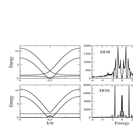
Figure 7: Top panels: Quasiparticle bands and density of states for the set of parameters $n=1$, $V=1.5$, $t=V/0.66$, $\epsilon_{0}=-1.5$, $J_{f}=-3$ and $J_{m}=0.9$. For this set of parameters the system is in a phase where $\Delta_{f}=0.108$, $m=0$ and $z=0.745$. Lower panels: Quasiparticle bands and density of states for the set of parameters $n=1.6$, $V=1.5$, $t=V/0.66$, $\epsilon_{0}=-1.5$, $J_{f}=-3$ and $J_{m}=0.9$. For this set of parameters the system is in a phase where $\Delta_{f}=0$, $m=0.412$ and $z=0.153$.

Model (1) is an effective Hamiltonian for the interacting $c$ and $f$ particles. Since the quasiparticles are heavy close to the top of the lowest band, as evidenced by the high values of the specific heat jump, we have modelled the superconducting interaction as taking place between the local $f$ electrons, as usual. One may wonder however the effect of adding a pairing term, with coupling constant $J_{c}$, between the $c$-electrons, since these are present at low energies close to the chemical potential. Considering a pairing term in the Hamiltonian in the standard way, with amplitude $\Delta_{c}$, we can solve the mean-field equations as before. The effect of this added term is shown in Figure 8. In general, the hybridization exchanges electrons between the $c$ and the $f$ levels. Due to the restriction on the level occupancy due to the infinite $U$ repulsion, for a fixed $V$ as the density increases the number of f-electrons decreases and the superconductivity is destroyed, as discussed above. However, if the $c$ electrons pair then the order parameter $\Delta_{c}$ increases. As a consequence in Figure 8 we see that as the density increases the ordering in the c-electrons increases. Actually, if we consider both types of pairing then the pairing in the f electrons extends to higher densities. So in that sense adding the pairing between the c electrons favors superconductivity at higher densities. However, we have found that the adddition of this type of pairing inhibits the magnetism in the f-electrons probably due to the greater stability in the pairing channel.

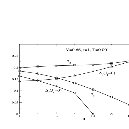
Figure 8: Superconducting order parameters $\Delta_{f}$ and $\Delta_{c}$ (see text) as functions of band-filling $n$ at a low temperature $T=0.001$ where we also include a $c$-electron pairing. The other parameters are the same as in Figure 3.

We remark however, that had we written a BCS pairing term only among the $c$-electrons in the Hamiltonian (1), the resulting phase diagram would be quite different: the superconducting temperature would be maximum at zero hybridization and rapidly decrease with increasing $V$. This is easily understood because increasing $V$ makes $c$-electrons heavier hence reducing their pairing amplitude. Clearly this is the opposite trend to that found experimentally in the phase diagrams as a function of pressure where, at low hybridizations, superconductivity is absent giving place to the magnetic order. Even if we do not include the possibility of magnetic order then it was shown before [25] that for small values of the hybridization the superconducting critical temperature is an increasing function of pressure. On the other hand, by having chosen a pairing interaction between $f$-electrons, we obtained increasing $T_{c}$ since the $f$-electrons become more mobile upon increasing $V$. Therefore it is justified to consider only a pairing term between the heavy f-electrons.

4 Optical and dynamic conductivity

The study of the particle-hole excitations of a system can be probed by studying the finite frequency conductivity. Studies of the Anderson lattice have been carried out previously [17, 32] in the disordered phases and experimental results for the heavy fermions have been reviewed in Ref [33]. In traditional superconductors the optical conductivity clearly shows a threshold at twice the gap energy[34, 35]. Since the d.c. conductivity of a perfect lattice is infinite, most studies are carried out taking into account scattering off impurities [36] considering moderate scattering up to the dirty limit [35, 36]. In this work we will study the optical conductivity in the clean limit and we shall study its behavior in the ordered phases as well.

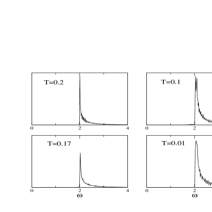
Figure 9: Optical conductivity (in arbitrary units) at several temperatures. $n=1$, $V=1.2$, $t=V/0.66$, $\epsilon_{0}=-1.5$, $J_{f}=-3$, $J_{m}=0.9$. For these parameters the system is superconducting at low temperatures and has no magnetization.

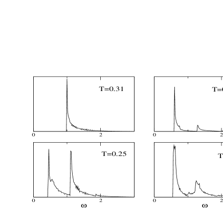
Figure 10: Optical conductivity (in arbitrary units) at several temperatures. $n=1$, $V=0.7$, $t=V/0.66$, $\epsilon_{0}=-1.5$, $J_{f}=-3$, $J_{m}=0.9$. For the parameters chosen magnetism and superconductivity coexist at low temperatures.

The real part of the dynamic conductivity is given by

$$\sigma_{\alpha\beta}(\vec{q},\omega)=\frac{1-e^{-\beta\omega}}{2\omega V}\int_{-\infty}^{\infty}dte^{i\omega t}<j_{\alpha}^{\dagger}(\vec{q},t)j_{\beta}(\vec{q},0)>$$ (6)

Writing the trace, inserting a decomposition of the identity in terms of the exact many-body energy states and integrating over time we obtain

$$\sigma_{\alpha\beta}(\vec{q},\omega) = \frac{1-e^{-\beta\omega}}{2\omega V}2\pi\sum_{n,m}\frac{e^{-\beta E_{n}}}{Z}\delta(\omega+E_{n}-E_{m})$$ (7)

$$<n|j_{\alpha}^{\dagger}(\vec{q})|m><m|j_{\beta}(\vec{q})|n>$$

Consider now $\alpha=\beta$ and $\vec{q}=0$. The $\alpha=x,y$ component of the current operator can be written as

$$j_{\alpha}=-it\sum_{\vec{k},\sigma}\left(\vec{\chi}_{\vec{k}}\right)_{\alpha}c_{\vec{k}\sigma}^{\dagger}c_{\vec{k}\sigma}$$ (8)

where $\vec{\chi}_{\vec{k}}=\sum_{\vec{\delta}}\vec{\delta}e^{-i\vec{k}\cdot\vec{\delta}}$ where $\sigma$ is the spin component. Writing the electronic operators in terms of the Bogolubov operators it is straightforward to calculate the matrix elements of the current operator.

We can also calculate the finite-momentum and finite-frequency conductivity $\sigma_{xx}(\vec{q},\omega)$. Starting from eq. (8) and taking similar steps to those followed for the calculation of the optical conductivity it is easy to calculate the dynamical conductivity.

In Figures 9 and 10 we show the optical conductivity in the clean limit for two typical cases. Figure 9 refers to a regime where there is superconductivity but no magnetization at low temperature. Figure 10 refers to a regime where there is coexistence of superconductivity and antiferromagnetism at low temperature.

The experimental study of the optical conductivity, over a large range of frequencies, of some heavy fermion systems has only recently become available. [37, 38] In reference [38] it was found that effective mass $m^{\ast}$ of the quasiparticles increased about 50 times when the temperature decreases below the Néel temperature. Furthermore, the authors found for $T<T_{N}$ that a two peak structure developed at finite frequencies. At temperatures higher than $T_{N}$ the $\sigma(\omega)$ presents a single peak, separated from the Drude weight by a finite gap (if disorder is included the Drude peak broadens to finite energies). When the temperature drops below $T_{N}$ a second peak, respecting to the magnetic gap, shows up in $\sigma(\omega)$ at lower, but finite, energies. The features reproduced by our calculation are in qualitative agreement with the data presented in Ref. [38]. Also they are in qualitative agreement with the results of [39]. Note however that our model is not appropriate to describe this material since one needs to take into account the dual nature of the f-electrons, which is not included in our model. This shows that the results obtained are qualitative general trends that are captured by our simplified model.

In order to preserve momentum the optical conductivity probes the transitions between different bands coupled by the current operator. If we allow that momentum is interchanged then the dynamic conductivity also probes excitations along the same band in addition to across bands. In Figs. 11, 12, 13 we present the dynamic conductivity for different points in the Brillouin zone in three typical situations. In Fig. 11 the set of parameters and temperature are such that the system is superconducting, in Fig. 12 the system is both superconducting and magnetic and in Fig. 13 the system is only magnetic. The gap structure evident in the optical conductivity ($\vec{q}=0$) is now absent because low energy excitations are in general allowed since there is coupling between states in the same band. In the superconducting case (but not magnetic) the dynamic conductivity extends to zero frequency but vanishes in this limit due to the energy dispersion of the $d$-wave symmetry. If there is coexistence of superconductivity and magnetism then the same structure appears with the double-peak feature, characteristic of the magnetic phase, enhanced, as observed in the optical conductivity. If the superconducting order parameter is zero then the dynamic conductivity is finite at zero energy.

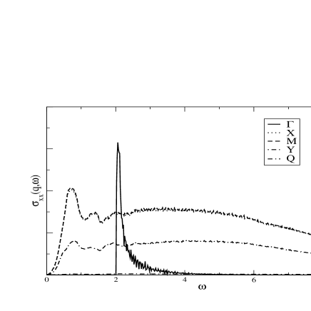
Figure 11: Finite-momentum and finite frequency conductivity at several points in the Brillouin zone for a set of parameters such that the system is superconducting ($\Gamma=(0,0),X=(\pi,0),M=(\pi,\pi),Y=(0,\pi),Q=(\pi/2,\pi/2)$). The temperature is $T=0.01$ and $V=1.2$. The results for the $\Gamma$ point, $\vec{q}=0$, are multiplied by 1000.

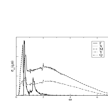
Figure 12: Finite-momentum and finite frequency conductivity at several points in the Brillouin zone for a set of parameters such that the system is superconducting and magnetic. The temperature is $T=0.01$ and $V=0.7$. The results for the $\Gamma$ point, $\vec{q}=0$, are multiplied by 1000.

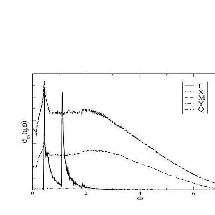
Figure 13: Finite-momentum and finite frequency conductivity at several points in the Brillouin zone for a set of parameters such that the system is magnetic. The temperature is $T=0.25$ and $V=0.7$. The results for the $\Gamma$ point, $\vec{q}=0$, are multiplied by 1000.

5 Summary

The interplay between magnetic correlations, the Kondo effect and superconducting correlations in heavy fermion systems is a difficult problem to solve. While previous studies on the $U=\infty$ Anderson lattice have identified the instabilities towards magnetic or superconducting order by taking into account the slave-boson fluctuations, the description of the ordered phases has not previously been carried out. In this work we have phenomenologically studied the interplay between the superconducting and antiferromagnetic ordered phases by studying their dependence on the model parameters. We have found that Cooper pairing symmetry plays an important role in determining the regimes of either coexistence or competition between superconductivity and antiferromagnetism: indeed, we have found that $d$-wave superconductivity coexists with antiferromagnetic order but the former expels the latter abruptly as the hybridization between the $f$-level and the conduction electrons increases. We also found that the $f$-level occupancy affects the two types of order in different ways: higher occupancy favors antiferromagnetism while a lower occupancy favors superconductivity. Hence, the quasiparticle mass enhancement relative to the bare electron was found not to exceed a few tens in the superconducting phase. The optical conductivity has also been computed, reflecting the band structure of the ordered phases.

References

References

- [1] N. D. Mathur, F. M. Grosche, S. R. Julian, I. R. Walker, D. Freye, R. Haselwimmer, and G. Lonzarich, Science 394, 39 (1998).
- [2] M. B. Maple, cond-mat/9802202.
- [3] C. Bourbonnais and D. Jèrome, Science 281, 1155 (1998).
- [4] S. C. Zhang, Science 275, 1089 (1997); E. Arrigoni, M. G. Zacher, T. Eckl and W. Hanke, cond-mat/0105125.
- [5] K. Ishida, Y. Kawasaki, K. Tabuchi, K. Kashima, Y. Kitaoka, K. Asayama, C. Geibel, and F. Steglich Phys. Rev. Lett 82, 5353 (1999).
- [6] R. Caspary, P. Hellmann, M. Keller, G. Sparn, C. Wassilew, R. Köhler, C. Geibel, C. Schank, F. Steglich, and N. Phillips, Phys. Rev. Lett. 71, 2146, (1993).
- [7] R. Feyerherm, A. Amato, F. N. Gygax, A. Schenck, C. Geibel, F. Steglich, N. Sato, and T. Komatsubara, Phys. Rev. Lett. 73, 1849 (1994).
- [8] N. Bernhoeft, N. Sato, B. Roessli, N. Aso, A. Hiess, G. H. Lander, Y. Endoh, and T. Komatsubara, Phys. Rev. Lett. 81, 4244 (1998);
- [9] N. Aso, B. Roessli, N. Bernhoeft, R. Calemczac, N.K. Sato, Y. Endoh, T. Komatsubara, A. Hien, G.H. Lander, H. Kadowaki, Phys. Rev. B 61, R11867 (2000).
- [10] P. Gegenwart, C. Langhammer, C. Geibel, R. Helfrich, M. Lang, G. Sparn, F. Steglich, R. Horn, L. Donnevert, A. Link and W. Assmus, Phys. Rev. Lett. 81, 1501 (1998)
- [11] G. Bruls, B. Wolf, D. Fisterbush, P. Thalmeier, I. Kouroudis, W. Sun, W. Assmus, B. Lüthi, M. Lang, K. Gloos, F. Steglich and R. Modler, Phys. Rev Lett. 72, 1754 (1994)
- [12] G. M. Luke, A. Keren, K. Kojima, L. P. Le, B. J. Sternlieb, W. D. Wu, and Y. J. Uemura, Phys. Rev Lett. 73, 1853 (1994)
- [13] F. Steglich, B. Buschinger, P. Gegenwart, M. Lohmann, R. Helfrich, C. Langhammer, P. Hellmann, L. Donnevert, S. Thomas, A. Link, C. Geibel, M. Lang, G. Sparn and W. Assmus, J. Phys. Cond. Matt. 8, 9909 (1996); H. von Löhneysen, J. Phys. Cond. Matt. 8, 9689 (1996).
- [14] A. Schröder, G. Aeppli, R. Coldea, M. Adams, O. Stockert, H. v. Löhneysen, E. Bucher, R. Ramazashvili and P. Coleman, Nature 407, 351 (2000).
- [15] P. G. Pagliuso, C. Petrovic, R. Movshovich, D. Hall, M. F. Hundley, J. L. Sarrao, J. D. Thompson and Z. Fisk, Phys. Rev. B 64, 100503 (2001).
- [16] D. M. Newns and N. Read, Adv. Phys. 36, 799 (1987).
- [17] A.J. Millis and P.A. Lee, Phys. Rev B 35, 3394 (1987).
- [18] P. Coleman, Phys. Rev B 29, 3035 (1984); Phys. Rev B 35, 5072 (1987).
- [19] A. Houghton, N. Read, and H. Won, Phys. Rev. B 37, 3782 (1988).
- [20] M. Lavagna, A. J. Millis and P. A. Lee, Phys. Rev. Lett. 58, 266 (1987).
- [21] N. M. R. Peres and M. A. N. Araújo, J. Phys. Cond. Matt. 14, 5575 (2002).
- [22] T. Brugger, T. Schreiner, G. Roth, P. Adelmann and G. Czjzek, Phys. Rev. Lett. 71, 2481 (1993); P. Fulde, V. Zevin and G. Zwicknagl, Z. Phys. B 92, 133 (1993); G. Khaliullin and P. Fulde, Phys. Rev. B 52, 9514 (1995). T. Schork and S. Blawid, Phys. Rev. B 56, 6559 (1997). W. Hofstetter, R. Bulla and D. Vollhardt, Phys. Rev. Lett. 84, 4417 (2000).
- [23] L. P. Oliveira and P. D. Sacramento, Phys. Rev. B 66, 014516 (2002).
- [24] M. U. Ubbens and P. A. Lee, Phys Rev. B 46, 8434 (1992).
- [25] M.A.N. Araújo, N.M.R. Peres, P.D. Sacramento, and V.R. Vieira, Phys. Rev. B 62, 9800 (2000).
- [26] A. E. Ruckenstein, P. J. Hirschfeld and J. Appel, Phys. Rev. B 36, 857 (1987).
- [27] B. H. Bernhard and C. Lacroix, Phys. Rev. B 60, 12149 (1999).
- [28] M. A. N. Araújo, N. M. R. Peres and P. D. Sacramento, Phys. Rev. B 65, 012503 (2001).
- [29] Y. Kitaoka, Y. Kawasaki, T. Mito, S. Kawasaki, G. -q. Zheng, K. Ishida, D. Aoki, Y. Haga, R. Settai, Y. Onuki, C. Geibel and F. Steglich, cond-mat/0201040.
- [30] L. H. C. M. Nunes, M. S. Figueira and E. V. L. de Mello, cond-mat/0301126.
- [31] U. Rauchschwalbe, W. Lieke, F. Steglich, C. Godart, L. C. Gupta and R. D. Parks, Phys. Rev. B 30, 444 (1984); S. K. Malik, A. M. Umarji, G. K. Shenoy, and M. E. Reeves, J. Magn. Magn. Mater. bf 54, 439 (1986).
- [32] M. J. Rozenberg, G. Kotliar and H. Kajueter, Phys. Rev. B 54, 8452 (1996).
- [33] L. Degiorgi, Rev. Mod. Phys. 71, 687 (1999).
- [34] N. E. Bickers, D. J. Scalapino, R. T. Collins and Z. Schlesinger, Phys. Rev. B 42, 67 (1990).
- [35] H. Chen, Phys. Rev. Lett. 71, 2304 (1993).
- [36] D. C. Mattis and J. Bardeen, Phys. Rev. 111, 412 (1958).
- [37] S.V. Dordevic, D. N. Basov, N. R. Dilley, E. D. Bauer, M. B. Maple, Phys. Rev. Lett. 86, 684 (2001).
- [38] M. Dressel, N. Kasper, K. Petukhov, B. Gorshunov, G. Grüner, M. Huth, and H. Adrian, Phys. Rev. Lett. 88, 186404 (2002); M. Dressel, N. Kasper, K. Petukhov, D. N. Peligrad, B. Gorshunov, M. Jourdan, M. Huth, and H. Adrian, Phys. Rev. B 66, 035110 (2002).
- [39] N. K. Sato, N. Aso, K. Miyake, R. Shiina, P. Thalmeier, G. Varelogiannis, C. Geibel, F. Steglich, P. Fulde and T. Komatsubara, Nature 410, 340 (2001).