Weakly nonlinear subcritical instability of visco-elastic Poiseuille flow

Abstract

It is well known that the Poiseuille flow of a visco-elastic polymer fluid between plates or through a tube is linearly stable in the zero Reynolds number limit, although the stability is weak for large Weissenberg numbers. In this paper we argue that recent experimental and theoretical work on the instability of visco-elastic fluids in Taylor-Couette cells and numerical work on channel flows suggest a scenario in which Poiseuille flow of visco-elastic polymer fluids exhibits a nonlinear “subcritical” instability due to normal stress effects, with a threshold which decreases for increasing Weissenberg number. This proposal is confirmed by an explicit weakly nonlinear stability analysis for Poiseuille flow of an UCM fluid. Our analysis yields explicit predictions for the critical amplitude of velocity perturbations beyond which the flow is nonlinearly unstable, and for the wavelength of the mode whose critical amplitude is smallest. The nonlinear instability sets in quite abruptly at Weissenberg numbers around 4 in the planar case and about 5.2 in the cylindrical case, so that for Weissenberg numbers somewhat larger than these values perturbations of the order of a few percent in the wall shear stress suffice to make the flow unstable. We have suggested elsewhere that this nonlinear instability could be an important intrinsic route to melt fracture and that preliminary experiments are both qualitatively and quantitatively in good agreement with these predictions.

I Introduction

I.1 General motivation

In this paper, we reconsider the classical topic of the stability of visco-elastic Poiseuille flow in the zero Reynolds number limit. From a weakly nonlinear expansion, we find that this flow is nonlinearly unstable for high enough flow rates.

The first linear stability analysis of the flow of a so-called Oldroyd-B fluid — one of the simplest continuum models for a visco-elastic polymeric fluid with nonzero normal stress differences, characterized by a single relaxation time $\lambda$ bird — was already performed almost thirty years ago denn2 . Since the subsequent careful linear stability analysis of Ho and Denn denn1 it is generally accepted that Poiseuille flow of an Oldroyd-B fluid is linearly stable, even though the stability is weak for large values of the Weissenberg number, the dimensionless quantity which measures the strength of polymer relaxation effects. The definition used in this paper for the case of cylindrical coordinates relevant for pipe flow is

$${\sf Wi}=\left.\frac{\tau_{rr}-\tau_{zz}}{\tau_{rz}}\right|_{\text{wall}},$$ (1)

where the term in the numerator is the normal stress difference of the flow. For the planar geometry the index $r$ has to be replaced by $y$, with the $y$-axis taken normal to the plates. The term in the denominator of (1) is the shear stress at the wall. For an Oldroyd-B or Upper Convected Maxwell (UCM) fluid, the unperturbed flow field $v^{\text{unp}}$ is simply parabolic, and we get

$${\sf Wi}=2\lambda\left.\frac{\partial v^{\text{unp}}_{z}}{\partial r}\right|_{\text{wall}}=4v_{\text{max}}\lambda/R.$$ (2)

Here $v_{\text{max}}$ is the maximum velocity of the unperturbed profile, $\lambda$ is the aforementioned relaxation time characterizing the Oldroyd-B or UCM fluid, and $R$ is the radius of the pipe. For the planar case, R has to be replaced by $d$, half the spacing between the plates.

It is well known that visco-elastic Poiseuille flow is linearly stable for well-established models like the UCM, Oldroyd-B denn1 and the Giesekus model keunings . However, there are good reasons to reconsider the nonlinear instability of this flow configuration. First of all, Atalik and Keunings keunings have recently presented strong numerical evidence tht visco-elastic Poiseuille flow is indeed nonlinearly unstable for the UCM, Oldroyd-B and Giesekus model: when they injected the laminar flow field with a perturbation of sufficiently large amplitude, instead of dying out (like one would expect for a strictly stable flow) the perturbation grew and saturated at a finite value, resulting in a finite amplitude oscillatory flow. Such behavior, in which the flow is always linearly stable but nonlinearly unstable, is also called a subcritical instability. A recent experiment yesilata also supports this nonlinear instability scenario. Secondly, as we will discuss in detail in section I.2 below, there are actually a lot of indirect indications from well-established results on visco-elastic Taylor-Couette flow that planar Couette or Poiseuille flow between plates or in a tube might have a subcritical instability. Last but not least is the following observation: if visco-elastic Poiseuille flow is unstable, the nonlinear spatially and temporally oscillatory flow pattern it will give rise to will inevitably result in distortions of the flow after exiting the pipe or slit. In other words, if visco-elastic Poiseuille flow is unstable for large enough ${\sf Wi}$, it automatically leads to an intrinsic route to “melt-fracture” type phenomena, a generic name for the fact that a polymer extrudate normally develops strong undulations or irregularities beyond some critical flow rate denn3 ; denn4 ; pahl . It is well-established that there are various mechanisms that can lead to such type of behavior (e.g., stick-slip behavior or exit instabilities leading to sharkskin type patterns denn3 ; denn4 ). Most of these can be (partially) suppressed by the proper choice of material or of the extruder shape and coating. Our main conclusion (in line with keunings ) that polymer Poiseuille flow is nonlinearly unstable for large enough ${\sf Wi}$ implies that melt fracture type behavior is an unavoidable consequence of a nonlinear instability in the extruder. In this paper, we focus on the subcritical instability of visco-elastic Poiseuille flow itself. Our arguments and experimental support for this scenario are summarized in two recent letters meulenbroek ; bonn1 , but the issue is complex and deserves further experimental and theoretical study. We will come back to it in the future.

As stated, the calculations that we report in this paper give the details of the explicit nonlinear amplitude expansion for the stability of visco-elastic Poiseuille flow in the case of fixed average pressure gradient (we consider periodic modulations of the pressure, so there are periodic pressure modulations but the average pressure drop remains unchanged). We show explicitly that for large values of ${\sf Wi}$ there is indeed subcritical behavior, in other words that the flow exhibits a weakly nonlinear instability. Moreover, the subcritical behavior sets in quite abruptly around a value ${\sf Wi}_{\text{c}}$ of order 5 for flow in a tube. This value is consistent with the value where melt fracture type behavior is normally reported to set in denn3 ; denn4 ; pahl , but somewhat larger than the critical value of 0.1 found numerically for for the related Oldroyd-B model with viscosity contrast $10^{-3}$ and a Reynolds number of 0.1 keunings . We will discuss the possible origins of these discrepancies at the end of this paper.

Since the nonlinear amplitude expansion that we will employ has been used mostly in other fields of physics, and since it involves some unusual subtleties, we present our results in some detail. For the benefit of the reader not interested in the derivation, we summarize our main results in section I.3 of this introduction. Before doing so, we first discuss the relation of this work with the Taylor-Couette problem.

I.2 A nonlinear instability scenario motivated by the visco-elastic Taylor-Couette problem

Just over a decade ago, Larson et al. larson investigated the stability of the flow of a visco-elastic polymer solution in a Taylor-Couette cell, a cell consisting of two concentric rotating cylinders. They found that in this system the flow does exhibit a well-defined linear instability for some value of the Deborah number ${\sf De}$, which is analogous to the Weissenberg number. Their calculations were done for the Oldroyd-B polymer model. In the same paper the predictions were confirmed experimentally by a series of measurements on a polymer solution which is well described by this model. This work was later extended by Joo and Shaqfeh shaqfeh0 ; shaqfeh1 , who considered the more general case of flow in a curved channel. In the limit of boundary driven flow this reduces to the Taylor-Couette case, while in the limit of static curved walls the flow is driven by a pressure gradient (so-called Dean flow). In all these cases, as well as in the experimentally relevant cone and plate geometry phantien1 ; phantien2 , the flow is linearly unstable at large enough flow velocities. The main conclusion from this line of research has therefore been that a linear instability occurs in visco-elastic fluids due to “hoop stresses” if the stream lines are curved shaqfeh2 ; pakdel . This is confirmed by the observation that the various stability calculations show that the instability threshold goes to infinity if the curvature of the walls goes to zero. For the Taylor-Couette system this is the limit in which the radius of the cylinders goes to infinity; for the Dean flow problem investigated by Joo and Shaqfeh shaqfeh0 ; shaqfeh1 this result is consistent with the weak stability of Poiseuille flow between two parallel planes.

In the last few years, Groisman and Steinberg steinberg1 ; steinberg2 have experimentally investigated the visco-elastic instability in the Taylor-Couette system in detail. They find very good agreement with the theory for the onset of the instability when the polymer flow velocity is increased; however, an important result of their careful study is that the bifurcation at the critical Weissenberg/Deborah number is subcritical or “backward” steinberg2 ; sureshkumar .

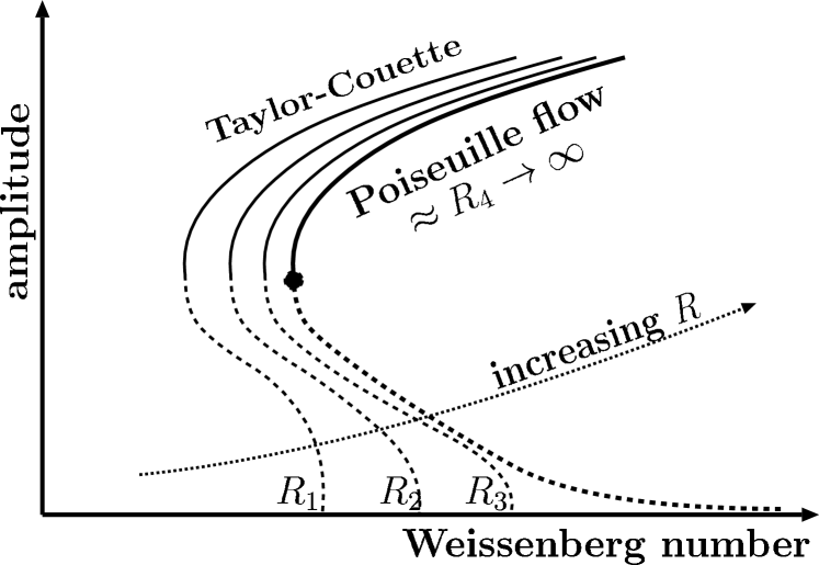
Figure 1: Qualitative sketch of the subcritical behavior of the visco-elastic instability in low Reynolds number polymer flow in a Taylor-Couette cell, and of our proposal that the bifurcation curve for the case of Poiseuille flow should be thought of as the limit in which the radius in the Taylor-Couette cell goes to infinity. See text.

Groisman and Steinberg steinberg2 have also presented intuitive arguments why the instability in visco-elastic Taylor-Couette flow at low Reynolds numbers is subcritical. In their arguments the fact that the flow is occurring between curved walls is playing essentially no role: the curvature of the walls is necessary to make the flow linearly unstable, but the nonlinear positive feedback mechanism that in their picture gives rise to the subcritical behavior does not rely on the curvature. This suggests the scenario sketched in Fig. 1: The stable nonlinear flow behavior, indicated in the figure by the full lines, is quite independent of the precise radius or curvature of the cylinders, assuming the “gap” (distance) between the cylinders to be constant. The points where the curves touch the horizontal axis correspond to the linear instability threshold. These points therefore are strongly dependent on the curvature of the cylinders: as indicated in the figure, the results of the theoretical analysis shaqfeh0 ; shaqfeh1 ; shaqfeh2 imply that they shift to the right as the radius $R$ of the inner cylinder increases, and that there is no linear instability in the limit $R\to\infty$.

The continuity found by Joo and Shaqfeh shaqfeh0 ; shaqfeh1 in going from the Taylor-Couette flow to the case of Poiseuille-like Dean flow between fixed curved planes, as well as the intuitive arguments of Groisman and Steinberg steinberg2 strongly suggest that the scenario for Poiseuille-flow through a channel will be very close to the one sketched in Fig. 1 for the limit $R_{4}\to\infty$: the unperturbed flow is linearly stable for any ${\sf Wi}$, but nonlinearly unstable as if there is a subcritical bifurcation at ${\sf Wi}=\infty$. Moreover, just like the rightmost curve for $R_{4}\to\infty$ approaches the horizontal axis rapidly for sufficiently large ${\sf Wi}$, implying that the threshold for the nonlinear instability is small at large ${\sf Wi}$, we expect that the threshold for the subcritical-like nonlinear instability of visco-elastic Poiseuille flow is small for sufficiently large ${\sf Wi}$. The work done in this paper, summarized in the next subsection, fully confirms this expectation.

It is of interest to note that the scenario we propose here for visco-elastic fluids in the zero Reynolds number limit has strong similarities for large Reynold number planar Poiseuille flow of Newtonian fluids: planar Poiseuille flow of ordinary fluids becomes linearly unstable at a Reynolds number of 5772, but in practice the flow becomes unstable at much lower Reynolds numbers of orszag ; huerre ; grossmann . Thus the transition is subcritical. The scenario that has emerged is that the nonlinear branch extends down to ${\sf Re}\approx 2500$ for two-dimensional perturbations and to ${\sf Re}\approx 1000$ for three-dimensional flows, and in fact already over thirty years ago pekeris ; hocking ; herbert2 ; herbert1 , an amplitude expansion for planar Poiseuille flow in the spirit of ours was instrumental in showing that the instability at ${\sf Re}=5772$ is subcritical. The scenario we propose for visco-elastic flow is even closer to the one that is found for the transition to turbulence in Poiseuille flow of Newtonian fluids in a pipe: although the flow is also linearly stable for any ${\sf Re}$, the flow is nonlinearly unstable for ${\sf Re}\gtrsim 1000$ with a threshold which decreases as ${\sf Re}^{-\gamma}$ for ${\sf Re}\to\infty$ chapman , very much like we suggest in Fig. 1 with the dashed line labeled $R_{4}\to\infty$. The transition to turbulence of Newtonian fluids therefore shows that whether or not there is a true linear instability is not very relevant in practice, and we believe that this is true for visco-elastic flows too.

Let us conclude this subsection with the following observation. As noted in the preceding paragraphs, it is generally accepted that when the stream lines are curved, visco-elastic flow becomes linearly unstable at sufficiently large flow rates. In accord with this visco-elastic Poiseuille flow is linearly stable since its stream lines are straight: infinitesimal perturbations must and do decay. However, following this same line of reasoning it is also very natural for visco-elastic Poiseuille flow or planar Couette to be nonlinearly unstable: in the presence of a finite perturbation, the stream lines are curved, and consequently we expect the flow to be unstable to any finite perturbation for sufficiently large flow rates. This is the essence of the subcritical instability scenario sketched above.

I.3 Summary of our main result for Poiseuille flow in the UCM model

In this paper we will consider the limit that the Reynolds number ${\sf Re}$

$${\sf Re}=\frac{Rv}{\eta/\rho},$$ (3)

is negligible. Here $R$ is a characteristic length scale ($d$ for the planar case, the radius $R$ for the case of a cylindrical tube), $v$ a characteristic velocity, $\rho$ the density and $\eta$ the viscosity of the fluid. As ${\sf Re}$ measures the strength of the inertial terms with respect to the viscous terms, in the limit ${\sf Re}\downarrow 0$ we can ignore the nonlinear convective terms in the momentum (Navier-Stokes) equation, and make a quasistationary approximation in which the temporal derivatives in the momentum equation are neglected.

As stated before, as the constitutive equation for the polymer fluid we take the so-called UCM (Upper Convected Maxwell) model bird , which expresses the stress tensor $\vec{\vec{\tau}}$ of the polymer fluid in terms of the shear tensor $\vec{\nabla}\vec{v}$ through

$$\vec{\vec{\tau}}+\lambda\vec{\vec{\tau}}_{(1)}=-\eta(\vec{\nabla}\vec{v}+(\vec{\nabla}{\vec{v}})^{\dagger}),$$ (4)

where “the upper convected derivative” $\vec{\vec{\tau}}_{(1)}$ is given explicitly in Eq. (19) below, and where $\lambda$ is the parameter with the dimension of time that characterizes the UCM model.

In this paper, we consider a perturbation of the velocity and stress fields with single wavenumber $k$ along the direction of the flow, and with amplitude $A(t)$, i.e.

$$\mbox{perturbed fields}\propto A(t)e^{ikz}+c.c.$$ (5)

where $c.c.$ means complex conjugate. Then, in an expansion in powers of $A$, we determine to lowest nonlinear order the equation for $A$,

$$\frac{{\rm d}A}{{\rm d}t}=-i\omega(k)A+c_{3}|A|^{2}A.$$ (6)

To linear order in $A$ this equation simply reproduces the term $i\omega(k)$ of the dispersion relation of a single mode $e^{ikz-i\omega t}$; although we have to redo the linear stability analysis in order to proceed to the nonlinear term, in principle this term is already contained in the analysis by Ho and Denn denn1 . In particular, since we know that every mode $k$ is linearly stable, $\text{Im}\,\omega(k)<0$ for all $k$. The essence of our analysis consists of calculating the coefficient $c_{3}$ explicitly. In particular the real part of $c_{3}$ is of importance: if the real part $\text{Re}\,c_{3}<0$, then the nonlinear terms increase the damping of the amplitude and the unperturbed state is, within this approximation, not only linearly, but also nonlinearly stable. On the other hand, if $\text{Re}\,c_{3}>0$, then the nonlinear term promotes the growth of the amplitude, and in particular amplitudes satisfying

$$|A|>A_{\text{c}}=\sqrt{\frac{\text{Im}\,\omega(k)}{\text{Re}\,c_{3}}}$$ (7)

grow without bound. Hence, in this approximation $A_{\text{c}}$ defined above constitutes the critical amplitude of the perturbation beyond which the flow in nonlinearly unstable.

In our analysis, we do find that indeed for sufficiently large Weissenberg number $\text{Re}\,c_{3}>0$; we then determine the value of $k$ for which $A_{\text{c}}$ is smallest, and take this as the critical amplitude for the nonlinear flow instability. The value of $A_{\text{c}}$ obtained this way from our analysis is plotted as a function of ${\sf Wi}$ in Fig. 2 for the planar case and in Fig. 3 for the cylindrical case. Our normalization is such that $A$ is the ratio of the maximum perturbation in the shear rate at the wall over one wavelength, divided by the unperturbed shear rate ,

$$|A|=\left.\frac{\mbox{max}[\partial\,\delta v_{z}/\partial y]}{\partial v^{\text{unp}}_{z}/\partial y}\right|_{\text{wall}}.$$ (8)

As we see from Figs. 2 and 3 that the overall behavior of the critical amplitude required to trigger the instability is in accordance with the picture as suggested in Fig. 1: for $R_{4}\to\infty$, the planar limit, the threshold amplitude is expected to get increasingly small as one increases ${\sf Wi}$, as indeed it does.

In Fig. 4 we show the velocity profile $\delta\vec{v}$ corresponding with the linear eigenmode with wavelength $\lambda=1.7R$ in the planar case. This wavelength is close to the one with the lowest instability threshold. The roll-type structure of the flow-profile (which we also find in the planar case, see section III) has very much the same structure as the one in the Taylor-Couette cell that according to the arguments of Groisman and Steinberg steinberg2 underlies the subcritical instability in that case — this confirms that essentially the same mechanism is responsible for the subcritical instability in Poiseuille flow.

An important feature of our results which is of practical importance is that the nonlinear instability sets in quite abruptly: below some critical value ${\sf Wi}_{\text{c}}$ of the Weissenberg number, the flow in the cylindrical case is within our approximation also nonlinearly stable as $\text{Re}\,c_{3}<0$, while above ${\sf Wi}_{\text{c}}$ the critical amplitude, especially the critical amplitude for the shear stress at the wall, drops rapidly to a small value (as we shall see, the case of planar Poiseuille flow is slightly different). We can make this more precise as follows. In the general scenario, the nonlinear branch where the flow-profile is nontrivial and of the form sketched in Fig. 4, ends at a so-called saddle-node bifurcation point — this is the point marked with a dot in Fig. 1 where the unstable dashed branch and the stable branch, indicated with a full line, meet. For control parameters below the value corresponding to the saddle-node bifurcation, the nontrivial flow pattern is not dynamically stable anymore. Now, as we extend our expansion only up to the first nontrivial order in the amplitude, we are unable, from our expansion, to precisely locate the saddle-node bifurcation point. However, it is reasonable to associate the approximate location with the point where $\text{Re}\,c_{3}=0$. In this approximation, our estimate for the saddle-node bifurcation, and hence for the possible onset of the modulations in the flow profile and hence in the distortions of the extrudate, is ${\sf Wi}^{\text{cyl}}_{\text{c}}\approx 5.2$. Note also that the threshold value for the nonlinear instability drops quite sharply when ${\sf Wi}$ increases beyond this value: Assuming even careful experiments can not avoid perturbations of the order of a few percent, we would expect to actually see the nonlinear state at ${\sf Wi}$ values somewhat larger than ${\sf Wi}^{\text{cyl}}_{\text{c}}\approx 5.2$ in the cylindrical tube. This is quite consistent with the Weissenberg value ${\sf Wi}_{\text{c}}$ where according to the literature denn3 ; denn4 ; pahl extrudates typically exhibit undulations and deformations. In the planar case the value of ${\sf Wi}^{\text{pl}}_{\text{c}}$ is somewhat less sharply defined, according to our results, but for all practical purposes it appears to be somewhat smaller than ${\sf Wi}^{\text{cyl}}_{\text{c}}$. We will discuss the competition between the unperturbed laminar flow profile and the nonlinear profile further in the concluding section IV.

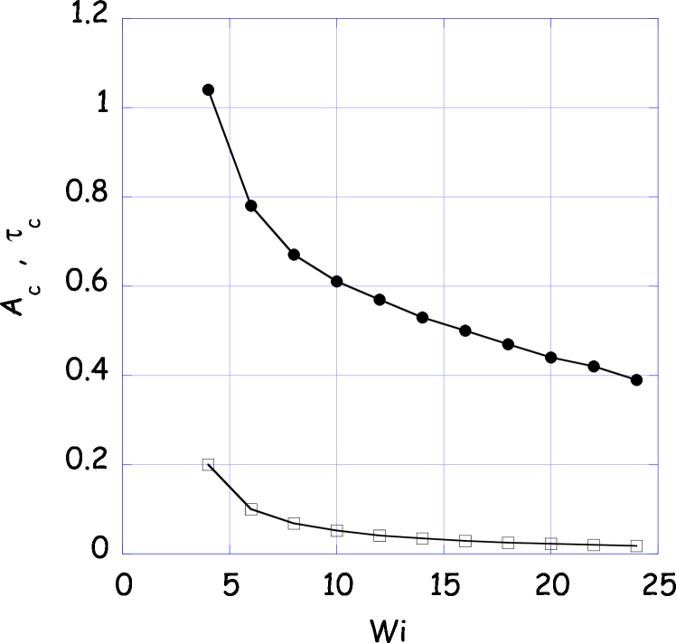
Figure 2: The critical amplitude and the critical stress for the case of planar Poiseuille flow of an UCM fluid, as determined from the weakly nonlinear expansion in this paper.

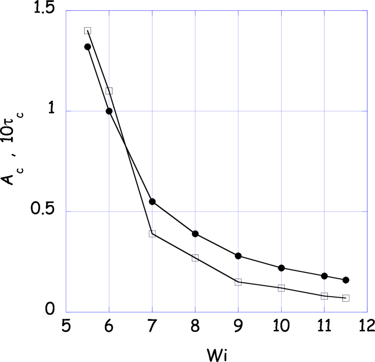
Figure 3: The critical amplitude and the critical stress for the cylindrical tube. Note that the critical values of $\tau_{23}/\tau_{23}^{\text{unp}}$ have been multiplied by 10 so as to be able to use the same scale.

Figure 4: Plot of the velocity field $\delta\vec{v}$ corresponding to the linear eigenmode of the cylindrical geometry with wavelength $\lambda=1.7R$ at ${\sf Wi}=8$. The basic flow profile is in the horizontal direction.

A few remarks concerning Figs. 2 and 3, which constitute the main result of our analysis, are in order:
     (i) Of course, our analysis is only based on an expansion to lowest nontrivial order in $A$; one may therefore wonder how much higher order nonlinear terms affect the result for $A_{\text{c}}$. Clearly, for small ${\sf Wi}$ where $A_{\text{c}}$ becomes of order unity, our results should not be trusted quantitatively: higher order (quintic) terms will change the answer (for the planare case they may even give rise to the existence of a true saddle-node bifurcation point). However, for large enough ${\sf Wi}$, our results can be trusted quantitatively. This is because the linear damping term $\text{Im}\,\omega$ becomes arbitrarily small at large ${\sf Wi}$ (it varies roughly as $\text{Im}\,\omega\sim 1/{\sf Wi}$), so that then the amplitude expansion for $A_{\text{c}}$ becomes nicely ordered.
     (ii) Since we have only determined the cubic nonlinearity in the equation, we can not say anything about the finite amplitude at which the instability will saturate. It is in fact questionable whether the saturation amplitude can be determined from any perturbative method. One hint that this might be possible to a reasonable approximation comes from the experiments of Bertola et al bonn1 ; bonn2 , which indicate that the amplitude of the perturbations of the extrudate just above ${\sf Wi}_{\text{c}}$ is rather small.
     (iii) The scale on the vertical axis is not arbitrary. In Figs. 2 and 3 we have plotted the size of the shear rate perturbation normalized to the shear rate at the wall in the unperturbed case. Using the equation

$$\left.\frac{\mbox{max}[\delta\tau_{rz}]}{\tau^{\text{unp}}_{rz}}\right|_{\text{wall}}=|C(1)A_{\text{c}}|,$$ (9)

which holds both for the cylindrical case and the planar case(with $r$ replaced by $y$), with $C(1)$ a numerical constant defined in Appendix  B, we show in Figs. 2 and 3 the ratio of the perturbed shear stress at the wall over the unperturbed shear stress at the wall, beyond which the flow is unstable. Note also the steep drop of the curve for ${\sf Wi}$ just above ${\sf Wi}_{\text{c}}$: for all practical purposes the transition is quite sharp.
     (iv) Our analysis also yields an idea of the value of $k$ of the mode with the smallest critical amplitude. For large enough ${\sf Wi}$ that our analysis can be trusted, we find typical values about twice the diameter of the slit or the tube both in the planar case and in the cylindrical case. A precise comparison has to be based on analyzing the frequency of the flow distortions measured at a fixed position, however, since the flow distorts upon exiting the die — see section IV.

I.4 Outline of the paper

We present our nonlinear analysis in some detail for various reasons. First of all, an amplitude analysis is normally used for problems with a true linear instability; the use of the method for cases like this one without a true instability involves some unusual nontrivial subtleties. Second, such an expansion makes use of left eigenvectors of the linear operator, whose behavior and boundary conditions are quite intricate and worth discussing. Third, the analysis we introduce may be of relevant to other visco-elastic flow problems as well.

In order to perform our weakly nonlinear analysis, we first have to reanalyze the linear stability problem. The essential results are summarized in section II. In order to facilitate comparison with the earlier work by Denn and coworkers denn2 ; denn1 , we write the equation for the stability eigenmodes in terms of the stream function, which satisfies a fourth order linear differential equation. The coefficients that we have (re)derived for this differential equation are given in appendices, and are the same as those given in the appendix of denn2 . A feature not discussed in the earlier work, however, is that there are various eigenmodes with different symmetries in the vertical direction for the planar case. In section III we first rewrite the linear eigenvalue problem in a form which is closer to the one usually found in derivations of an amplitude expansion ch ; walgraef . This is then followed by a discussion of the derivation of the cubic nonlinearity in the amplitude equation. A somewhat special feature of our approach that should be kept in mind is that normally amplitude expansions are used for an expansion around a true bifurcation point where a particular mode loses stability. Here the relevant linear modes are always weakly damped. This gives rise to some slight differences in the formulation.

II Linear stability analysis

After having formulated the problem for the planar case in the first subsection, we will summarize the main steps of the linear stability analysis in the second subsection. Detailed expressions for the coefficients are relegated to to appendices. The numerical results for the dispersion relation of the linear modes are presented in the last subsection.

II.1 Formulation of the problem

We would like to investigate the linear stability of polymeric flow between two plates, separate by a distance of $2d$, and through a cylinder of radius $R$. The direction orthogonal to the planes will be our $y$-direction, the direction of the unperturbed flow will be the $z$-direction — the advantage of this convention is that both in the planar and in the cylindrical geometry the mean flow is in the $z$-direction. From now on we take the flow two-dimensional by putting

$$v_{x}=0,~{}~{}~{}~{}~{}~{}v_{y,z}=v_{y,z}(y,z),$$ (10)

in the planar case and

$$v_{\theta}=0,,~{}~{}~{}~{}~{}~{}v_{r,z}=v_{r,z}(r,z).$$ (11)

in the cylindrical case. The first step is the derivation of an expression for the unperturbed flow:

$$\vec{v}^{\text{unp}}=(0,0,v^{\text{unp}}_{z}(y)),~{}~{}~{}~{}~{}~{}\vec{v}^{\text{unp}}=(0,0,v^{\text{unp}}_{z}(r)).$$ (12)

The next step is the perturbation of the unperturbed flow:

$$\vec{v} = \vec{v}^{\text{unp}}+(0,\delta v_{y}(y),\delta v_{z}(y))e^{i(kz-\omega t)},$$ (13)

$$\vec{v} = \vec{v}^{\text{unp}}+(\delta v_{r}(r),0,\delta v_{z}(r)),$$ (14)

$$\tau_{ij} = \tau_{ij}^{\text{unp}}+\delta\tau_{ij}e^{i(kz-\omega t)}.$$ (15)

We will keep the terms linear in $\delta\tau_{ij}$ and $\delta v$ and write the $\delta\tau_{ij}$ and $\delta v_{z}$ in terms of $\delta v_{y}$ (planar) or $\delta v_{r}$ (cylindrical) and its derivatives. This will give us a fourth order equations for $\delta v_{y}$ or $\delta v_{r}$. with boundary conditions. Solving this equation yields the dispersion relation $\omega(k)$; the imaginary part of $\omega$ determines the stability of the flow.

II.2 Equations and boundary conditions

II.2.1 The equations

The flow is taken to be incompressible, so that the conservation of mass equation becomes the incompressibility condition

$$\vec{\nabla}\cdot\vec{v}=0.$$ (16)

Moreover, as was already explained in the introduction, since we are interested in the zero Reynolds number limit, the Navier-Stokes equation, expressing conservation of momentum, reduces to the linear equation

$$-\vec{\nabla}p-\vec{\nabla}\cdot\vec{\vec{\tau}}=0.$$ (17)

We will take the curl of equation (17) to eliminate the pressure. This leaves us with an equation for the components of the stress tensor. The UCM model describes the stresses in the polymeric fluid bird :

$${\vec{\vec{\tau}}}+\lambda{\vec{\vec{\tau}}_{(1)}}=-\eta(\vec{\nabla}\vec{v}+(\vec{\nabla}\vec{v})^{\dagger}),$$ (18)

where the stress tensor $\vec{\vec{\tau}}_{(1)}$ is defined in the following way bird

$$\vec{\vec{\tau}}_{(1)} = \frac{D{\vec{\vec{\tau}}}}{Dt}-(\vec{\nabla}\vec{v})^{\dagger}\cdot\vec{\vec{\tau}}-\vec{\vec{\tau}}\cdot(\vec{\nabla}\vec{v}),$$ (19)

$$\frac{D}{Dt} = \frac{\partial}{\partial t}+\vec{v}\cdot\vec{\nabla}.$$ (20)

Eq. (18) illustrates that the UCM model is characterized by one time constant $\lambda$, which models the polymer relaxation time. The “upper convected derivative” $\vec{\vec{\tau}}_{(1)}$ is the simplest frame-independent formulation that implements this bird .

The UCM constitutive equation only models normal stress effects, no shear thinning. This is illustrated by the well-known fact that upon using the Ansatz (12) for $v^{\text{unp}}$, we find that the steady flow profile of a UCM fluid is still parabolic,

$$v^{\text{unp}}_{z}(y)=v_{\text{max}}\left[1-\left(\frac{y}{d}\right)^{2}\right],~{}~{}~{}~{}~{}\mbox{planar case},$$ (21)

where $v_{\text{max}}$ is the maximum velocity at the center line. Furthermore, for the stress tensor of the basic parabolic profile, one finds for the planar case simply

$$\tau^{\text{unp}}_{yz} = \tau^{\text{unp}}_{zy}=-\eta\frac{\partial v^{\text{unp}}_{z}(y)}{\partial y},$$ (22)

$$\tau^{\text{unp}}_{zz} = -2\eta\lambda\left(\frac{\partial v^{\text{unp}}_{z}(y)}{\partial y}\right)^{2}.$$ (23)

All other elements of $\tau^{\text{unp}}$ vanish. Note that $\tau_{zz}^{\text{unp}}$ is nonzero and proportional to the square of the shear — this is the normal stress effect.

The results in the cylindrical case are:

$$v^{\text{unp}}_{z}(r)=v_{\text{max}}\left[1-\left(\frac{r}{R}\right)^{2}\right],$$ (24)

and

$$\tau^{\text{unp}}_{rz} = \tau^{\text{unp}}_{zr}=-\eta\frac{\partial v^{\text{unp}}_{z}(r)}{\partial r},$$ (25)

$$\tau^{\text{unp}}_{zz} = -2\eta\lambda\left(\frac{\partial v^{\text{unp}}_{z}(r)}{\partial r}\right)^{2}.$$ (26)

The first step in a linear stability analysis is to linearize equation (18) to obtain expressions for the $\delta\tau$ which are linear in $\delta v$. At this stage, it is useful to introduce the stream function $\Phi$. Generally, the stream function is introduced by writing (for the planar case)

$$v_{y}=\frac{\partial\Phi}{\partial z},~{}~{}~{}~{}~{}~{}v_{z}=-\frac{\partial\Phi}{\partial y},$$ (27)

so that the incompressibility condition (16) is satisfied automatically. For linear perturbations of the form (13) we simply have $\Phi=\phi\;e^{i(kz-\omega t)}$, so that

$$\delta v_{y}(y)=ik\phi(y),\quad\quad\delta v_{z}(y)=-\frac{\partial\phi(y)}{\partial y}.$$ (28)

The stream function is slightly more complicated in the cylindrical case:

$$\frac{ik}{r}\phi(r)=\delta v_{r}(r),\quad-\frac{1}{r}\frac{\partial\phi(r)}{\partial r}=\delta v_{z}(r).$$ (29)

It is also convenient to introduce dimensionless variables

$$\quad{\hat{\omega}} = \frac{\omega d}{v_{\text{max}}},~{}~{}~{}~{}~{}~{}~{}~{}\quad\quad\hat{k}=kd,$$

$$\mbox{plane:}~{}~{}~{}~{}~{}\hat{z} = z/d~{}~{}~{}~{}~{}~{}~{}~{}~{}\quad\hat{t}=tv_{\text{max}}/d,$$ (30)

$$\xi = \frac{y}{d},$$

for the planar die, and

$$\quad{\hat{\omega}} = \frac{\omega R}{v_{\text{max}}},~{}~{}~{}~{}~{}~{}\quad\quad\hat{k}=kR,$$

$$\mbox{cylinder:}~{}~{}~{}\hat{z} = z/R~{}~{}~{}~{}~{}~{}~{}\quad\hat{t}=tv_{\text{max}}/R,$$ (31)

$$\xi = \frac{r}{R},$$

for the cylindrical die. For notational simplicity, we will rename $\hat{k}\Rightarrow k$, $\hat{z}\Rightarrow z$ and $\hat{t}\Rightarrow t$ and $\hat{\omega}\Rightarrow\omega$; it just means that we have to remember that all lengths are henceforth measured in units of $d$ or $R$, inverse lengths in units of $1/d$ or $1/R$, and times in unites of $d/v_{\text{max}}$ or $R/v_{\text{max}}$. The imaginary part of $\omega$ determines the linear stability of the flow; the flow is linearly stable if $\text{Im}\,\omega<0$. In order to facilitate comparison of our explicit expressions for the linear equation, given in appendix B, with the expressions of Rothenberger et al. denn2 , we also introduce their dimensionless number ${\sf S}$ denn2 ,

$${\sf S}=\frac{{\sf Wi}}{2}=\frac{2v_{\text{max}}\lambda}{d}.$$ (32)

Using definition (28) we obtain equations for the $\delta\tau$ in terms of $\phi(y)$. Equation (16) is always satisfied because of definition (28), equation (17) will give us a fourth order equation for $\phi(y)$ of the following form:

$$\phi^{\prime\prime\prime\prime}+\beta_{3}\phi^{\prime\prime\prime}+\beta_{2}\phi^{\prime\prime}+\beta_{1}\phi^{\prime}+\beta_{0}\phi=0,$$ (33)

where

$$\beta_{i}=\beta_{i}(k,{\sf S},\omega;\xi).$$ (34)

We used the symbolic manipulation program Maple to find the explicit expressions for the $\beta_{i}$: these expressions are the same as those given by Rothenberger et al. denn2 and can be found in the Appendix.

II.2.2 Boundary and symmetry conditions, planar case

The aim of the linear stability calculation is to determine $\omega(k)$ for fixed $k$ and ${\sf S}$, such that $\phi$ satisfies the usual stick boundary conditions:

$$v_{y}=0,\quad v_{z}=0\quad\mbox{at}\quad\xi=\pm 1.$$ (35)

For $\phi$ these boundary conditions translate into

$$\phi(\xi=\pm 1)=0,\quad\phi^{\prime}(\xi=\pm 1)=0.$$ (36)

Note that we have four boundary conditions, and a fourth order equation. At first sight, one might think that therefore the equation might have unique solutions for any $\omega(k)$. However, because of the linearity of the problem, if we find a solution $\phi(\xi)$, $C\phi(\xi)$ with $C$ an arbitrary complex constant is a solution of equation (33) as well. We eliminate this arbitrary degree of freedom by setting

$$\phi^{\prime\prime}(1)=1.$$ (37)

Since this eliminates two trivial degrees of freedom which do not affect the solution, it is now clear that for a given $k$ and ${\sf S}$, one or more unique branches of the complex quantity $\omega(k)$ will be fixed by the differential equation for $\phi$.

Because of the vertical symmetry of the problem, eigenfunctions will either be asymmetric or symmetric. In the first case the boundary conditions on the centerline are

$$\mbox{asymmetric:}~{}~{}~{}v_{y}=0,\quad v_{y}^{\prime\prime}=0\quad\mbox{at}\quad\xi=0,$$ (38)

which implies for $\phi(y)$

$$\mbox{asymmetric:}~{}~{}~{}\phi=0,\quad\phi^{\prime\prime}=0\quad\mbox{at}\quad\xi=0,$$ (39)

and in the second case the conditions are

$$\mbox{symmetric:}~{}~{}~{}v_{y}^{\prime}=0,\quad v_{y}^{\prime\prime\prime}=0\quad\mbox{at}\quad\xi=0,$$ (40)

which implies

$$\mbox{symmetric:}~{}~{}~{}\phi^{\prime}=0,\quad\phi^{\prime\prime\prime}=0\quad\mbox{at}\quad\xi=0.$$ (41)

We will explore the stability of both profiles below.

II.2.3 Boundary conditions, cylindrical case

We will take the usual stick boundary conditions $v_{r}=0$, $v_{z}=0$ at $\xi=\pm 1$. In the center we require $v_{r}=0$, $v_{z}$ finite. In terms of $\phi$ we have $\phi=0$, $\phi^{\prime}=0$ at $\xi=1$, and we choose $\phi^{\prime\prime}(1)=1$. We have to be careful in the origin, because of the $1/\xi$ terms in the equations for the $\beta_{i}$. The boundary conditions on $\vec{v}$ imply $\phi=0$, $\phi^{\prime}=0$ at $\xi=0$. In order to avoid numerical problems, we use a polynomial $\phi(\xi)=a_{2}\xi^{2}/2+a_{3}\xi^{3}/6$ for $\xi\in(0,0.01)$. At $\xi=0.01$ we match both solutions by imposing equality of $\phi$ and the first three derivatives.

II.2.4 Summary of the linear stability problem

In summary, we have to solve equation (33) with the condition (37) and the boundary conditions (36) and (39) for asymmetric modes or with the boundary conditions (36) and (41) in the case of symmetric modes. This means that we have to find the two complex parameters $\phi^{\prime\prime\prime}(1)$, $\omega(k)$, such that the conditions on the centerline are satisfied. In the cylindrical case we have to solve equation (33) with the boundary conditions discussed above. This means that we have to find the four complex parameters $\phi^{\prime\prime\prime}(1)$, $\omega$, $a_{2}$ and $a_{3}$ such that both solutions can be matched together.

II.3 Numerical results

II.3.1 The planar case

We have used a shooting program numrec to find the right parameters and to construct the eigenmodes corresponding to the two classes of boundary conditions. We present the results below for the range of $k$-values for which our program converged essentially to arbitrary precision. For larger values of $k$ the convergence becomes poorer, but since these larger values do not appear to be relevant for the nonlinear analysis of section III, we content ourselves with reporting simply the range where sufficient precision could be reached.

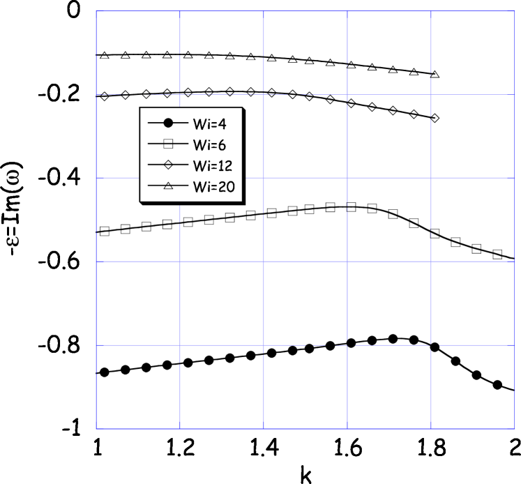
Figure 5: Dispersion relation for $\text{Im}\,\omega=-\varepsilon$ of the weakest damped asymmetric mode for ${\sf Wi}=4,6,12$ and $20$ in the planar case.

Fig. 5 shows the magnitude of the imaginary part of the eigenvalue $\omega$ of the asymmetric mode as a function of $k$ and for various ${\sf Wi}$. For all values of ${\sf Wi}$, $\text{Im}\,\omega<0$. As the temporal behavior of the modes is as $e^{-\varepsilon t}$, this confirms that the flow is linearly stable. Especially for large ${\sf Wi}$, $\varepsilon$ is very small, which means that the flow is only weakly stable. This is the reason that we also introduce the dimensionless temporal decay rate $\varepsilon=-\text{Im}\,\omega$, so that the positive quantity $\varepsilon$ is a small quantity for sufficiently large ${\sf Wi}$. This is very important, as the smallness of $\varepsilon$ will allow us to use an amplitude expansion in the next section: this expansion is based on an adiabatic approximation for the growth of the amplitude relative to the intrinsic oscillation of the waves with frequency $\text{Re}\,\omega$. Since the intrinsic frequency is of the order of unity in our dimensionless units, the condition for the amplitude expansion to work is that $\varepsilon\ll 1$.

We found a second asymmetric mode close to the first one reported in Fig. 5. This mode is slightly more damped than the first one. The two asymmetric modes are shown in Fig. 6. The symmetric mode lies between the two asymmetric modes, for, quite surprisingly, we have been able to show analytically that the symmetric mode obeys

$$\text{Im}\,\omega(k)=-\frac{2}{{\sf S}}\quad\Longleftrightarrow\quad\varepsilon=\frac{2}{{\sf S}}=\frac{4}{{\sf Wi}}.$$ (42)

so that for the the Weissenberg number ${\sf Wi}=8$ in Fig. 6 the damping rate of the symmetric mode is $\varepsilon=0.5$. For this mode the phase velocity $\text{Re}\omega(k)/k$ is extremely close to 1, but the precise value has to be determined numerically. Since the damping rates of all the three modes are very close, the above analytical result nicely shows that the damping rate of the modes becomes arbitrarily small for sufficiently large ${\sf Wi}=2{\sf S}$. Therefore, our amplitude expansion becomes self-consistent for sufficiently large ${\sf Wi}$.

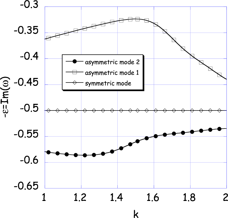
Figure 6: The dispersion relation for the two different linear asymmetric eigenmodes at ${\sf Wi}=8$ in the planar case, and the symmetric mode whose damping rate is given exactly by Eq. (42).

Once the eigenmode has been obtained numerically, one has the velocity and shear stress fields as a function of the coordinates. Fig. 8 of the introduction illustrates perturbed velocity field in the planar case for ${\sf Wi}=8$ and $k=1.5$.

Our nonlinear analysis in the next section will be based on using the asymmetric mode which is the weakest damped. The reason for not basing our expansion on the symmetric mode is twofold:
     (i) The symmetry of the velocity $v_{y}$ of this mode is such that it corresponds to a type of undulation mode between the plates, which does not generalize easily to the case of a cylindrical tube.
     (ii) The result that the eigenvalue $\omega(k)=(1+\delta)k-2i/{\sf S}$ for this mode, with $\delta$ a very small real quantity, implies that the factor $c(x)$ which appears at various places in the equations for the $\beta_{i}$ (see Appendix B), becomes very large near the center. Consequently, the components of $\tau$ become very large, almost singular, near the center.
     (iii) The asymmetric mode is the one least damped.

II.3.2 The cylindrical case

We now turn to the numerical results for the cylindrical case. Fig. 7 shows the magnitude of the imaginary part of the eigenvalue $\omega$ as a function of $k$ and for various ${\sf Wi}$. As in the planar case, all values of ${\sf Wi}$, $\text{Im}\,\omega<0$. As the temporal behavior of the modes is as $e^{-i\omega t}$, this again confirms that the flow is linearly stable; the decrease of $\varepsilon$ with increasing ${\sf Wi}$ again confirms that the linear stability becomes less and less with increasing flow velocity, roughly as $\varepsilon\sim 1/{\sf Wi}$.

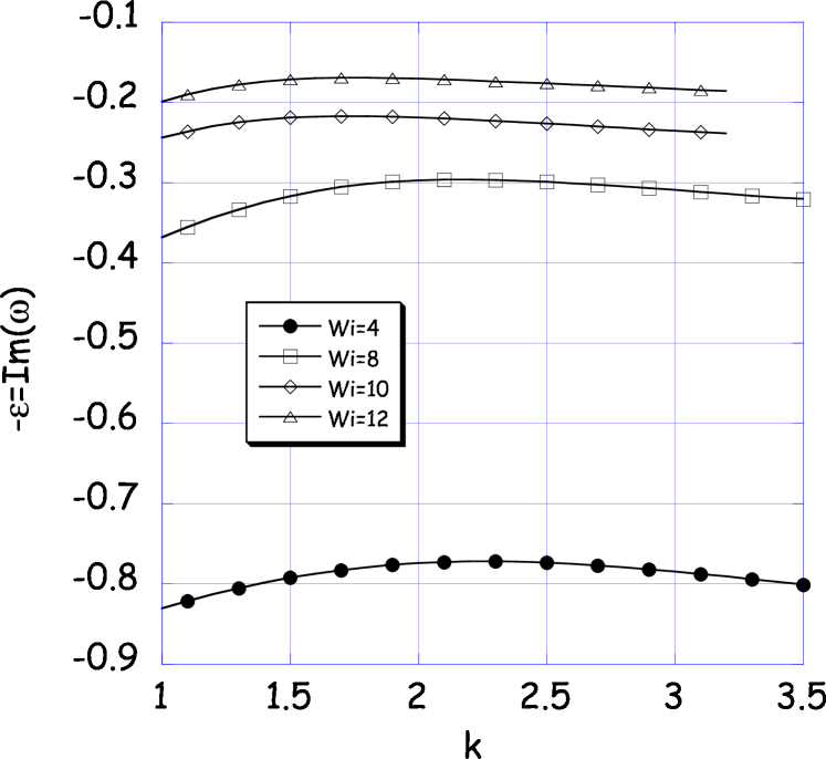
Figure 7: Dispersion relation for the cylindrical case for ${\sf Wi}=4,8,10$ and $12$.

Figure 8: Plot of the velocity field $\delta\vec{v}$ corresponding to the linear eigenmode mode of the planar slit geometry with wavelength $\lambda=4\pi/3$ at ${\sf Wi}=8$. The basic flow profile is in the horizontal direction.

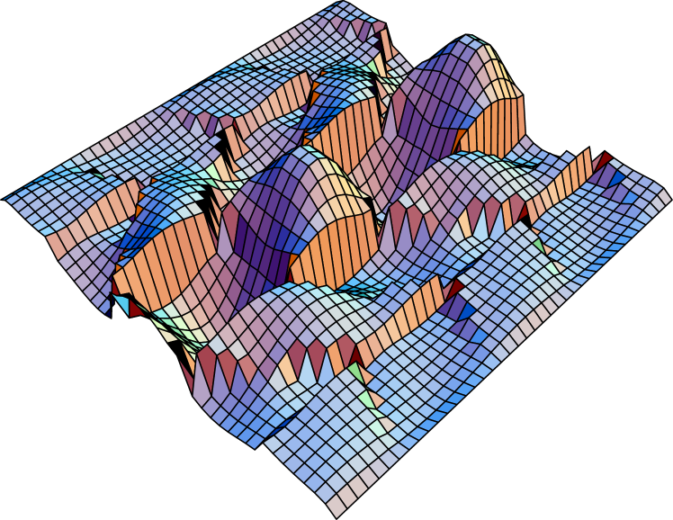
Figure 9: The data of Fig. 4 plotted differently. Here the component $\delta v_{z}$ is shown in a three-dimensional plot; it illustrates how the perturbation is largest at the center of the tube.

In Fig. 4 we already showed the velocity profile $\delta\vec{v}$ corresponding with the linear eigenmode with wavelength $\lambda=4\pi/3$ in the cylindrical case. Fig. 4 confirms that the same type of behavior is found in the planar case; the main difference is that in the cylindrical case, the mode is more confined close to the center of the tube (see also Fig. 9) than in the planar case. This is consistent with the fact that, as we will see in Section IV, the nonlinearly most unstable mode has a shorter wavelength in the cylindrical tube than in the case of the planar slit. In fact, the roll-type structure of the planar flow-profile is more evenly distributed over the whole cross-section, its qualitative appearance is closer than the cylindrical one to the flow pattern in the Taylor-Couette cell that according to the arguments of Groisman and Steinberg steinberg2 underlies the subcritical instability in that case.

III Nonlinear Analysis

We will start with an outline of the method that we use in the first section. As we shall see, in important ingredient that we need to obtain to determine certain solvability conditions is the solution of the linear adjoint operator. We will discuss the derivation of the adjoint problem in the sections III.2 and III.3. We finally discuss the numerical results in section III.4.

III.1 Outline of the structure of the amplitude expansion

In order to perform the nonlinear analysis it is convenient to rewrite the equations in a vector notation. We shall develop the framework for the planar case, and then indicate the changes in the cylindrical case at the end of this section.

Since we only consider perturbations which are independent of the coordinate $x$ in the planar case, the stress components $\tau_{xx}$, $\tau_{xy}$, and $\tau_{xz}$ are all zero, also in the nonlinear regime. We can therefore capture the nonzero fields in a five-component vector $V$ whose components are $\delta v_{y},\delta v_{z},\delta\tau_{22},\delta\tau_{23}$ and $\delta\tau_{33}$. Furthermore, we rewrite equations (16),(17) and (18) in the following form:

$${\mathcal{L}}V=N(V,V),$$ (43)

where ${\mathcal{L}}$ is the linear operator associated with the linear problem of section II, and $N(V,V)$ contains all the nonlinear terms. Thus the linear problem is simply ${\mathcal{L}}V=0$, and $N(V,V)$ contains only terms from the left hand side of equation (18); for the analysis below it is convenient to take $N$ symmetrized, so that $N(V_{1},V_{2})=N(V_{2},V_{1})$. Explicit expressions for $N(V,V)$ and ${\mathcal{L}}$ can be found in Appendix A.

Normally, an amplitude expansion is performed about the critical point where one of the modes is marginal (i.e., neither grows nor decays) for a particular value of the wavenumber $k$ ch ; walgraef . This critical wavenumber corresponds to a maximum of the linear dispersion relation. In the present case, the situation is not quite like this: the dispersion relation does not have a clear maximum, and the linear modes are always weakly damped. This difference is in practice not a great problem. First of all, we will not be interested in spatial variations of the envelope; instead, we just pick a particular mode $k$, and determine the important one for our analysis at a later stage (through the requirement that the threshold amplitude be minimal). It is therefore not necessary to expand about a maximum of the dispersion relation. Secondly, the amplitude expansion is based on an adiabatic decoupling of the fast and slow scales. In this problem, the fast scale is the period of the modes and the slow time scale is associated with the linear decay time of the modes. We saw in section II that in dimensionless units, the frequency of the modes is of order unity, while the damping rate $\varepsilon$ becomes much smaller than 1 for large enough ${\sf Wi}$. Thus, there is indeed a separation of times scales, and this is essentially all that is needed for the analysis below.

In fact, for readers experienced with amplitude expansions, we could essentially go ahead pretending we are expanding about a true critical point where the growth rate of one of the modes is zero, and then at the end add the linear damping term by hand. Nevertheless, we prefer to formulate the analysis more carefully by keeping the damping term as it stands.

A linear eigenmode of the equations is of the form

$$V_{0}(\xi,z,t;k,\omega) = \tilde{V}_{0}(\xi;k,\omega)\;e^{(ikz-i\omega t)}$$ (44)

$$= \tilde{V}_{0}(\xi;k,\omega)\;e^{(ikz-i\omega_{r}t)}\;e^{-\varepsilon t},$$

where we have introduced $\omega_{r}=\text{Re}\,\omega$. Of course, all components of $V_{0}$ can just be obtained directly from the results of the linear stability analysis of section II.

In an amplitude equation formalism, one can in general also allow for spatial variations of the amplitude on a slow scale. As we already remarked above, here we confine the analysis to the temporal evolution of a single mode $k$ and its harmonics. We do so for two reasons: First of all, it simplifies the analysis, secondly, our main goal is to determine whether there is a weakly nonlinear instability. Anticipating that we will find that there is one, there is then not much to be gained in allowing for slow spatial variations.

Our aim thus is to study the weakly nonlinear evolution in time of the amplitude $A$ of a single mode of the form

$$A(t)\;\tilde{V}_{0}(\xi;k,\omega)\;e^{(ikz-i\omega_{r}t)}+c.c.$$ (45)

Of course, such a single mode is not really a solution of the (weak) nonlinear equation, but the corrections are automatically accounted for in the amplitude equation formalism and are slaved to (45). We also note that because of the normalization (37), $\phi^{\prime\prime}(1)=1$, we have

$$\mbox{max}\left[\partial_{\xi}\delta v_{z}(\xi)|_{\text{wall}}\right]=2|A|$$ (46)

which, because in dimensionless units the shear rate at the wall in the unperturbed flow field equals 2, leads immediately to the the relation (8) between the maximum relative shear rate distortion at the wall and the amplitude $A$. Likewise the relation (9) between the amplitude $A$ and the maximum shear stress distortion at the wall follows from the explicit linearized dynamical equations. These identifications are important in translating our results to real values, as was already noted in section I.C and Fig. 2 and 3.

We want to know in particular whether the amplitude $A$ will grow or decay in time when the nonlinearities are taken into account. In the amplitude equation formalism, $A(t)$ is expected to depend only on the slow timescale $\varepsilon t$, but we have made this explicit, for reasons that become clear below. We have to keep track of the fact that the true zero mode of our linear operator ${\mathcal{L}}$ is $V_{0}$ as given in (44). This term includes the weakly damped exponential factor $e^{-\varepsilon t}$, and this term is not explicit in (45). The amplitude equation now proceeds by constructing the weakly nonlinear solution by writing ch ; walgraef

$$V=\varepsilon^{\frac{1}{2}}{V}^{s}_{0}+\varepsilon V_{1}+\varepsilon^{\frac{3}{2}}V_{2}+\cdots,$$ (47)

where $V^{s}_{0}$ is the real quantity defined as the sum

$${V}^{s}_{0}=B(T)V_{0}+B^{\star}(T)V_{0}^{\star},$$ (48)

and where in writing $B(T)$ we have anticipated that the amplitude $B$ varies on the slow timescale $T=\varepsilon t$. Note that the real combination ${V}^{s}_{0}$ is needed because the vector $V$ refers to real physical fields. Once we have derived the equation for $B$, comparison with (45) shows that we should make the association

$$A(t)\Longleftrightarrow\varepsilon^{\frac{1}{2}}B(T)e^{-\varepsilon t}.$$ (49)

The other terms in (47) are then precisely the corrections to the dominant mode which are necessary to construct a weakly nonlinear solution.

In the subsequent analysis, we have to keep in mind that $V_{0}$, with the temporal factor included, is the true zero eigenmode of the linear operator ${\mathcal{L}}$: The temporal derivatives in the linear operator in fact work explicitly on both temporal exponential factors in the expression (44) for $V_{0}$. When substituting the form (47) in the equations, we then also have to account for the time derivatives of $B(T)$. For a product term of the form $B(T)e^{-i\omega t}$ we then have

$$\frac{\partial\left(B(T)e^{-i\omega t}\right)}{\partial t}=B(T)\frac{\partial e^{-i\omega t}}{\partial t}+e^{-i\omega t}\varepsilon\frac{\partial B(T)}{\partial T},$$ (50)

which we can simply summarize by making the substitution $\partial_{t}\rightarrow\partial_{t}+\varepsilon\partial_{T}$ in all the time derivatives in the linear operator. Since only first order time derivatives enter the linear operator ${\mathcal{L}}$, we get an expansion of ${\mathcal{L}}$ of the form ${\mathcal{L}}={\mathcal{L}}_{0}+\varepsilon{\mathcal{L}}_{T}$.

The amplitude expansion now proceeds by substituting the expansions for ${\mathcal{L}}$ and (47) for $V$ in the nonlinear equation (43) and collecting the terms order by order in $\varepsilon$. For the first three orders in $\varepsilon$ we get:

$$\mbox{order}~{}\varepsilon^{\frac{1}{2}}:\hskip 71.13188pt{\mathcal{L}}_{0}{V}^{s}_{0} = 0,$$ (51)

$$\mbox{order}~{}\varepsilon^{1}:\hskip 71.13188pt{\mathcal{L}}_{0}V_{1} = N({V}^{s}_{0},{V}^{s}_{0}),$$ (52)

$$\mbox{order}~{}\varepsilon^{\frac{3}{2}}:~{}~{}~{}~{}~{}~{}~{}~{}~{}~{}{\mathcal{L}}_{0}V_{2}+{\mathcal{L}}_{T}{V}^{s}_{0} = N({V}^{s}_{0},V_{1}).$$ (53)

Equation (51) is satisfied identically, as it should, because ${V}^{s}_{0}$ is the sum of two terms with wavenumber $k$ and $-k$ which are both zero eigenmodes of ${\mathcal{L}}$. The components of the $V_{0}(\xi)$ follow from the numerical results for $\phi$ of section II. We can now solve equation (53) to find $V_{1}$. This gives us

$$V_{1}=B^{2}(T,t)\,e^{2i(kz+\omega_{r}t)-2\varepsilon t}\tilde{V}_{1}(\xi)+C(T)\,V_{0}~{}+~{}c.c.$$ (54)

where we have to find the vector $\tilde{V}_{1}(y)$ numerically, because N(V) contains only quadratic terms. The second term is allowed with arbitrary $C$, since $V_{0}$ is a zero mode of the linear operator ${\mathcal{L}}_{0}$; it will not be needed in the subsequent analysis. In principle, there would also have to be an additional $k=0$ term, but this term is identically zero for the case of the asymmetric boundary conditions of interest here. Once $V_{1}$ is known, we can proceed to Eq. (53); in this equation, the operator ${\mathcal{L}}_{T}$ works on $B(T)$ and its complex conjugate only: we can write the equation as

$${\mathcal{L}}_{0}V_{2}+(V_{0}\;{\mathcal{L}}_{T}B+V^{*}_{0}\;{\mathcal{L}}_{T}B^{*})=N(V_{0},V_{1}).$$ (55)

This equation determines the time derivative of $B$ through a solvability condition: since the operator ${\mathcal{L}}_{0}$ has a right zero mode, it can be solved if and only if the other two terms in the equation are orthogonal to the left zero mode of ${\mathcal{L}}_{0}$ ch ; walgraef . This requirement gives us the desired equation of ${\rm d}B/{\rm d}T$. To make this explicit, we first have to define the adjoint problem and an inner product.

We define a space of 5-dimensional vector functions of the three variables $\xi,z$ and $t$,

$$\Omega=\{f:R^{3}\rightarrow R^{5}:f=\tilde{f}(\xi,t)e^{i(kz-\omega_{r}t)}\}.$$ (56)

The components of the functions $f$ satisfy the physical boundary conditions discussed in section II. Furthermore, an inner product $I$ on $\Omega$ is defined:

$$I(w,f)=\frac{1}{2}\int_{-1}^{1}\!\!\!{\rm d}\xi\;\frac{2\pi}{k}\int_{0}^{\frac{2\pi}{k}}\!\!\!{\rm d}z\;\frac{2\pi}{\omega_{r}}\int_{0}^{\frac{2\pi}{\omega_{r}}}\!\!\!{\rm d}t\otimes$$

$$\otimes\sum_{i=1}^{5}w^{\star}_{i}(\xi,z,t)f_{i}(\xi,z,t).$$ (57)

On this space of functions, an adjoint operator ${\mathcal{L}}_{0}^{\dagger}$ is defined such that

$$I(w,{\mathcal{L}}_{0}f)=I({\mathcal{L}}_{0}^{\dagger}w,f)$$ (58)

for every function $f$ in $\Omega$. Because the adjoint operator is obtained through partial integrations with respect to $\xi$, the requirement that (58) does not yield any boundary terms from these partial integrations yields the appropriate boundary conditions for the functions $g$ in the adjoint space. We will state these explicitly for our case in section III.2.

Let $W_{0}$ be the zero mode of ${\mathcal{L}}_{0}^{\dagger}$. The solvability condition applied to (55) then becomes

$$I(W_{0},N(V^{s}_{0},V_{1})-V_{0}{\mathcal{L}}_{T}B-V^{\star}_{0}B^{\star})=0.$$ (59)

Let us focus on the term with $B$; if we write

$$W_{0}=\sum_{m\in\mathbb{Z}}g_{m}(y,T,t)e^{im(kz-\omega_{r}t)}$$ (60)

we see that we only need the term with $m=1$, since the inner product in (59) is seen to vanish for all other terms after the $z$-integration is performed. For the same reason, we only need the terms which are proportional to $e^{i(kz-\omega_{r}t)}$ from $N(V_{0},V_{1})$. Using this we obtain the following equation for the derivative of $B$:

$$\frac{1}{2}\int_{-1}^{1}\!\!\!{\rm d}\xi\;\left(W_{0}^{\star},-{\mathcal{L}}_{T}B+|B|^{2}BN(V_{0}^{\star},V_{1})\right)=0.$$ (61)

The complex conjugate of this equation is obtained from analyzing the term with $B^{*}$ in (59).

In (59), we have used the approximation that $\varepsilon$ is sufficiently small that we are allowed to write

$$\int_{0}^{\frac{2\pi}{\omega_{r}}}\!\!\!{\rm d}t\;B(T)e^{-\varepsilon t}\,(\cdot)=B(T)e^{-\varepsilon t}\int_{0}^{\frac{2\pi}{\omega_{r}}}\!\!\!{\rm d}t\;(\cdot).$$ (62)

This is nothing but the usual adiabaticity assumption. As we have shown in section II, this approximation is justified for large ${\sf Wi}$. We can summarize the Eq. (61) in the form

$$\partial_{T}B=c_{0}|B|^{2}B,$$ (63)

where $c_{3}$ is a complex quantity which is obtained from working out the two inner product terms. We can now translate this result back into the lowest order nonlinear equation for the amplitude $A$. Upon combining (49), and (63), we finally get

$$\partial_{t}A=-\varepsilon A+c_{3}|A|^{2}A,$$ (64)

which is nothing but Eq. (6) of the introduction in dimensionless units. As discussed there, the sign of the real part of $c_{3}$ determines whether or not we are dealing with a subcritical bifurcation.

In the following sections the boundary conditions of the adjoint problem are derived, and we then proceed to solve adjoint problem and to determine $c_{3}$.

The framework laid out above can be extended rather easily to the case of the cylindrical tube. In that case we consider axially symmetric perturbations only, so that both $\tau_{\theta r}$ and $\tau_{\theta z}$ vanish; note, however, that $\tau_{\theta\theta}$ is nonvanishing in this case. The vector $V$ therefore now has six components, $\delta v_{r},\delta v_{z},\delta\tau_{rr},\delta\tau_{rz},\delta\tau_{\theta\theta}$ and $\delta\tau_{zz}$. Apart from this change, the structure of the expansion is essentially the same, except for trivial changes like the fact that the first integration in (57) should now be taken over the two-dimensional scaled radial coordinate $\xi$.

III.2 The adjoint operator and associated boundary conditions

In this section we will calculate the components of the adjoint operator ${\mathcal{L}}_{0}^{\dagger}$ using the defining equation (58). We will follow again the planar case, and indicate the major changes for the cylindrical case at the end an in the appendices. Writing $V=(v_{1},\ldots,v_{5})$ and $W=(w_{1},\ldots,w_{5})$ we have

$${\mathcal{L}}_{0}V=\left(\begin{array}[]{ccccc}\partial_{y}v_{1}+\partial_{z}v_{2}\\ \partial_{y}\partial_{z}v_{3}+(\partial_{z}^{2}-\partial_{y}^{2})v_{4}-\partial_{y}\partial_{z}v_{5}\\ Cv_{1}+Av_{3}\\ Dv_{1}+Ev_{2}+Bv_{3}+Av_{4}\\ Fv_{1}+Gv_{2}+2Bv_{4}+Av_{5}\end{array}\right).$$ (65)

The various functions and coefficients in this expression are given in Appendix A. We will illustrate the structure of the calculation by analyzing two terms of $I(W,{\mathcal{L}}_{0}V)$, and simply state the results for the other terms. One term we get is $w_{3}^{\star}Av_{3}$:

$$\int\!\!w_{3}^{\star}Av_{3} = \int\!\!w_{3}^{\star}\left(1+\partial_{t}+\frac{{\sf S}}{2}v_{z}^{0}(\xi)\partial_{z}\right)v_{3},$$ (66)

$$= \int\!\!\left(1-\partial_{t}-\frac{{\sf S}}{2}v_{z}^{0}(\xi)\partial_{z}\right)w_{3}^{\star}v_{3}$$

$$~{}~{}~{}+\frac{{\sf S}}{2}\int\!\!\partial_{z}(w_{3}^{\star}v_{3})+\int\!\!\partial_{t}(w_{3}^{\star}v_{3}).$$

Both integrals on the last line vanish, the first one because the integrand is a partial $z$-derivative of a term which is periodic in $z$, the second one because the integrand is a partial $t$-derivative of a term which is periodic in $t$. Thus we simply obtain

$$\int\!\!\!w_{3}^{\star}Av_{3}=\int\!\!\!\left(1-\partial_{t}-\frac{{\sf S}}{2}v_{z}^{0}(y)\partial_{z}\right)w_{3}^{\star}v_{3}.$$ (67)

In short: we pick up a minus sign for every partial integration and in performing the partial integrations we get, in general, boundary terms which have to vanish. In the above example, the boundary terms trivially vanished because of the periodicity of the terms with respect to $t$ and $z$, but the partial integrations with respect to $\xi$ do not automatically vanish. In particular, from the various terms we get the following boundary conditions:

$$w_{3}^{\star}v_{1}(1)-w_{3}^{\star}v_{1}(-1) = 0,$$

$$w_{4}^{\star}v_{1}(1)+w_{4}^{\star}v_{1}(-1) = 0,$$

$$w_{4}^{\star}v_{2}(1)-w_{4}^{\star}v_{2}(-1) = 0,$$

$$w_{5}^{\star}v_{2}(1)+w_{5}^{\star}v_{2}(-1) = 0,$$

$$w_{1}^{\star}v_{1}(1)-w_{1}^{\star}v_{1}(-1) = 0.$$ (68)

and

$$w_{2}^{\star}\partial_{z}v_{3}(1)-w_{2}^{\star}\partial_{z}v_{3}(-1) = 0,$$

$$w_{2}^{\star}\partial_{y}v_{4}(1)-w_{2}^{\star}\partial_{y}v_{4}(-1) = 0,$$

$$\partial_{y}w_{2}^{\star}v_{4}(1)-\partial_{y}w_{2}^{\star}v_{4}(-1) = 0,$$

$$w_{2}^{\star}\partial_{z}v_{5}(1)-w_{2}^{\star}\partial_{z}v_{5}(-1) = 0.$$ (69)

The first set of conditions (III.2) is always satisfied, because $V$ satisfies the boundary conditions of the original problem: $v_{1}(\pm 1)=v_{y}(\pm 1)=0$ and $v_{2}(\pm 1)=v_{z}(\pm 1)=0$. By setting $w_{2}=0$ at $\xi=\pm 1$, we have only one condition left of the second set:

$$\partial_{\xi}(1)w_{2}^{\star}v_{4}(1)-\partial_{\xi}w_{2}(-1)^{\star}v_{4}(-1)=0.$$ (70)

In order to understand how many boundary conditions we need to impose, it is good to realize that the operator $\mathcal{L}$ actually works on physical, and hence real functions; thus, we need the real part of this combination to be zero. Thus, we can still choose the phases of both amplitudes: we use this freedom to set the phase difference between the adjoint solution $W_{0}$ and the solution $V$ such that the combination $w_{2}^{\star}v_{4}(1)$ becomes purely imaginary. This shows us that if we impose

$$\text{Re}\left(\partial_{\xi}w_{2}^{\star}|_{1}v_{4}(1)-\partial_{\xi}w_{2}^{\star}|_{-1}v_{4}(-1)\right)=0$$ (71)

all conditions are satisfied for physical functions. We can give all $w_{i}$ in terms of $w_{2}$ and its derivatives. This gives a fourth order equation for $w_{2}$ which we solve using a shooting method. We will discuss the appropriate symmetry conditions in the next section.

In the cylindrical case, we need $w_{2}$ to be bounded. In the present case, this can be achieved by putting $w_{2}(0)=0$, $w_{2}^{\prime\prime}(0)=0$. These conditions are satisfied if we expand $w_{2}(\xi)=a_{1}\xi+\frac{1}{6}a_{3}\xi^{3}$, for $0<x<0.01$. Furthermore we can set $a_{1}=1$ to eliminate the degree of freedom we have. This leaves us with one shooting parameter, $a_{3}$. We again have the boundary condition that $w_{2}$ vanishes on the wall, $w_{2}(1)=0$. We choose $a_{3}$ such that this condition is satisfied.

III.3 Symmetry of the solution and the adjoint solution

As we discussed in section section II, the linear planar mode that we investigate is asymmetric, which means that its symmetry is

$$\tilde{V}(\xi)=(odd,even,even,odd,even)$$ (72)

which can be verified, see Appendix B. For the adjoint solution we have also have two zero modes with different symmetry,

$$\tilde{W}^{(1)}_{0}(\xi)=(even,odd,even,odd,even),$$ (73)

and

$$\tilde{W}^{(2)}_{0}(\xi)=(odd,even,odd,even,odd).$$ (74)

It turns out that for our choice of the linear mode (72), the second mode $W^{(2)}_{0}$ does give a solvability condition. This can be seen as follows. Only the last three components of the vector $V$ contain a derivative $\partial_{T}$. Thus only the overlap of the third, fourth and fifth component of $W_{0}$ and $V_{0}$ come in; because of the symmetry of the opposite symmetry of the components, all these integral vanish. The same holds for the $N$-term, and hence the solvability condition is trivially satisfied. As a result, $W^{(1)}_{0}$ is the adjoint zero mode which gives the nontrivial boundary condition. The oddness of the component $w_{2}$ is then guaranteed by taking

$$w_{2}(0)=0,\quad w_{2}^{\prime}(0)=1,\quad w_{2}^{\prime\prime}(0)=0.$$ (75)

These conditions, together with the boundary condition at $\xi=\pm 1$ completely fixes the adjoint zero mode. As with the linear problem discussed in section II, we solve the differential equation together with the boundary conditions with a shooting method.

In the cylindrical case, we have just one single mode, also for the adjoint problem; the boundary conditions that we already derived above for the cylindrical case are completely analogous to the above boundary conditions (75).

III.4 Numerical Results

In summary, the nonlinear term $c_{3}$ whose real part governs the weak nonlinear stability is obtained numerically as follows. We first solve the fourth order equation for the stream function $\phi_{0}$, derived in section II. This gives us the components of the vector $V_{0}(\xi)$. A second routine of this program generates the term $N(V_{0},V_{0})$ too. A second program calculates the stream function $\phi_{1}$ of the inhomogeneous equation (52) from which we obtain the components of the vector $V_{1}(y)$. A third program solves the adjoint problem and gives the vector $W_{0}$. Because we have $W_{0}\sim e^{i(kz-\omega_{r}t)},V_{0}\sim e^{i(kz-\omega_{r}t)}$ and $V_{1}\sim e^{2i(kz+\omega_{r}t)}$ we have trivial $z$ and $t$ integrations in the inner product (61). The $\xi$-integration is done numerically from $0$ to $1$ because of symmetry. This then gives us the coefficient $c_{3}$.

We first discuss the cylindrical case. In Fig. 10 we plot the value of the critical amplitude $A_{\text{c}}(k)$, determined from $c_{3}$ by Eq. (7), as a function of the wavenumber $k$ for three different values of the Weissenberg number. The curves illustrate that for ${\sf Wi}>{\sf Wi}_{\text{c}}$ there is a band of wavenumbers where $\text{Re}\,c_{3}>0$ and that hence there is, in our approximation, a critical amplitude beyond which the flow is unstable. The sharp rise of the critical amplitude at the edges of the bands shown in Fig. 10 are close to the edges of the band where $\text{Re}\,c_{3}\to 0$. Note also that for ${\sf Wi}=7.5$, the critical value still has a rather sharp minimum near $k=4$, but that for increasing values of ${\sf Wi}$ the bottom of the band flattens rapidly. For decreasing values of ${\sf Wi}$, especially when ${\sf Wi}$ approaches about 5, the band likewise sharpens; we will see this from a different perspective below.

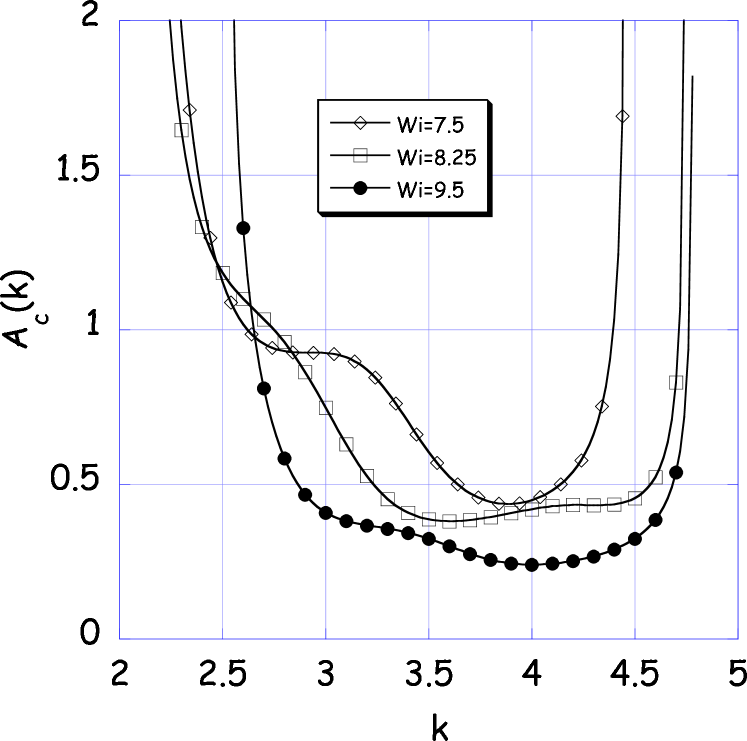
Figure 10: The value of the critical value $A_{\text{c}}$ as a function of the wavenumber $k$ for three different values of the Weissenberg number ${\sf Wi}$ for the case of the cylinder.

Fig. 10 also shows the behavior of the critical amplitude $A_{\text{c}}(k)$ as a function of $k$ shows rather complicated structure. For ${\sf Wi}=7.5$ there is a plateau in the critical value of $A_{\text{c}}(k)$ around $k=2.7$; upon increasing ${\sf Wi}$, this plateau shifts and disappears, whereas the absolute minimum of the curve shifts to smaller $k$ values while a new minimum develops at larger $k$. Already at ${\sf Wi}=8.25$, the two minimum almost correspond to the same values of $A_{\text{c}}$, but for slightly larger ${\sf Wi}$ the minimum at larger $k$ value becomes the absolute minimum. This is further illustrated in Fig. 11, where we plot the values of $k$ corresponding to the absolute minima of the curves, as well as the values corresponding to an amplitude 1.1 times the minimum value, as a function of ${\sf Wi}$. The figure illustrates that between ${\sf Wi}\approx 6.5$ and ${\sf Wi}\approx 8$, the minimum of the curve shifts to smaller $k$ values, but that around ${\sf Wi}\approx 8$ a local minimum at higher $k$-values becomes the absolute minimum.

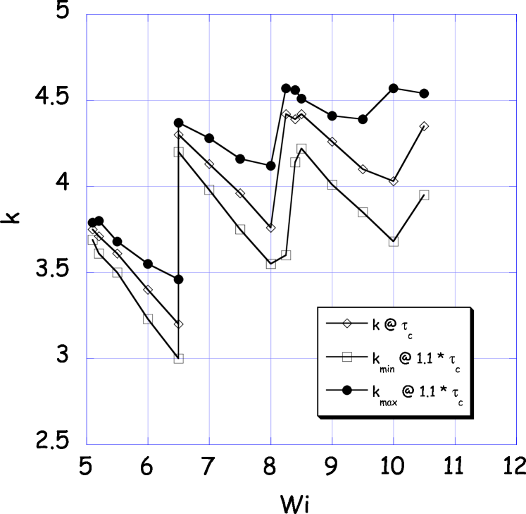
Figure 11: The value of $k$ corresponding to the minimum value of the curves in Fig. 10 as a function of ${\sf Wi}$, and the values of $k$ at which the amplitude $A$ is 1.1 times the minimum value. The jumps of the curves are due to fact that a curve of $A_{\text{c}}$ as a function of $k$ has several minima.

As explained in section II.2.4, our normalization is such that $A$ is the maximum perturbation in the shear rate at the wall over one wavelength, divided by the shear rate at the wall of the unperturbed parabolic profile [See Eq. (8)]. Upon increasing ${\sf Wi}$, the minimum values of the curves, which were already plotted in Fig. 3, quickly decrease. As we already mentioned in the introduction, we have also analyzed the critical value for the relative shear stress perturbation at the wall beyond which the flow is unstable [see Eq. (9)]. The data for this ratio as a function of $k$ for the same values of the Weissenberg number as in Fig. 10 are shown in Fig. 12. There are several important things to note about this figure. First of all, the curves of the critical shear stress perturbation have just one minimum, contrary to those for the critical shear perturbation, and secondly, the values for the critical shear stress perturbation are typically a factor ten smaller than those for the critical shear. As Fig. 12 shows, for ${\sf Wi}=9.5$ a perturbation of about 1% in the wall shear stress is sufficient to render the flow unstable. This is why in Fig. 3 the values of the critical shear stress amplitude (the values corresponding to the minima of the curves in Fig. 12) are multiplied by 10 to draw them on the same scale as $A_{\text{c}}$. Finally, we note that the edge of the band of unstable shear stress perturbations $\tau$ is the same as the edge of the band of unstable shear perturbations — this is simply due to the fact that the edge of the band is marked by the point where $\text{Re}\,c_{3}=0$.

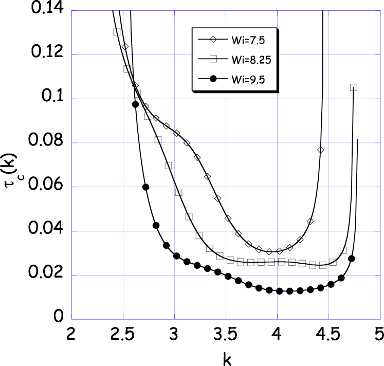
Figure 12: The values of the dimensionless shear stress $\tau$ beyond which the flow is unstable in the cylinder, as a function of $k$ for the same three values of ${\sf Wi}$ as in Fig. 10.

In Fig. 13 we plot the band in which modes are nonlinearly unstable beyond some critical value as a function of ${\sf Wi}$. This figure clearly illustrates that the width of the band vanishes at ${\sf Wi}={\sf Wi}_{\text{c}}\approx 5$, since below this values $\text{Re}\,c_{3}<0$ for all $k$. This figure is somewhat reminiscent of the so-called “Busse balloon” of Rayleigh-Bénard convection ch , but one should keep in mind that the interpretation is slightly different as we are dealing with a subcritical (inverted) bifurcation. Thus, the regions marked “Stable” indicate the regions in the diagram where the perturbations with a wavenumber $k$ in that region are nonlinearly stable in our approximation. The basic Poisseuille flow profile is, however, nonlinearly unstable at all ${\sf Wi}_{\text{c}}$ to modes whose wavenumber lies in the band marked “Unstable”. In reality, we expect that the flow pattern will settle to some kind of stable nonlinear behavior dominated by modes in this band.

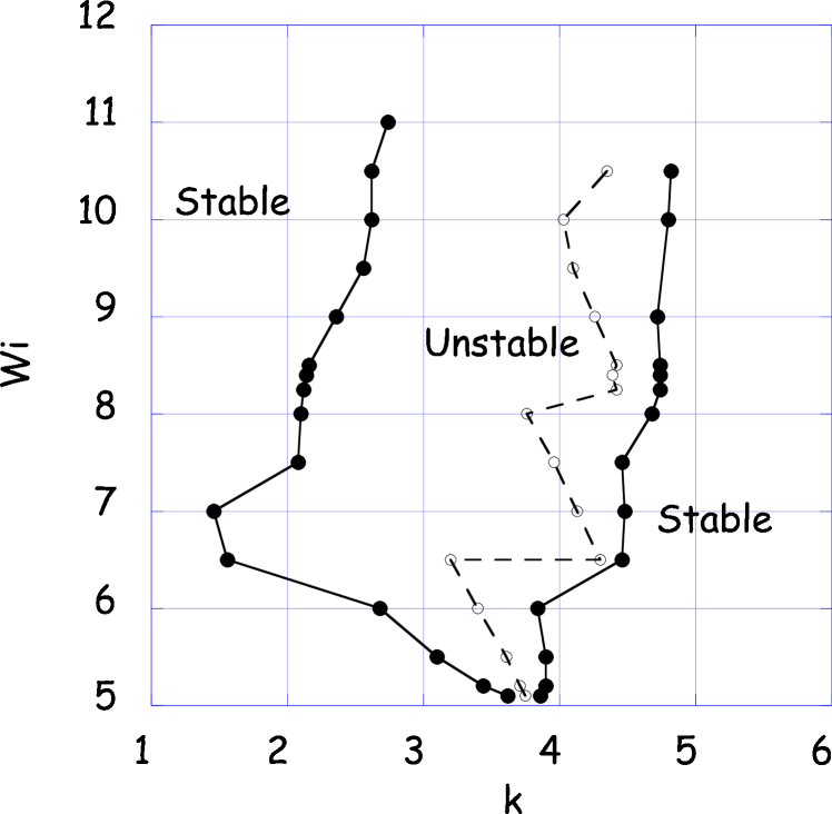
Figure 13: Plot of the width of the $k$-band where the corresponding modes render the basic cylindrical Poiseuille flow nonlinearly unstable. The dashed line indicates the $k$-value of the mode which is most unstable to shear perturbations, i.e. the minimum of the curves plotted in Fig. 10.

Although the band of unstable modes widens toward small $k$-values for ${\sf Wi}$ between 6 and 7.5 — a feature which is related to the plateau in Fig. 10 for ${\sf Wi}=7.5$ — at flow rates (Weissenberg numbers) about 50% beyond the critical value, the band of unstable wavenumbers ranges from just over 2 to a value somewhat larger than 4. Although with our expansion to cubic order in the amplitude we can not probe the stable nonlinear patterned flow regime nor the nonlinear selection of the wavenumber (it need not correspond to the most unstable mode), it seems reasonable to assume that the wavenumbers of the pattern in the tube will lie in the range identified by Fig. 13.

Because near ${\sf Wi}_{\text{c}}$ the critical amplitude is relatively large, and again because we have only expanded up to cubic order, one has to interpret our results near ${\sf Wi}_{\text{c}}$ with caution. Nevertheless, our results appear to identify the location of the saddle-node bifurcation to nontrivial flow patterns near ${\sf Wi}_{\text{c}}\approx 5$. Since the band of unstable modes in this limit is very small, it appears likely that if one follows the nontrivial flow pattern down to this value, its wavenumber is should be close to the value where the band in Fig. 13 closes,

$${\sf Wi}\approx{\sf Wi}_{\text{c}}\approx 5:~{}~{}\Longrightarrow~{}~{}~{}~{}k\approx 3.75,$$ (76)

since the basic profile is then nonlinearly stable to perturbations with wavenumber that differs significantly from this value. In dimensional units, this implies for the wavelength $\Lambda$ of the pattern

$${\sf Wi}\approx{\sf Wi}_{\text{c}}\approx 5:~{}~{}~{}~{}~{}~{}\Lambda\approx 2\pi R/3.75\approx 1.7\,R.$$ (77)

It is important to keep in mind that $k$ is the wavenumber inside the cylindrical tube. If the (near)periodic flow and stress patterns inside the tube indeed cause the surface undulations that are the first stage leading to melt fracture outside the tube at larger flow rates, then one should keep in mind that $k$ is not the wavenumber of these surface undulations. For, the polymer extrudate swells upon leaving the tube, and the flow velocity profile of the polymer becomes essentially constant after leaving the tube. A better way to compare our theory with measurements on the extrudate is therefore to compare the (dominant) frequency of the undulations: since no oscillations will disappear at the outlet of the tube, the frequency measured inside the tube must be equal to the frequency with which the the extrudate width oscillates after flowing out of the tube bonn1 . Of course, the frequency of the oscillations on the nonlinear flow branch corresponding to the solid line in Fig. 1 can not be obtained precisely from our expansion; assuming that the nonlinearities do not change this frequency too much, we estimate it from our results for the linear modes. From our analysis of the linear eigenmodes in section II we find that the dimensionless frequency $\text{Im}\,\omega$ of the modes is to a very good approximation (better than to a percent or so) given by

$$\text{Im}\,\omega=k-0.93/{\sf Wi}.$$ (78)

This result implies that for large Weissenberg numbers, the phase velocity $\text{Im}\,\omega/k$ approaches 1. Since according to (31) we measure velocities in units of $v_{\text{max}}$, this means that the periodic stress pattern moves essentially with the maximum velocity of the flow in the large Weissenberg limit. This indicates that the linear mode more and more concentrated near the axis of the tube for large ${\sf Wi}$. The above result gives as an estimate for the frequency $f$ in dimensional units

$$f=v_{\text{max}}(k-0.93/{\sf Wi})/(2\pi R)$$ (79)

Finally, using that we expect the transition to occur at ${\sf Wi}_{\text{c}}\approx 5$ and $k\approx 3.75$, and that for the unperturbed (parabolic) profile of a UCM fluid $v_{\text{max}}=2v_{\text{av}}$ with $v_{\text{av}}$ the average flow velocity in the tube, our estimate for the frequency at the transition becomes

$$\mbox{at transition:}~{}~{}~{}f\approx 1.13\,v_{\text{av}}/R.$$ (80)

It is important to realize that this estimate is based on the assumption that the frequency (or phase velocity) does not get renormalized significantly by the nonlinearities. This is maybe not unreasonable near threshold, where the amplitude of the periodic modulation of the pattern will be smallest (keep in mind that since we are dealing with a subcritical bifurcation, the amplitude near threshold remains finite).

Especially further above threshold, we expect the renormalization of the frequency to be significant. Although this can not be calculated from our first nontrivial nonlinear term in the amplitude expansion, we can reasonably estimate the frequency at values of ${\sf Wi}$ of the order of 50 to 100% above threshold, say, as follows. As we noted above, in this range, the band of unstable wavenumbers $k$ ranges from just over 2 to about 4.5 (See Fig. 14). It is unlikely that the range of wavenumbers will change drastically due to nonlinear interactions, since in according to our calculations outside this range both the linear and the cubic term in the amplitude expansion are stabilizing. On the other hand, the frequency of oscillations, if one studies the pattern in a fixed lab frame, will get strongly renormalized: once the pattern gets well developed, we expect (but have no proof) that the nonlinearly modulated profile moves with the average speed $v_{\text{av}}$ rather than with the maximum speed of the unperturbed parabolic profile (keep in mind that in linear order, the periodic linear eigenmode does not affect the average speed, as it averages out to zero over one wavelength, but that this does not remain true in nonlinear order). Which particular wavenumber will be selected nonlinearly (or whether in fact a well-defined sharp wavenumber will be selected nonlinearly in a carefully controlled experiment) we do not know, but with the assumption that it lies in the unstable band $k_{\text{min}}<k<k_{\text{max}}$ and that it moves with the average speed, we get the following estimate for the dimensional frequencynotefreq

$$\frac{k_{\text{min}}v_{\text{av}}}{2\pi R}\lesssim f\lesssim\frac{k_{\text{min}}v_{\text{av}}}{2\pi R},$$ (81)

which gives

$$\frac{0.3\,v_{\text{av}}}{R}\lesssim f\lesssim\frac{0.72\,v_{\text{av}}}{R}.$$ (82)

We finally turn to a brief discussion of our results for the case of a planar slit. The main difference between the cylindrical and planar case is that in the latter case, the coefficient $\text{Re}\,c_{3}$ is always found to be positive. This is also illustrated by Figs. 14 and 15, which show that in the case of the planar slit there is no finite band of nonlinearly unstable wavenumbers for the critical shear rate (Fig. 14) and critical shear stress (Fig. 15) as a function of $k$. Note also that in both cases these curves just have a single minimum, contrary to what we found for the cylindrical tube. As a result of this, the wavenumber corresponding the minimum of the amplitude shear rate critical value $A_{\text{c}}$ now decreases smoothly with ${\sf Wi}$, see Fig. 16.

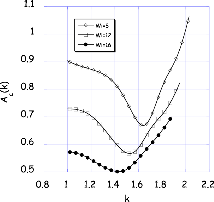
Figure 14: Plot of the critical amplitude $A_{\text{c}}$ as a function of $k$ in the planar case for three different values of ${\sf Wi}$.

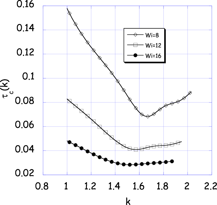
Figure 15: Plot of the critical amplitude $\tau_{\text{c}}$ as a function of $k$ in the planar case for three different values of ${\sf Wi}$.

The absence of a finite band of wavenumbers and of a value of ${\sf Wi}$ below which $\text{Re}\,c_{3}<0$ for all $k$ (as in the cylindrical case), appears to have fewer practical implications than one might expect at first sight. After all, the overall behavior of the minimal value of the critical amplitudes as a function of ${\sf Wi}$ shows quite the same behavior as in the case of the cylinder, compare Figs. 2 and 3: upon decreasing ${\sf Wi}$, the critical values rapidly decrease below ${\sf Wi}\approx 5$. As we have stressed before, our expansion ceases to be valid in this regime where $A_{\text{c}}$ becomes of order unity. We expect that in reality there is also a true saddle-node bifurcation point where the branch ends in the case of planar Poiseuille flow; possibly, our results indicate that in the planar case the corresponding critical value ${\sf Wi}_{\text{c}}$ is lower than in the cylindrical case. However, our results do imply that it is difficult to make a prediction for the wavenumber near this (presumed) critical value than in the case of the cylinder. Nevertheless, since the wavenumber of the mode whose threshold to nonlinear instability is smallest is about 1.8, it seems reasonable to expect for the dimensional wavelength near threshold

$${\sf Wi}\approx{\sf Wi}_{\text{c}}:~{}~{}~{}~{}~{}~{}~{}~{}\Lambda\approx 2\pi d/1.8\approx 3.5\,d$$ (83)

where the width of the slit equals $2d$. Like for the case of flow in a pipe, according to our linear results the phase velocity is very close to the maximum velocity at the center line between the plates, so the above result for the most likely wavelength near threshold yields a frequency of about $2.7\,v_{\text{av}}/d$. However, since we do not find a finite band of unstable modes above threshold, it is difficult to determine the range of frequencies expected further above threshold, even though we do expect here too that the patterns move roughly with the average velocity.

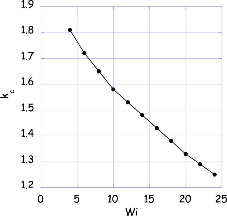
Figure 16: The value $k_{c}$ of the wavenumber corresponding to the minimum of $A_{\text{c}}$ as a function of $k$ for the case of planar Poiseuille flow.

IV Discussion and outlook

In this article we have shown that for the simplest model of a polymer fluid with normal stress effects, the UCM model, Poiseuille flow through a planar channel or cylindrical tube becomes weakly nonlinearly unstable for Weissenberg numbers somewhat larger than unity. Stated differently, since the UCM model only includes the essential normal stress effect, we find that the nonlinear flow instability is characterized by the Weissenberg number only, and the phenomenon appears to be very robust in that almost any more complicated polymer fluid model that includes normal stress effects will exhibit the same instability in the same range of Weissenberg numbers. We presented evidence in meulenbroek ; bonn1 that this instability yields an intrinsic route to melt fracture behavior in the absence of other mechanisms such as stick-slip phenomena.

One should also keep in mind that our expansion is only carried out to lowest order in the nonlinearity, so one may wonder about the robustness of these results as long as higher order terms in the expansion are unknown. Investigations of these issues for Couette flow and Poiseuille flow are underway and will be reported in due course.

The critical Weissenberg number we find is a factor 10 larger than the values for which Atalik and Keunings keunings observed self-sustained quasi-periodic oscillations in their numerical simulations of Poiseuille flow. The two results are not necessarily inconsistent however: while all of our calculations apply to the UCM model, their simulations were done for the Oldroyd-B model, with a viscosity ratio of $10^{-3}$ and Reynolds number ${\sf Re}=0.1$. Moreover, Atalik and Keunings added a stress diffusion term to their equations to improve numerical stability. Further analysis is clearly necessary to investigate the effects of these differences — a detailed comparison of the simulations with the amplitude expansion results for one and the same model, is called for.

Just above the onset of a well-defined linear (or “supercritical”) instability threshold, the wavelength of the pattern is well-defined: upon approach of the threshold, the wavenumber of the pattern approaches the wavenumber $k_{c}$ at which the instability sets in. Here, however, it is more difficult to draw sharp conclusions about the wavelength of the pattern close to onset. First of all, our expansion can not be fully trusted quantitatively for Weissenberg numbers of the order of ${\sf Wi}_{\text{c}}$, as the damping rate is large there, not small as is needed in our method. This technical caveat aside, one should keep in mind that once the instability sets in the nonlinear flow behavior which will develop can not be addressed by our expansion method. Hence it is difficult to rule out the possibility of nonlinear interaction terms changing the velocity of the pattern in the die to a value different from the one we have assumed, namely the average flow velocity $v_{\text{a}}$. If on the other hand the flow pattern stabilizes in some weakly nonlinear regime, then one would expect its wavenumber to be close to the onset value we calculate and the frequency to be close to the one we have estimated in Eq. (80). As a rule of thumb, the wavelength of the undulations of the extrudate is typically about twice the diameter of the die.

In conclusion, our nonlinear analysis establishes the nonlinear flow instability essentially beyond reasonable doubt and predicts onset values which are consistent with those reported experimentally denn1 ; pahl ; bonn1 ; bonn2 . Moreover, the hypothesis of highly similar subcritical behavior in Taylor-Couette geometries steinberg1 ; steinberg2 and Poiseuille flow (and hence possibly melt fracture) is fully confirmed by our calculations. Indeed, the similarity between the flow field perturbation shown in Fig. 8 and the roll-type pattern which Groisman and Steinberg have argued gives rise to the subcritical nature of the instability steinberg2 in Taylor-Couette flow is striking. From this perspective, the only difference between the two cases is that the general mechanism larson ; shaqfeh2 ; pakdel that in visco-elastic flows the curvature of the streamlines makes the flow linearly unstable is operative in Taylor-Couette cells but obviously not in Poiseuille flow. Nonlinearly, the two flows appear to be much more closely connected. From this perspective, the evidence for “turbulence without inertia” steinbergturb ; larsonturb as a result of these elastic effects is intriguing.

V Acknowledgement

WvS would like to thank Daniel Bonn for stimulating his interest in the polymer flow problem and Daniel Bonn for numerous discussions. Moreover, he is grateful to the LPS of the ENS in Paris for its hospitality and to the French Ministère des affaires étrangères and French Ministère de l’éducation nationale, de la recherche et de la technologie, for a Descartes-Huygens award which made frequent visits to Paris possible.

Appendix A Explicit expressions for the operator $\mathcal{L}$ and the nonlinear term $N$

In this section we give the expressions for the operators ${\mathcal{L}}$ and $N$ from the equation

$${\mathcal{L}}V=N(V,V)$$ (84)

in the planar case and the cylindrical case in dimensional form.

For the planar case we have

$${\mathcal{L}}=\left(\begin{array}[]{ccccc}\partial_{y}&\partial_{z}&0&0&0\\ 0&0&\partial_{y}\partial_{z}&\partial_{z}^{2}-\partial_{y}^{2}&-\partial_{y}\partial_{z}\\ C&0&A&0&0\\ D&E&B&A&0\\ F&G&0&2B&A\\ \end{array}\right),$$

where the operators $A-G$ are defined in the following way:

$$A = 1+\lambda\partial_{t}+\lambda v_{z}^{0}(y)\partial_{z},$$ (85)

$$B = -\lambda\frac{\partial v_{z}^{0}(y)}{\partial y},$$ (86)

$$C = 2(\eta\partial_{y}-\lambda\tau^{0}_{yz}(y)\partial_{z}),$$ (87)

$$D = \eta\partial_{z}-\lambda\left(\tau^{0}_{zz}(y)\partial_{z}-\frac{\partial\tau^{0}_{yz}(y)}{\partial y}\right),$$ (88)

$$E = \eta\partial_{y},$$ (89)

$$F = \lambda\partial_{y}\tau^{0}(y)_{zz},$$ (90)

$$G = -2\lambda(\tau^{0}_{zz}(y)\partial_{z}+\tau^{0}_{yz}(y)\partial_{y})+2\eta\partial_{z}$$ (91)

and

$$N_{1} = 0,$$ (92)

$$N_{1} = 0,$$ (93)

$$N_{3} = \lambda\left(-v_{y}\frac{\partial\tau_{yy}}{\partial y}-v_{z}\frac{\partial\tau_{yy}}{\partial z}\right.$$ (94)

$$\hskip 56.9055pt\left.+2(\frac{\partial v_{y}}{\partial y}\tau_{yy}+\frac{\partial v_{y}}{\partial z}\tau_{yz})\right),$$

$$N_{4} = \lambda\left(-v_{y}\frac{\partial\tau_{yz}}{\partial y}-v_{z}\frac{\partial\tau_{yz}}{\partial z}+\frac{\partial v_{z}}{\partial y}\tau_{yy}\right.$$ (95)

$$\hskip 56.9055pt\left.+\frac{\partial v_{y}}{\partial z}\tau_{zz}\right),$$

$$N_{5} = \lambda\left(-v_{y}\frac{\partial\tau_{zz}}{\partial y}-v_{z}\frac{\partial\tau_{zz}}{\partial z}+2(\frac{\partial v_{z}}{\partial y}\tau_{yz}\right.$$ (96)

$$\hskip 56.9055pt\left.+\frac{\partial v_{z}}{\partial z}\tau_{zz})\right).$$

For the cylindrical case we get

$$L=\left(\begin{array}[]{cccccc}\frac{1}{r}+\partial_{r}&\partial_{z}&0&0&0&0\\ 0&0&\partial_{z}(\partial_{r}+\frac{1}{r})&0&M&-\partial_{r}\partial_{z}\\ B&0&A&0&0&0\\ C&D&E&A&0&0\\ F&0&0&0&A&0\\ G&H&0&I&0&A\\ \end{array}\right),$$ (97)

where the operators $A-M$ are defined in the following way:

$$A = 1+\lambda\partial_{t}+\lambda v_{z}^{0}(r)\partial_{z},$$ (98)

$$B = 2\eta\left(\partial_{r}+\lambda\frac{\partial v_{z}^{0}(r)}{\partial r}\partial_{z}\right),$$ (99)

$$C = \eta\left(\partial_{z}-\lambda\frac{\partial^{2}v_{z}^{0}(r)}{\partial r^{2}}-\frac{\lambda}{r}\frac{\partial v_{z}^{0}(r)}{\partial r}\right.$$ (100)

$$\hskip 28.45274pt+\left.2\lambda^{2}\left(\frac{\partial v_{z}^{0}(r)}{\partial r}\right)^{2}\partial_{z}\right),$$

$$D = \eta\partial_{r},$$ (101)

$$E = -\lambda\frac{\partial v_{z}^{0}(r)}{\partial r},$$ (102)

$$F = \frac{2\eta}{r},$$ (103)

$$G = -4\eta\lambda^{2}\,\frac{\partial v_{z}^{0}(r)}{\partial r}\,\frac{\partial^{2}v_{z}^{0}(r)}{\partial r^{2}},$$ (104)

$$H = 2\eta\partial_{z}+\eta\lambda\frac{\partial v_{z}^{0}(r)}{\partial r}\left(2\partial_{r}+4\lambda\frac{\partial v_{z}^{0}(r)}{\partial r}\partial_{z}\right),$$ (105)

$$I = -2\lambda\frac{\partial v_{z}^{0}(r)}{\partial r},$$ (106)

$$K = -\frac{1}{r}\partial_{r}+\frac{1}{r^{2}}-\partial^{2}_{r}+\partial^{2}_{z}$$ (107)

$$M = -\frac{1}{r}\partial_{z}$$ (108)

and the vector $N$ has components

$$N_{1} = 0$$ (109)

$$N_{2} = 0$$ (110)

$$N_{3} = \lambda\left(-v_{r}\frac{\partial\tau_{rr}}{\partial r}-v_{z}\frac{\partial\tau_{rr}}{\partial z}+2\frac{\partial v_{r}}{\partial r}\tau_{rr}\right.$$ (111)

$$\hskip 56.9055pt\left.+2\frac{\partial v_{r}}{\partial z}\tau_{rz}\right)$$

$$N_{4} = \lambda\left(-v_{r}\frac{\partial\tau_{rz}}{\partial r}-v_{z}\frac{\partial\tau_{rz}}{\partial z}+\frac{\partial v_{z}}{\partial r}\tau_{zz}\right.$$ (112)

$$\hskip 56.9055pt\left.+\frac{\partial v_{z}}{\partial r}\tau_{rz}-\frac{v_{r}}{r}\tau_{rz}\right)$$

$$N_{5} = \lambda\left(-v_{r}\frac{\partial\tau_{\theta\theta}}{\partial r}-v_{z}\frac{\partial\tau_{rz}}{\partial z}\right.$$ (113)

$$\hskip 56.9055pt\left.+2\frac{v_{r}}{r}\tau_{\theta\theta}\right)$$

$$N_{6} = \lambda\left(-v_{r}\frac{\partial\tau_{zz}}{\partial r}-v_{z}\frac{\partial\tau_{zz}}{\partial z}\right.$$ (114)

$$\hskip 42.67912pt\left.+2(\frac{\partial v_{z}}{\partial r}\tau_{rz}+\frac{\partial v_{z}}{\partial z}\tau_{zz})\right).$$

Appendix B Explicit expressions for the coefficient $\beta_{i}$

The coefficients of the equation for the streamfunction in the planar case:

$$\beta_{0} := k^{2}(k^{2}+i\,k{\sf S}+2k^{2}{\sf S}^{2}\xi^{2}-6i\,C(\xi)k{\sf S}^{3}\xi^{2}$$ (115)

$$-i\,C(\xi)k{\sf S}+3C(\xi){\sf S}^{2}+6i\,C(\xi)^{2}k{\sf S}^{3}\xi^{2}$$

$$+4C(\xi)^{2}{\sf S}^{4}k^{2}\xi^{4}+2C(\xi)^{2}k^{2}{\sf S}^{2}\xi^{2}),$$

$$\beta_{1} := 2k^{2}{\sf S}\xi(i\,k-2{\sf S}+4C(\xi){\sf S}-2i\,C(\xi)k{\sf S}^{2}\xi^{2}$$ (116)

$$-i\,C(\xi)k-2C(\xi)^{2}{\sf S}+2i\,C(\xi)^{2}k{\sf S}^{2}\xi^{2}),$$

$$\beta_{2} := -k(3i\,{\sf S}+2k+2k{\sf S}^{2}\xi^{2}-3i\,C(\xi){\sf S}$$ (117)

$$-4C(\xi)k{\sf S}^{2}\xi^{2}+2C(\xi)^{2}k{\sf S}^{2}\xi^{2});$$

$$\beta_{3} := 2i\,k[{\sf S}\xi(-1+C(\xi)),$$ (118)

$$C(\xi) := 2/(2+i\,k{\sf S}(1-\xi^{2}-c)),$$ (119)

where the complex dimensionless coefficient $c=\omega/k$ is used by Rothenberger et al denn2 .

The coefficients of the streamfunction in the cylindrical case are

$$\beta_{0} := k^{3}(k-4i\,C(\xi){\sf S}^{3}\xi^{2}+4k[{\sf S}^{4}\xi^{4}C(\xi)^{2}$$ (120)

$$+2k{\sf S}^{2}\xi^{2}C(\xi)^{2}+4i\,C(\xi)^{2}{\sf S}^{3}\xi^{2}$$

$$+2k\xi^{2}{\sf S}^{2}),$$

$$\beta_{1} := (-2{\sf S}^{2}\xi^{4}k^{2}+2k^{2}\xi^{2}-2i\,k^{3}\xi^{4}{\sf S}C(\xi)$$ (121)

$$-3+4{\sf S}^{2}\xi^{4}C(\xi)k^{2}+2i\,k^{3}\xi^{4}{\sf S}$$

$$-2C(\xi)^{2}{\sf S}^{2}\xi^{4}k^{2}+4i\,k^{3}\xi^{6}C(\xi)^{2}{\sf S}^{3}$$

$$-4i\,k^{3}\xi^{6}C(\xi){\sf S}^{3})/(\xi^{3}),$$

$$\beta_{2} := -(-3-4{\sf S}^{2}\xi^{4}C(\xi)k^{2}+2C(\xi)^{2}{\sf S}^{2}\xi^{4}k^{2}$$ (122)

$$+2k^{2}\xi^{2}+2{\sf S}^{2}\xi^{4}k^{2})/(\xi^{2}),$$

$$\beta_{3} := 2(-i\,k\xi^{2}{\sf S}-1+i\,{\sf S}\xi^{2}C(\xi)k)/\xi,$$ (123)

$$C(\xi) := 1/(1+i/2k{\sf S}(1-\xi^{2}-c)).$$ (124)

References

- (1) R. B. Bird, R. C. Armstrong and O. Hassager Dynamics of Polymeric Liquids (Wiley, New York, 1987).
- (2) R. Rothenberger, D. H. McCoy and M. M. Denn, Trans. Soc. Rheol. 17, 259 (1973).
- (3) T. C. Ho and M. M. Denn, J. Non-Newtonian Fluid Mechanics 3, 179 (1978).
- (4) K. Atalik and R. Keunings, J. Non-Newtonian Fluid Mech. 102, 299 (2002).
- (5) B. Yesilata, Fluid Dyn. Res. 31, 41 (2002).
- (6) M. M. Denn, Issues in visco-elastic fluid mechanics, Annu. Rev. Fluid Mech. 13, 13-34 (1990).
- (7) M. M. Denn, Annu. Rev. Fluid Mech. 28, 129 (1996).
- (8) M. Pahl, W. Gleissle and H.-M. Laun, Praktische Rheologie der Kunststoffe und Elastomere (VDI verlag, 1991).
- (9) B. Meulenbroek, C. Storm, V. Bertola, C. Wagner, D. Bonn, and W. van Saarloos, Phys. Rev. Lett. 90 , 024502 (2003).
- (10) V. Bertola, B. Meulenbroek, C. Wagner, C. Storm, A. Morozov, W. van Saarloos and D. Bonn, Phys. Rev. Lett. 90, 114502 (2003).
- (11) V. Bertola, C. Wagner and D. Bonn (unpublished).
- (12) R. G. Larson, E. S. G. Shaqfeh and S. J. Muller, J. Fluid Mech. 218, 573-600 (1990).
- (13) Y. L. Joo and E. S. G. Shaqfeh, Phys. Fluids A 3, 1691 (1991).
- (14) Y. L. Joo and E. S. G. Shaqfeh, Phys. Fluids A 4, 524-540 (1992).
- (15) N. Phan-Tien, J. Non-Newtonian Fluid Mech. 13, 325-340 (1983).
- (16) N. Phan-Tien, J. Non-Newtonian Fluid Mech. 17, 37-44 (1985).
- (17) E. S. G. Shaqfeh, Annu. Rev. Fluid Mech. 28, 129-185 (1996).
- (18) P. Pakdel and G. H. MacKinley, Phys. Rev. Lett. 77, 2459 (1996).
- (19) A. Groisman and V. Steinberg, Phys. Rev. Lett. 78, 1460 (1997).
- (20) A. Groisman and V. Steinberg, Phys. Fluids 10, 2451 (1998).
- (21) R. Sureshkumar, A. N. Beris and M. Avgousti, Proc. Roy. Soc. Lond. A 447, 135-153 (1994).
- (22) D. D. Joseph, in: Hydrodynamic Instabilities and the Transition to Turbulence, H. L. Swinney and J. P. Gollub, eds. (Springer, Berlin, 1981).
- (23) P. Huerre and M. Rossi, in: Hydrodynamics and Nonlinear Instabilities, G. Godrèche and P. Manneville, eds. (Cambridge University Press, Cambridge, 1998).
- (24) S. Grossmann, Rev. Mod. Phys. 72, 603 (2000).
- (25) C. L. Pekeris and B. Shkoller, J. Fluid Mech. 29, 31 (1967).
- (26) L. M. Hocking, K. Stewartson and J. T. Stuart, J. Fluid Mech. 51, 705 (1972).
- (27) Th. Herbert, in Proceedings of the AGARD symposium on Laminar-Turbulent Transitions, (1977).
- (28) There is an important lesson from the earlier work on planar Poiseuille flow: expansions to higher order in the amplitude do not appear to help to capture the nonlinear branch in the case of Newtonian fluids. Th. Herbert, AIAA Journal 18, 243 (1980) has extended the expansion of hocking through terms of order 15 in the amplitude expansion, but the series does not appear to capture the physically relevant regime of Reynolds numbers and amplitudes.
- (29) S. J. Chapman, Subcritical transition in channel flows, to appear in J. Fluid Mech.
- (30) M. C. Cross and P. C. Hohenberg, Rev. Mod. Phys. 65, 851 (1993).
- (31) D. Walgraef, Spatio-temporal Pattern Formation (Springer, Berlin 1996).
- (32) W. H. Press, B. P. Flannery, S. A. Teukolsky and W. T. Vetterling, Numerical Recipes, (Cambridge University Press, Cambridge, 1986).
- (33) Note that the band extends to slightly smaller values at flow rates about 50% beyond threshold. In this range, the lower estimate for the frequency might be better replaced by .
- (34) A. Groisman and V. Steinberg, Nature 405, 53 (2000).
- (35) R. Larson, Nature 405, 27 (2000).