Non linear excess conductivity of Bi₂Sr₂Ca_n-1Cu_nO_2n+4+x ($n$ = 1, 2) thin films

Abstract

The suppression of excess conductivity with electric field is studied for Bi₂Sr₂Ca_n-1Cu_nO_2n+4+x ($n$ = 1, 2) thin films. A pulse-probe technique is used, which allows for an estimate of the sample temperature. The characteristic electric field for fluctuations suppression is found well below the expected value for all samples. For the $n=1$ material, a scaling of the excess conductivity with electric field and temperature is obtained, similar to the scaling under strong magnetic field.

I Introduction

High-$T_{c}$ superconductors exhibit strong superconducting fluctuations at the superconducting temperature, as a result of the high ratio of the transition temperature to the condensation energy - essentially due to their short coherence length. Such fluctuations have been extensively studied in the weak and strong fluctuation limits (respectively the Gaussian and the critical regime). There is now a rising interest in the possibility to suppress superconductivity by the application of an electric field, and the study of the electric field dependence of the fluctuations appears as a first step towards this goal. Early theoretical work has focused on the reduction of the excess conductivity in the Gaussian regime, by the application of a transport current approaching the depairing current (non linear conductivity). The electric field dependence of the Aslamazov-Larkin termaslamazov68 was obtained in Refs. hurault69 ; schmidt69 ; tsuzuki69 ; gorkov70 , and the one of the additional ’anomalous’ Maki-Thompson termthompson70 in Ref. maki71 . Experimental results on Al films demonstrated the suppression of fluctuations by the electric field in the isotropic two-dimensional limitkajimura70 ; kajimura71 . The theory, based on a Langevin equation for the order parameter, was extended to below $T_{c}$ in Ref. kajimura71b . Later, several works considered the contribution of the interaction of fluctuations in the critical region and, recently, the expression for the fluctuation conductivity in the transition region was revisited and the similarity of the results with those obtained for the broadening of the transition under a strong magnetic field was pointed out (see Ref. puica03 and refs therein). Such experiments on high-$T_{c}$ superconductors are difficult, as they require high current densities, which generally induce an uncontrolled heating of the sample. As a result, only few experimental works have investigated the effect of the electrical field on the resistive transition of the cuprates. In Ref. soret93 , a field-induced crossover between a three-dimensional and two-dimensional behavior was reported for a YBa₂Cu₃O_7-x single crystal, in the temperature range $\epsilon=(T-T_{c})/T_{c}<2\;10^{-2}$. In Ref. gorlova95 , the non-linear resistivity in the range $0<\epsilon<7\;10^{-2}$ was used to obtained the characteristic depairing field of Bi₂Sr₂CaCu₂O_8+x single crystal. It was found to be about 10 times smaller than the expected value and its temperature dependence was clearly different from the $\epsilon^{3/2}$ dependence predicted in Ref. schmidt69 .

In this contribution, we compare the excess conductivity suppression for this system with the one in Bi₂Sr₂CuO_6+x, where the investigation of temperature intervals as large as $-0.2<\epsilon<0.6$ was possible due to an electrical critical field more than one order of magnitude smaller.

II Experiment

The measurements were carried out on Bi₂Sr₂Ca_n-1Cu_nO_2n+4+x ($n$ = 1, 2) epitaxial, c-axis oriented thin films. They were grown on heated SrTiO₃ substrates, by reactive rf sputtering with an oxygen rich plasma (Ref. li93 and refs therein). After deposition of typically 2500 Å thick films, Au contacts were sputtered, and the samples were patterned in the four contact transport geometry, with a current carrying strip of typical width and length ($L$) of 80 $\mu$m and 200 $\mu$m. The annealing of the samples at low temperature was used to set the doping state, which was determined from the normal state resistivity temperature dependencekon00 . The thin film with $n=2$ (sample II) was overdoped. A thin film with $n=1$ was studied for two different doping states: an overdoped one (sample Ia) and an underdoped one (sample Ib). Two other samples with $n=1$ (samples Ic and Id), respectively close to optimal doping and strongly overdoped, were also investigated. The sample parameters are summarized in Table 1.

The resistivity in the limit of vanishing current density was obtained using a 10 $\mu$A ac current and a lock-in amplifier detection. The investigation for large current densities was carried out using the pulsed current technique. The current pulses where 10 $\mu$s long, with a repetition rate $\tau=10^{-4}$ and the maximum current value was 100 mA. Both the voltage on a reference resistor fed with the measuring current and the one on the sample, after amplification by home-made amplifiers, were recorded, using a $2.5$ MHz, 16 bits digital acquisition card. The measurement of the resistance, obtained from the ratio of the two voltages, was linear within 0.3% over the current range. The non linearity was corrected from the raw measurements. Evaluating the temperature increase due to the measuring current is crucial for the high current density transport experiments, as an apparent decrease of the excess conductivity with current may occur, due to the sample temperature increase only. A reliable determination of the non linear excess conductivity requires a method for measuring the sample temperature. For this purpose, we modified the technique to a ’pulse-probe’ one: after the completion of the main 10 $\mu$s pulse with current density $J$ and the measurement at the end of this pulse, a probe pulse with current $J_{s}\ll J$ is performed immediately after. A typical secondary current pulse was $J_{s}\simeq J/50$. Neglecting the sample heating by current $J_{s}$, the value of the resistance during the secondary pulse provides a measure for the sample temperature about 1 $\mu$s after the main pulse, using the ac resistivity data as a thermometer. Such a method does not, however, catch the fast temperature relaxation which occurs between the main and the probe pulses. This relaxation, with a typical relaxation time in the ns rangecarr90 , may be estimated as $\Delta T\simeq R\,i^{2}/A\,\lambda$, where $A$ is the sample surface and $\lambda\simeq 10^{7}$ WK^-1m^-2 is the boundary conductance, yielding $\Delta T\simeq 0.01$ K and 0.1 K for samples with $n=1$ and $n=2$ respectively.

III results and discussion

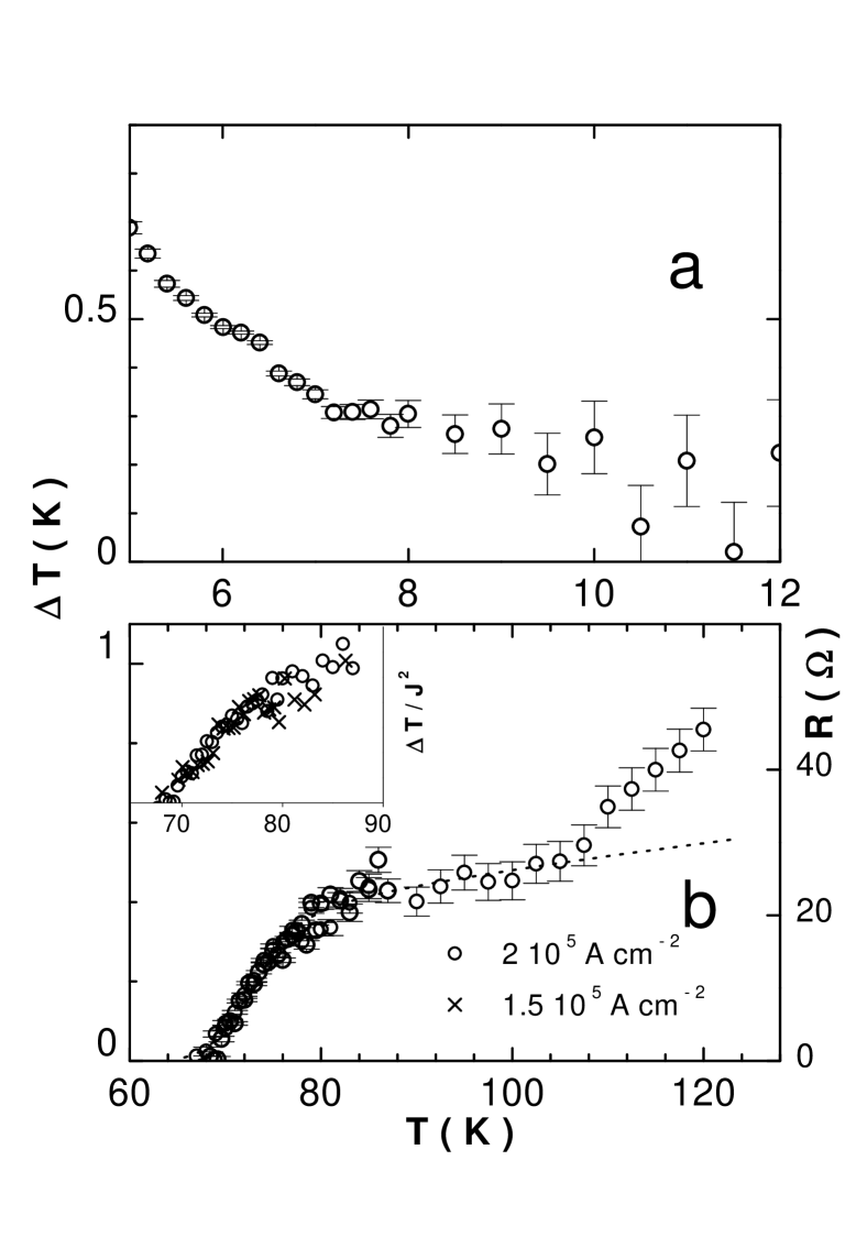
Figure 1: Sample Ia (a) and sample II (b): temperature difference between the sample holder and the film, as measured by the probe pulse.

The temperature increase for the over-doped Bi₂Sr₂CaCu₂O_8+x thin film (sample II) is shown in Fig. 1b. The resistance of the current contacts for this sample was $20\;\Omega$. As can be seen from the comparison with the resistance of the sample and, also, from the scaling of the sample heating with $J^{2}$, the data may be described using the simple evaluation: $(T_{sample}-T_{experiment})\propto R(T_{0},J)\;J^{2}$ below $\sim 100$ K. This demonstrates that the strip temperature is essentially determined by the heating power in the film constriction rather than by the one dissipated in the current contacts. Using the probe value as the actual sample temperature, a slight broadening of the transition remains which must be attributed to the transport current (Fig. 2b).

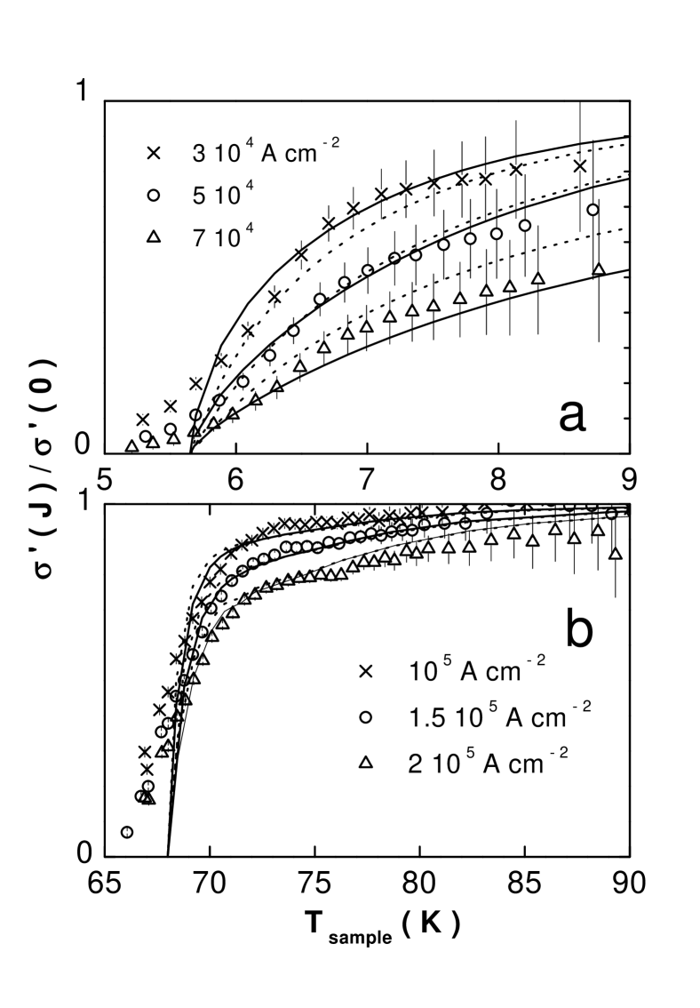
Figure 3: Sample Ia (a) and sample II (b): normalized excess conductivity. Dotted line is Ref. schmidt69 Gaussian approximation using $T_{c}=5.65$ K and $E_{0}=1900$ Vm^-1 for sample Ia and $T_{c}=68$ K and $E_{0}=3\;10^{5}$ Vm^-1 for sample II. Full line is ref. puica03 Eqs.(24),(29) , using respectively $E_{0}(T_{c})=3700$ Vm^-1 and $E_{0}(T_{c})=4.7\;10^{5}$ Vm^-1.

The reduced excess conductivity was obtained as : $\sigma^{\prime}(J)/\sigma^{\prime}(J=0)=R(0)(R_{n}-R(J))/R(J)(R_{n}-R(0))$, where $R_{n}$ is the normal state resistance. $R_{n}$ was obtained from the extrapolation to below $T=130$ K of the empirical function $R=a+b\;T^{\alpha}$ for this overdoped samplekon00 , which fitted the data in the temperature interval 130–300 K with $\alpha=1.13$. As can be seen in Fig. 3, the broadening of the transition corresponds to a drop of the reduced excess conductivity from the normal state asymptotics $\sigma^{\prime}(J)/\sigma^{\prime}(0)=1$ to zero with decreasing temperature. A similar, but far more dramatic, behavior is observed for the Bi₂Sr₂CuO_6+x thin films. Samples Ia and Id were overdoped, with $\alpha=1.08$ and $\alpha=1.10$ respectively. Samples Ib and Ic were underdoped. For these samples, the normal state resistivity was fitted using an activated law. Indeed, as in the case of underdoped YBa₂Cu₃O_6+xtolpygo96 and Bi₂Sr₂CaCu₂O_8+xkon00 , it was found that the resistivity is well described by the activated law $\rho_{0}+b\;\exp(-\Delta/T)$ below $T^{*}$, and by a linear temperature dependence above. $T^{*}\simeq 65$ K and $T^{*}\simeq 85$ K was found respectively for samples Ib and Ic. As in Ref. tolpygo96 , it was found that $\Delta\simeq T^{*}$. For all samples with $n=1$, the sample heating was found to increase with decreasing temperature (Fig. 1a): this is likely due to the decrease of the sample specific heat and of the thermal conductivity at low temperature. For these samples, the resistivity at temperatures well above the mid-point transition is clearly affected by the transport current, which points to the suppression of the excess conductivity by the current. Finally, we stress that the resistivity curves obtained at constant $J$ are not equivalent to the constant $E$ curves usually obtained from theoretical computations, and that the electric field ($E=R\;I\;/L$) must be calculated for each data point in order to compare with the theoretical results.

Before we compare these results with theory, let us examine the experimental artifacts which may affect the results given above. First, the normal state resistivity, as extrapolated from the high temperature values to the superconducting transition, may not be exact. It can be shown that the error made in the reduced excess conductivity is of the order of $(\delta R_{n}/\sigma^{\prime})^{2}$. So, the error which results from the normal state indetermination drops strongly as one enters the superconducting transition, as evidenced by the error bars in Fig. 3. Also, despite very different normal state approximations were used (power law or activated ones), the characteristic field obtained from the excess conductivity was invariably well below the theoretical one. Thus, it is unlikely that the uncertainty on the normal state resistivity value can account for this central result of our measurements. Then, the accuracy of the sample temperature may be questioned. The error made in the computation of the temperature after the main pulse is critical only for sample II. At the middle of the transition for this sample, the broadening at the highest current density is about 0.6 K. This is larger than the temperature increase (0.2 K)obtained from the probe signal and, due to the high sensitivity of the method in the transition region, noticeably larger than the expected error on the sample temperature. Then, the fast temperature relaxation that occurs after the main pulse should be estimated. After correcting the temperature, the sample resistance values above the superconducting transition (say, 14 K and 100 K for sample Ia and II respectively ) where the effect of current reduces to that of heating, agree within a temperature shift of about 0.2 K. While such a temperature difference would yield a sizeable correction of the results for sample II, this is clearly not so for sample with $n=1$. Finally, it may be argued that the sample inhomogeneities affect the transition and its broadening with electric field. The finite width of the transition ( $\simeq 8$ K, $\simeq 2$ K, $\simeq 3$ K, $\simeq 3$ K and $\simeq 5$ K for the 10%–90% transition completion of samples II, Ia, Id, Ib and Ic respectively) could be partly attributed to the inhomogeneities that are present in the sample. While it should be stressed that, a contrario, a narrow transition does not necessarily mean a more homogeneous sample and that intrinsic fluctuations also result in a broadening of the transition (see Fig. 2b), this could be indeed a serious limitation in the present case. As will be seen later, the universal behavior observed for the $n=1$ samples, independently of their oxygen concentration, rules out such an interpretation in this case.

The theoretical results considering only non interacting fluctuations, i.e. Gaussian ones, for a 2D system were given in Refs. hurault69 ; schmidt69 ; tsuzuki69 ; gorkov70 . In this case, the normalized excess conductivity is simply given by :

$$\sigma^{\prime}(T,E)/\sigma^{\prime}(T,0)=\int_{0}^{\infty}dx\exp\{-x-[E/E_{c}(T)]^{2}x^{3}\}$$ (1)

where $E_{c}(T)=E_{0}\;\epsilon^{3/2}$, $E_{0}=16\sqrt{3}k_{B}\;T_{c}/\pi\;e\;\xi_{0}$ and $\epsilon=(T-T_{c})/T_{c}$. The Gaussian result is found to account roughly for the data for all samples (Fig. 3). However, the characteristic field obtained from these fits is $E_{0}\simeq 10^{3}$ Vm^-1 for samples with $n=1$ and $E_{0}\simeq 3\;10^{5}$ Vm^-1 for sample II. These values are considerably smaller than the theoretical estimates $E_{0}=10^{6}$ Vm^-1 and $E_{0}=3\;10^{7}$ Vm^-1 (using $\xi_{0}=40$ Å and $\xi_{0}=20$ Årespectively). As shown in Ref. puica03 , there is an enhanced suppression of the excess conductivity, below the zero-field transition temperature, when critical fluctuations are taken into account within the Hartree approximation. Such an enhancement may result in a decrease of the apparent value for $E_{0}$ when only Gaussian fluctuations are considered. Within the Hartree approximation, the magnitude of the fluctuation renormalization is essentially determined by the Ginzburg number and the anisotropy of the superconductivity. These parameters determine the shift of the superconducting transition temperature with respect to the bare mean field temperature and, associated to this shift, there is an enhancement of the superconducting fluctuations. For sample II, using $s=15.35$ Å, $\xi_{0c}=0.2$ Å, $\kappa=100$ for the superconducting plane separation, the transverse coherence length and the Ginzburg Landau parameter respectively, it is found —as a result of the quasi-2D character for this material— that the bare mean field characteristic temperature calculated according Ref. puica03 ; ullah91 is larger by about 30 K than the superconducting transition temperature (in Ref. puica03 the fluctuating modes are cut for $k^{2}>c\;\xi_{0}^{-2}$ and we have used here $c=1$). Such a difference results in a large enhancement of the superconducting fluctuations with respect to the Gaussian approximation. This clearly fails to account for the experimental data taken at $E=0$ (Fig. 2b). Critical fluctuations from the Hartree approximation and the raw superconducting parameters given above are then clearly strongly overestimated in the region of interest for our data, and it is not surprising that we were unable to obtain a satisfying fit of the reduced excess conductivity in this case. However, the Hartree approximation results were used in Ref. livanov97 to provide convincing fits of the resistivity data under a magnetic field. The anisotropy parameter obtained from these fits was $r=(2\xi_{0c}/s)^{2}=5\,10^{-3}$ and the Ginzburg number (using the notation from Ref. puica03 ) was $g=G_{i}^{2}/4T_{c}=4.5\,10^{-5}$ K^-1, while, from the raw superconducting parameters given above, one obtains $r=1.7\,10^{-4}$ and $g=6.7\,10^{-4}$  K^-1. These differences both contribute to a decrease of the magnitude of the superconducting fluctuations, and the prediction for the zero field resistivity using the same parameter values as Ref. livanov97 now agrees more reasonably with the experimental data (Fig. 2b) (although some part of the transition broadening is likely due to the sample inhomogeneity). Following the formalism of Ref. puica03 , the reduced excess conductivity for such $r$ and $g$ values is now essentially that of the Gaussian regime (here, $E<5\,10^{3}$ Vm^-1) and the experimental data may be fitted using $E_{0}(T_{c})=4.7\,10^{5}$ Vm^-1 (Fig. 3b).

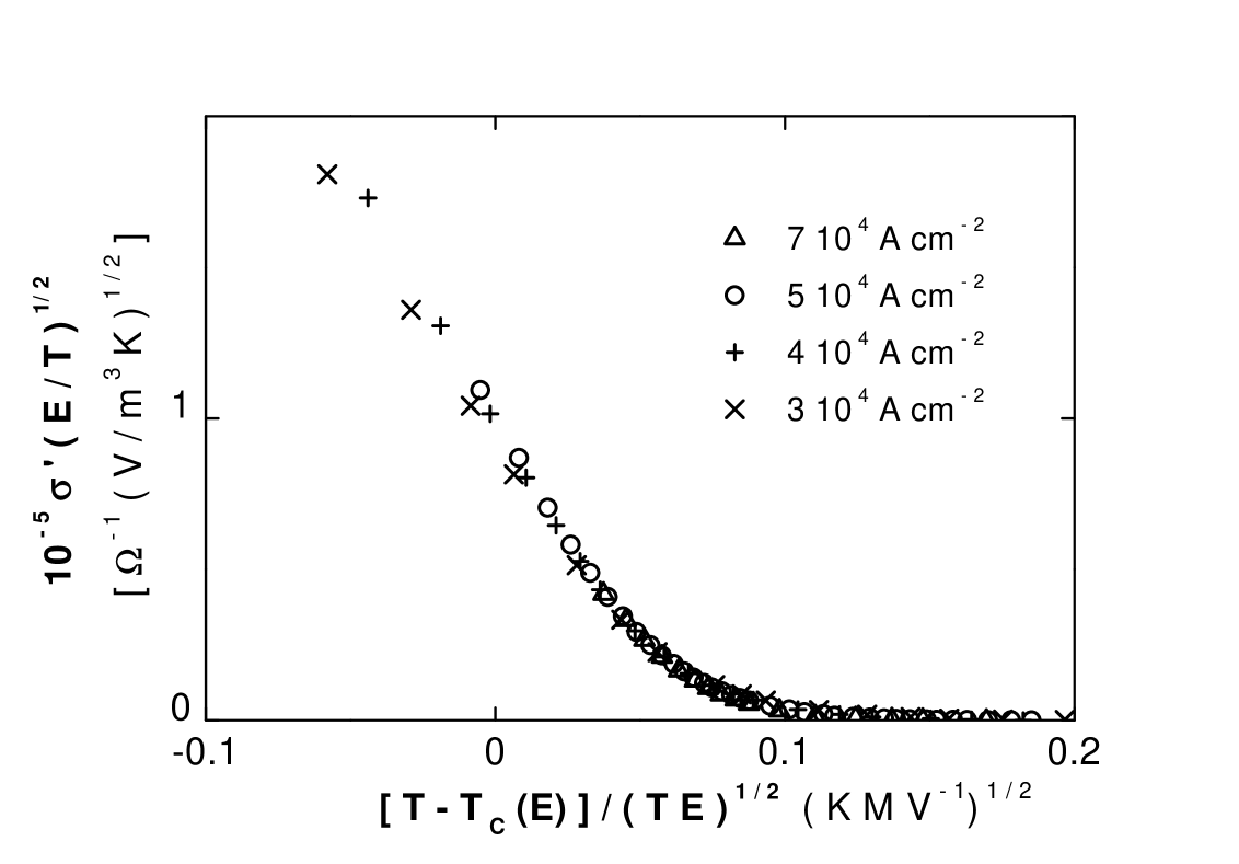
Figure 4: Sample Ia: 2D scaling, using linear $T_{c}(E)$.

In the case of samples with $n=1$, using the following parameters : $s=12.3$ Å, $\xi_{0c}=2$ Å, $\kappa=100$, the bare mean field transition temperature is only shifted by about 0.4 K with respect to the superconducting transition temperature. The critical region should then be much narrower than for sample II and, logically, the Gaussian and the Hartree approximations give close results for $E_{0}$ (Fig. 3a), i.e. well below the above theoretical estimate for all $n=1$ samples (Table 1). The Results of Ref. puica03 should also be valid also for $T<T_{c}$ where the normalized excess conductivity is zero. As pointed out in Ref. puica03 , the treatment of the electric field dependence of the excess conductivity within the Hartree approximation naturally yields results comparable to those obtained in the case of a magnetic field, within the same approximationullah91 . As a result, one may expect that the excess conductivity also scales with temperature and electric field, as was observedwelp91 in the case of a magnetic field. As shown in Fig. 4, the fluctuation conductivity is found to scale according to the two-dimensional law ullah91 : $\sigma^{\prime}\propto(T/E)^{1/2}\mathcal{F}[(T-T_{c}(E))/(T\;E)^{1/2}]$, provided one takes $dT_{c}(E)/dE$ a constant as given in Table 1. A three-dimensional law ($\sigma^{\prime}\propto(T^{2}/E)^{1/3}\mathcal{F}[(T-T_{c}(E))/(T\;E)^{2/3}]$), yields a slightly less satisfying scaling, but comparable $dT_{c}(E)/dE$ value. The critical temperature field dependence obtained in this way confirms the fit of the reduced excess conductivity with the results in ref.puica03 , as the critical field $T_{c0}(dT_{c}/dE)^{-1}$ is also well below the theoretical estimate (Table  1).

Thus, there are converging experimental pieces of evidence that the apparent characteristic field —at least for samples with $n=1$, for which the transition broadening is much larger than the error possibly made for the sample temperature— is well below the one expected from a simple estimate of the depairing field. Several explanations may be considered for this. First, it is known that the existence of ’hot spots’, where the sample temperature locally exceeds $T_{c}$, may drive the sample into the normal state. Such instabilities must be ruled out above $T_{c}$, i.e. in the analysis of the reduced conductivity. Below $T_{c}$, the characteristic current density for which hot spots develop may be estimated to be skocpol74 $10^{10}\;(T_{c}-T)^{1/2}$ Am^-2, well above current densities which significantly affect the resistive curve of $n=1$ samples. Then, as noticed above, the transition width of the sample is finite, which may be interpreted as the result of a distribution of the superconducting temperature. The effect of $T_{c}$ inhomogeneities on the superconducting transition is complicated and the full percolation problem (with a non-linear conductivity) should be considered in the general case. The situation is more simple when the resistivity is close to the normal state value, as the assumption of a uniform current density may be used. Using this assumption in the case of the larger current displayed in Fig. 2a and the results of Ref. puica03 , it is found that the resistivity curve for a field $E/E_{0}\simeq 10^{-4}$, as would be expected from the theoretical estimates above, is only weakly affected by a distribution of $T_{c}$ with a typical width of 1.5 K. In addition, within the hypothesis that this $T_{c}$ distribution strongly influences the apparent value for the characteristic electric field, one would expect that this parameter would be highly sensitive to the oxygen doping state. This is clearly not so, as demonstrated in the case of the $n=1$ samples (Table 1): although the optimal doping might coincide with a maximum in $E_{0}$, the characteristic electric field is well below the depairing estimate for all samples. Another possible explanation for the apparent weakness of the critical field is that the observed current-induced resistivity is the one of the intergranular material. Such a contribution is unlikely for these epitaxial films where grains (typically 0.1 $\mu$m large) are well oriented by the substrate and exhibit sharp (0^∘–90^∘) grain boundaries at the atomic level. It is known also that granular bulk or thin films materials close to $T_{c}$ are invariably in the Ginzburg-Landau regime, where the critical current is the one needed for the suppression of the order parameter in the grainsdarhmaoui96 . Moreover, this would require that the intergranular weak links contribution to the resistivity is comparable to the normal state value, which would likely imply a two step transition curve (corresponding to the Ginzburg-Landau to the Ambegaokar-Baratoff behavior crossover temperature) at large currents, which is not observed here. The scaling of the data according to the prediction of the depairing mechanism rather suggests that a microscopic mechanism (at the coherence length scale) should be found. Microdomains at this scale or belowpan01 is one of such candidates and it has already been noticed that they may affect the magnitude of the depairing currentdarhmaoui96 . Along this line, it is worth mentioning that the $n=1$ material also exhibits a peculiar behavior with respect to the superconducting Nernst effect. Indeed, whereas the Nernst effect for YBa₂Cu₃O_6+x and Bi₂Sr₂CaCu₂O_8+x shows a peak which shifts with magnetic field to lower temperature in a way similar to the resistive transitionri94 , the underdoped $n=1$ material has shown a nearly field independent peakcapan03 . Moreover, the Nernst effect clearly has its maximum well above the resistive transition temperature (i.e. in the fluctuation regime), whereas this peak points —at zero field— towards the completed resistive transition in the case of the two former compounds. As underlined in Ref. capan03 , this discrepancy between the resistive and the Nernst effect transitions may be due to an anomalously large vortex contribution, such as the one arising from a vanishing vortex viscosity. Such a mechanism could account for an enhanced dissipation with current, as observed here. The existence of a phase coherence length distinct from the amplitude one, as proposed in the case of microscopic inhomogeneitypan01 , may also account for these anomalies. Finally, the contribution of the $d$-wave symmetry to the depairing field should also be considered as, in the nodal directions, the depairing field is virtually zero: although there is to our knowledge no theoretical evaluation in this case, we expect a decrease of the critical field with respect to the conventional $s$-wave symmetry, as well as an in-plane angular dependence of the non-linear resistivity. Clearly, further studies of the effect of large electric field, in particular on compounds which have shown distinct resistive and thermodynamic lines —such as Tl₂Ba₂CuO_6+δcarrington96 — are needed to clarify these mechanisms.

Table 1: Sample parameters

Sample	n	$T_{c}(K)$	doping	$E_{0}$	$T_{c}(dT_{c}/dE)^{-1}$
		(K)		$Vm^{-1}$	$Vm^{-1}$
II	2	67.4	overdoped	$4.7\;10^{5}$	-
Ia	1	5.65	overdoped	$3.7\;10^{3}$	$9.5\;10^{2}$
Ib	1	9.8	underdoped	$7.8\;10^{3}$	$1.5\;10^{3}$
Ic	1	14.4	underdoped	$1.5\;10^{4}$	$4.8\;10^{3}$
Id	1	5.1	overdoped	$1.8\;10^{3}$	$3.8\;10^{2}$

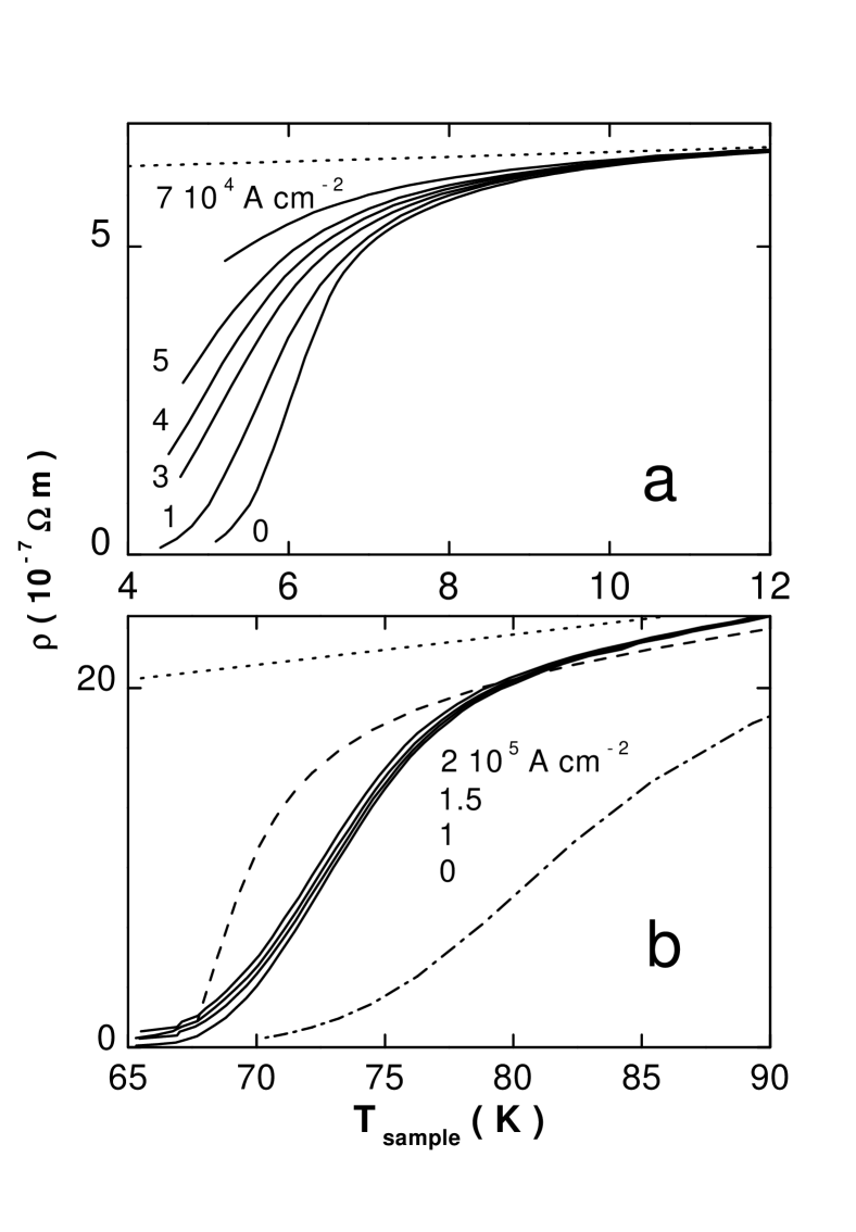
Figure 2: Sample Ia (a) and sample II (b): resistivity vs sample temperature. Dotted line: the extrapolated normal state resistivity $a+bT^{\alpha}$; dashed line: Hartree approximation using the parameters in Ref. livanov97 ; dashed dotted line: Hartree approximation using the raw superconducting parameters.