Quasiclassical theory of charge transport in disordered interacting electron systems

Abstract.

We consider the corrections to the Boltzmann theory of electrical transport arising from the Coulomb interaction in disordered conductors. In this article the theory is formulated in terms of quasiclassical Green’s functions. We demonstrate that the formalism is equivalent to the conventional diagrammatic technique by deriving the well-known Altshuler-Aronov corrections to the conductivity. Compared to the conventional approach, the quasiclassical theory has the advantage of being closer to the Boltzmann theory, and also allows description of interaction effects in the transport across interfaces, as well as non-equilibrium phenomena in the same theoretical framework. As an example, by applying the Zaitsev boundary conditions which were originally developed for superconductors, we obtain the $P(E)$-theory of the Coulomb blockade in tunnel junctions. Furthermore we summarize recent results obtained for the non-equilibrium transport in thin films, wires and fully coherent conductors.

1. Introduction

More than a hundred years ago Drude put forth a theory of metallic conduction [1, 2]. In his theory electrons are treated as a gas of particles which are assumed to move along classical trajectories until they collide with one another or with the ions. The collisions abruptly alter the velocity of the electrons, as illustrated in Fig. 1. Since that time several details of Drude’s theory have been improved. In Drude’s time, for example, it seemed reasonable to assume that the electronic velocity distribution at equilibrium was given by the Maxwell-Boltzmann distribution. About a quarter of a century later, Sommerfeld replaced the Maxwell-Boltzmann distribution by the Fermi-Dirac distribution. A further important step was the description of collisions beyond the relaxation time approximation, which finally led to the Boltzmann equation for the dynamics of the distribution function. In many cases the transport theory based on the Boltzmann equation successfully describes the electrical conductivity of metals. On the other hand the Boltzmann theory still assumes that electrons move along classical trajectories, and quantum mechanical interference effects are neglected. The latter become important at a high concentration of defects or in very small systems. Therefore, in the limits of strong disorder or small system size, the Boltzmann equation fails and the transport becomes non-classical.

Alternatively, following Landauer [3], one can adopt a quantum mechanical description of charge transport: Consider, for example, a constriction as shown in Fig. 2. An incoming electron wave is transmitted or reflected at the constriction with amplitudes $t$ and $r$. The current is then proportional to the transmission probability, i.e. the squared modulus of the amplitude. For simplicity, we restrict ourselves to zero temperature and a one-dimensional conducting channel for now. By assuming two different chemical potentials in the left and right reservoir, $\mu_{L}=\mu_{R}+eV$, the current through the constriction is given by

$$I=2e\int_{\mu_{R}}^{\mu_{L}}\!\!{\rm d}\epsilon\,{\cal N}(\epsilon)v(\epsilon)|t|^{2};$$ (1)

the factor two is due to the electron spin. The product of the density of states ${\cal N}(\epsilon)$ times the velocity $v(\epsilon)$ does not depend on energy and is equal to ${\cal N}v=1/2\pi\hbar$. As a result the conductance of the constriction is determined as

$$G=2\frac{e^{2}}{h}|t|^{2},$$ (2)

with $h/e^{2}\approx 25.8\,{\rm k\Omega}$.

Figure 1. The classical picture for charge transport in metals: electrons move through the metal along classical trajectories. From time to time they scatter and transfer momentum to the lattice.

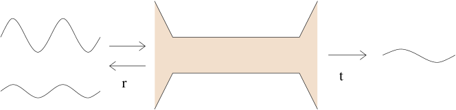
Figure 2. The quantum mechanical picture for electron transport: an incoming electron wave is transmitted or reflected.

The connection between the scattering amplitudes and the conductance was first proposed by Landauer [3]. Generalizations of the conductance formula (2), including for example many transport channels and more than two leads, have been discussed intensively in the literature [4, 5, 6, 7, 8, 9]. The Landauer approach to the conductance has been successfully applied to describe transport through structures where the quantum mechanical coherence of the electron wave functions is maintained over the full system. A fascinating example is the transport through quantum point contacts, which has been studied using both, semiconductor devices [10, 11] as well as single atoms [12].

In the following, we will focus on the transport in metallic systems, where the classical approach to the conductivity is still a good starting point, but quantum effects give rise to various types of corrections to the Drude conductivity. The two corrections that will be considered in this review are weak localization, which is a pure one-particle phenomenon, and effects arising from the combination of disorder and electron-electron interactions.

In order to give a simple idea of how these quantum corrections arise and to highlight the connection between the semiclassical and Landauer’s approach, we present here a physical picture of the origin of weak localization. For reviews on this subject see [13, 14, 15, 16, 17, 18]. The weak localization correction to the conductivity arises as a result of the quantum interference of electron waves in disordered systems.

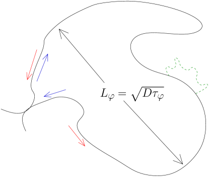
Figure 3. A self-intersecting path as it is relevant for the weak localization correction to the conductivity. The dashed wavy line represents an inelastic scattering event which is responsible for phase breaking; $\tau_{\varphi}$ is the phase coherence time, and $D$ is the diffusion constant.

To travel from point $A$ to point $B$ electrons move along classical paths. In order to obtain the total probability for a transfer from point $A$ to $B$, in classical physics, one has to sum the probabilities for a particle to move along all possible paths. In quantum mechanics one has to sum the amplitudes of each path and take the modulus squared at the end. The relevant paths for weak localization are those with self-intersections and with the velocities of the incoming and outgoing paths in opposite directions as shown in Fig. 3. An electron can travel around the path clockwise or anti-clockwise. The two paths can be assigned an amplitude $\Psi_{1}$ and $\Psi_{2}$; the probability is then proportional to

$$|\Psi_{1}+\Psi_{2}|^{2}=|\Psi_{1}|^{2}+|\Psi_{2}|^{2}+2{\rm Re}(\Psi_{1}^{*}\Psi_{2}).$$ (3)

The first two terms on the right hand side correspond to the classical probabilities. The third term, giving the interference between $\Psi_{1}$ and $\Psi_{2}$, only appears in quantum mechanics. For the special type of paths considered, the interference term is always positive, i.e. due to interference the probability of the process is enhanced. Neglecting the interference corresponds to a classical description of the electrons (Drude-Sommerfeld theory, Boltzmann equation).

This article summarizes recent contributions to the theoretical description of transport in mesoscopic conductors. The central questions addressed are the following:

• In which way is transport modified by electron-electron interactions?

• What happens in the presence of a large voltage, when linear response theory fails?

Both questions are relevant for the interpretation of experiments: Shortly after the discovery of weak localization, it was found that similar effects in the conductivity are caused by the electron-electron interaction [19, 20, 21, 22]. Furthermore electron-electron interactions are also relevant for weak localization itself, since they provide a mechanism for phase breaking. However, while it is clear that inelastic scattering contributes to dephasing, the exact way this happens is far less obvious, as is evident from the recent debates in the literature [23, 24, 25, 26, 27, 28, 29, 30]. The importance of studying non-linear transport is also apparent: Several transport experiments on mesoscopic samples are carried out at low temperatures. Under these conditions inelastic scattering events which drive the electron system towards local equilibrium freeze out. Therefore non-equilibrium conditions can be realized even at rather low voltages.

Here we will use the quasiclassical formalism which, as its historical predecessor, i.e. the Boltzmann equation, is very powerful in dealing with situations far from thermal equilibrium. This was, for example, exploited in studying the dynamics of superconductors in the 1960s and 1970s [31] and hybrid mesoscopic systems in the 1990s [32]. In particular, we will show, that the quasiclassical method provides a convenient framework to describe both quantum interference (weak localization) and Coulomb interaction effects in normal-conducting systems out of equilibrium.

Outline

The article is arranged as follows: In section 2 we introduce the Green’s function technique in the non-equilibrium (Keldysh) formulation, which is the main theoretical tool used throughout this article. In particular, after giving the definition of the quasiclassical Green’s function, we derive the equation of motion as well as the boundary conditions to be used in the presence of interfaces. Following the literature we will demonstrate how a Boltzmann-like theory and the Drude conductivity are recovered within this formalism. In section 3 transport beyond the Drude-Boltzmann theory will be considered. By extending the formalism of section 2 contributions to the current density due to “maximally crossed diagrams” and due to the Coulomb interaction will be calculated.

Sections 4 and 5 will be devoted to applications, i.e., the general expression for the current density of section 3 will be evaluated explicitly for different experimental setups. To begin with, in section 4, we will consider the limit of weak electric field and derive the well-known expression for the Coulomb correction to the Drude conductivity. This will be followed by a discussion of the the non-linear conductivity in films. Furthermore we will investigate the question of whether the phase coherence time $\tau_{\varphi}$, which is a central quantity for weak localization, is relevant for the Coulomb interaction corrections to the conductivity as well. In section 5 we will analyze non-linear transport in wires and in the presence of interfaces. In order to illustrate the power of the method we first show how to obtain the Coulomb blockade theory. We will also discuss the different regimes that arise depending on how the length of the wire compares with the thermal diffusion, inelastic electron-electron and electron-phonon lengths. Chapter 6 summarizes the main results.

A few technical details are provided in the appendices. In appendix A we outline the correspondence of the quasiclassical formalism with the field-theoretic approach based on the non-linear sigma model. In appendix B, we provide the technical details necessary to include the spin degrees of freedom.

2. The classical theory of transport

The traditional transport theory in metals is based on the Boltzmann equation. The central object is the distribution function $f({\bf k},{\bf r},t)$, where $f({\bf k},{\bf r},t){\rm d}{\bf r}\,{\rm d}{\bf k}/(2\pi)^{3}$ is the number of electrons (per spin direction) at time $t$ in the phase space volume ${\rm d}{\bf r}\,{\rm d}{\bf k}$. The charge and current densities are given by

$$\rho({\bf r},t) = (-2e)\int{{\rm d}{\bf k}\over(2\pi)^{3}}f({\bf k},{\bf r},t),$$ (4)

$${\bf j}({\bf r},t) = (-2e)\int{{\rm d}{\bf k}\over(2\pi)^{3}}{\hbar{\bf k}\over m}f({\bf k},{\bf r},t).$$ (5)

In thermal equilibrium the distribution function reduces to the Fermi function. The Boltzmann equation determines the dynamics of the distribution function, and reads

$$\partial_{t}f+{\bf v}\cdot\nabla_{\bf r}f+{1\over\hbar}{\bf F}\cdot\nabla_{\bf k}f=I[f].$$ (6)

The left hand side of the above equation contains information on the energy spectrum, $\hbar{\bf v}=\nabla_{\bf k}\epsilon({\bf k})$, and the external forces ${\bf F}$, whereas the collision term on the right hand side describes the scattering processes. For example, for impurity scattering, the collision term is given by

$$I[f]=-\int{{\rm d}{\bf k}^{\prime}\over(2\pi)^{3}}W_{{\bf k},{\bf k}^{\prime}}[f({\bf k})-f({\bf k}^{\prime})].$$ (7)

In this section we will recall how a Boltzmann-like kinetic equation is derived within the Green’s function formalism. To this end we use the non-equilibrium Green’s function technique, as originally formulated by Keldysh [33]. Our notation will mainly follow [34]. After giving a few general definitions, we will introduce the quasiclassical Green’s function. In the presence of impurity scattering, within the Born approximation for the self-energy, a Boltzmann-like kinetic equation and the Drude formula for the conductivity are recovered. To go beyond the semiclassical treatment and obtain the quantum corrections to the conductivity, to be discussed in sections 3 – 5, further approximations are necessary. From now on we set $\hbar=k_{B}=1$, except in the final results, where, for clarity, we re-introduce the physical constants.

2.1. The Keldysh formalism

An object possessing a simple perturbation expansion is the so-called contour-ordered Green’s function defined by

$$G(x_{1},x_{2})=-{\rm i}\langle T_{c}\Psi(x_{1})\Psi^{\dagger}(x_{2})\rangle,$$ (8)

where $\Psi$ and $\Psi^{\dagger}$ are the usual fermion operators in the Heisenberg picture, and $x_{i}=({\bf x}_{i},t_{i})$. The brackets $\langle\dots\rangle$ denote an average over a statistical ensemble. The times $t_{i}$ vary on a (complex) contour which starts at some time $t_{0}$, and passes once through $t_{1}$ and $t_{2}$ as shown in Fig. 4. The contour-ordering operator $T_{c}$ orders the Fermi operators along the contour.

Figure 4. A closed time path contour, passing through $t_{1}$ and $t_{2}$.

Here we consider a special contour, the “Keldysh contour”. It consists of two parts: The first part starts at $t_{0}=-\infty$ and ends at $t=+\infty$, whereas the second part starts at $+\infty$ and goes back to $-\infty$. The contour-ordered Green’s function on this contour can then be mapped on a two by two matrix in “Keldysh space”,

$$G(x_{1},x_{2})\to\check{G}=\left(\begin{array}[]{cc}G_{11}&G_{12}\\ G_{21}&G_{22}\end{array}\right)$$ (9)

with

$$G_{11}(x_{1},x_{2}) = -{\rm i}\langle T\Psi(x_{1})\Psi^{\dagger}(x_{2})\rangle$$ (10)

$$G_{12}(x_{1},x_{2}) = +{\rm i}\langle\Psi^{\dagger}(x_{2})\Psi(x_{1})\rangle$$ (11)

$$G_{21}(x_{1},x_{2}) = -{\rm i}\langle\Psi(x_{1})\Psi^{\dagger}(x_{2})\rangle$$ (12)

$$G_{22}(x_{1},x_{2}) = -{\rm i}\langle\tilde{T}\Psi(x_{1})\Psi^{\dagger}(x_{2})\rangle;$$ (13)

here $T$ and $\tilde{T}$ are the ordinary time-ordering and anti time-ordering operators. It follows from the definition that the components of $\check{G}$ are not independent, and it is convenient to transform the matrix $\check{G}$ as

$$\check{G}\to{1\over 2}\left(\begin{array}[]{rr}1&-1\\ 1&1\end{array}\right)\left(\begin{array}[]{rr}1&0\\ 0&-1\end{array}\right)\check{G}\left(\begin{array}[]{rr}1&1\\ -1&1\end{array}\right).$$ (14)

In this new representation the Green’s function is

$$\check{G}=\left(\begin{array}[]{cc}G^{R}&G^{K}\\ G^{Z}&G^{A}\end{array}\right),$$ (15)

with

$$G^{R}(x_{1},x_{2}) = -{\rm i}\Theta(t_{1}-t_{2})\langle\Psi(x_{1})\Psi^{\dagger}(x_{2})+\Psi^{\dagger}(x_{2})\Psi(x_{1})\rangle$$ (16)

$$G^{A}(x_{1},x_{2}) = +{\rm i}\Theta(t_{2}-t_{1})\langle\Psi(x_{1})\Psi^{\dagger}(x_{2})+\Psi^{\dagger}(x_{2})\Psi(x_{1})\rangle$$ (17)

$$G^{K}(x_{1},x_{2}) = -{\rm i}\langle\Psi(x_{1})\Psi^{\dagger}(x_{2})-\Psi^{\dagger}(x_{2})\Psi(x_{1})\rangle$$ (18)

$$G^{Z}(x_{1},x_{2}) = 0.$$ (19)

To appreciate the physical meaning of the various Green’s functions, let us consider first non-interacting electrons. The retarded and advanced Green’s functions can then be expressed in terms of the eigenfunctions $\psi_{\lambda}$ and eigenenergies $\epsilon_{\lambda}$ of the single-particle Hamilton operator, so that

$$G^{R(A)}_{\epsilon}({\bf x}_{1},{\bf x}_{2})=\sum_{\lambda}{\psi_{\lambda}({\bf x}_{1})\psi_{\lambda}^{*}({\bf x}_{2})\over\epsilon-\epsilon_{\lambda}\pm{\rm i}0}.$$ (20)

We emphasize that these two components of the matrix Green’s function depend only on the energy spectrum of the system, whereas the Keldysh component of the Green’s function carries the information about the statistical occupation of the states. In thermal equilibrium the Keldysh component may be expressed in terms of the retarded and advanced components as $G^{K}_{\epsilon}=[1-2f(\epsilon)](G^{R}_{\epsilon}-G^{A}_{\epsilon})$, where $f(\epsilon)$ is the Fermi function. Generally, the equation of motion for $G^{K}$ constitutes the quantum-kinetic equation. Approximations to this equation lead to the Boltzmann equation, Boltzmann-like equations, and generalizations.

In order to find such an equation we start with the right-hand and left-hand Dyson equations which read

$$(\check{G}_{0}^{-1}-\check{\Sigma})\check{G}=\delta(x_{1}-x_{2}),\quad\check{G}(\check{G}_{0}^{-1}-\check{\Sigma})=\delta(x_{1}-x_{2}),$$ (21)

where the Green’s functions $\check{G}_{0}$, $\check{G}$, and the self-energy $\check{\Sigma}$ are considered as matrices in space, time, and the Keldysh index. $\check{G}_{0}$ is diagonal in the Keldysh index, the space and time dependence being given by ($e=|e|$)

$$\check{G}_{0}^{-1}(x_{1},x_{2})=\left[{\rm i}\partial_{t_{1}}-{1\over 2m}\left(-{\rm i}\nabla_{{\bf x}_{1}}+e{\bf A}(x_{1})\right)^{2}+e\phi(x_{1})+\mu\right]\delta(x_{1}-x_{2}).$$ (22)

Disorder and interactions are contained in the self-energy. In the Keldysh space the self-energy has the same triangular matrix structure as the Green’s function,

$$\check{\Sigma}=\left(\begin{array}[]{cc}\Sigma^{R}&\Sigma^{K}\\ 0&\Sigma^{A}\end{array}\right).$$ (23)

Relation (23) allows us to express the Keldysh component of the Green’s function as

$$G^{K}=G^{R}\Sigma^{K}G^{A}.$$ (24)

For a graphical representation see Fig. 5.

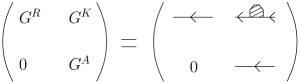
Figure 5. Graphical representation of the Green’s function; we mark $G^{K}$ with a shaded box, which can be understood as the Keldysh component of the self-energy, see Eq. (24).

2.2. The quasiclassical Green’s function

In this subsection we show how to obtain a Boltzmann-like equation. We start by defining the center-of-mass and relative variables

$$\begin{array}[]{ll}{\bf x}={1\over 2}({\bf x}_{1}+{\bf x}_{2}),&{\bf r}={\bf x}_{1}-{\bf x}_{2}\\[2.84544pt] \end{array}$$ (25)

and Fourier transform with respect to the relative coordinate $\bf r$ in order to obtain the Green’s function in the mixed representation

$$G({\bf x}_{1},{\bf x}_{2})\to G({\bf p},{\bf x})=\int{\rm d}{\bf r}{\rm e}^{-{\rm i}{\bf p}\cdot{\bf r}}G({\bf x}+{\bf r}/2,{\bf x}-{\bf r}/2).$$ (26)

In the mixed representation, a matrix product of two objects $A({\bf x}_{1},{\bf x}_{2})$ and $B({\bf x}_{1},{\bf x}_{2})$, as it appears for example in the Dyson equation, becomes [35]

$$(AB)({\bf p},{\bf x})={\rm e}^{-{\rm i}(\partial^{A}_{\bf x}\partial^{B}_{\bf p}-\partial^{A}_{\bf p}\partial^{B}_{\bf x})/2}A({\bf p},{\bf x})B({\bf p},{\bf x}).$$ (27)

When both $A$ and $B$ are slowly varying in $\bf x$ a gradient expansion is justified, i.e. the exponential in the equation above is expanded and only the first term or first few terms are kept.

By subtracting the right-hand from the left-hand Dyson equation and performing a gradient expansion, we obtain the equation of motion for the Green’s function as

$$\left[{\rm i}\tilde{\partial}_{t}+{\rm i}{1\over m}{\bf p}\cdot\tilde{\partial}_{\bf x}\right]\check{G}({\bf p},{\bf x})=\left[\check{\Sigma}({\bf p},{\bf x}),\check{G}({\bf p},{\bf x})\right].$$ (28)

Here the scalar potential $\phi$ and vector potential ${\bf A}$ are included in the gauge invariant derivatives,

$$\tilde{\partial}_{t}\check{G} = \left[\partial_{t_{1}}+\partial_{t_{2}}-{\rm i}e\phi(t_{1})+{\rm i}e\phi(t_{2})\right]\check{G}_{t_{1},t_{2}}({\bf p},{\bf x})$$ (29)

$$= \left[\partial_{t}-{\rm i}e\phi(t+\eta/2)+{\rm i}e\phi(t-\eta/2)\right]\check{G}({\bf p},\eta;{\bf x},t),$$ (30)

and

$$\tilde{\partial}_{\bf x}\check{G}=\left[\partial_{\bf x}+{\rm i}e{\bf A}(t_{1})-{\rm i}e{\bf A}(t_{2})\right]\check{G}_{t_{1}t_{2}}({\bf p},{\bf x}).$$ (31)

In the equation above, $t$ and $\eta$ are center-of-mass and the relative time, defined by

$$t={1\over 2}(t_{1}+t_{2}),\quad\eta=t_{1}-t_{2}.$$ (32)

We introduce next the $\xi$-integrated (quasiclassical) Green’s function

$$\check{g}_{{t_{1}}{t_{2}}}({\hat{\bf p}},{\bf x}) = {{\rm i}\over\pi}\int{\rm d}\xi{\rm d}{\bf r}{\rm e}^{-{\rm i}{\bf p}\cdot{\bf r}}\check{G}\left({\bf x}+{{\bf r}\over 2},t_{1};{\bf x}-{{\bf r}\over 2},t_{2}\right)$$ (33)

$$= \check{g}({\hat{\bf p}},\eta;{\bf x},t),$$ (34)

where $\xi={\bf p}^{2}/2m-\mu$, and ${\hat{\bf p}}$ is a unit vector along the momentum. The $\xi$-integration is understood as a principal value integration, which implies that occasionally suitable (equilibrium) quantities have to be subtracted, in order to ensure convergence. In the entire article we will keep the notation of small $\check{g}$ for the $\xi$-integrated Green’s functions, and capital $\check{G}$ for the original Green’s functions. When approximating the density of states as an energy independent constant, the $\xi$-integration is related to the original integration over the momentum ${\bf p}$ according to

$$\int{{\rm d}{\bf p}\over(2\pi)^{3}}\to{N}_{0}\int{\rm d}\xi\int{{\rm d}\hat{\bf p}\over 4\pi}.$$ (35)

Neglecting the $\xi$-dependence of the self-energy $\Sigma$, and integrating (28) leads to the equation of motion for the quasiclassical Green’s function (Eilenberger equation [36])

$$\left[\tilde{\partial}_{t}+v_{F}\hat{\bf p}\cdot\tilde{\partial}_{\bf x}\right]\check{g}(\hat{\bf p},{\bf x})=-{\rm i}\left[\check{\Sigma}(\hat{\bf p},{\bf x}),\check{g}(\hat{\bf p},{\bf x})\right].$$ (36)

We note that the non-homogeneous term appearing on the right-hand side of the Dyson equation has canceled when deriving the equation of motion for the quasiclassical Green’s function. As a consequence, the latter is determined only by a multiplicative constant. Therefore the equation of motion has to be supplemented by a normalization condition for the Green’s function, which turns out to be of the form “$\check{g}^{2}=1$”, i.e.

$$\int{\rm d}t_{1}\check{g}_{tt_{1}}(\hat{\bf p},{\bf x})\check{g}_{t_{1}t^{\prime}}(\hat{\bf p},{\bf x})=\delta(t-t^{\prime})\check{1},$$ (37)

where $\check{1}$ denotes the unit matrix in the Keldysh space [36, 37]. We now give some relations that are specific for impurity scattering, when it is treated within the self-consistent Born approximation. By assuming a Gaussian, $\delta$-correlated impurity potential one observes that the impurity self-energy is related to the $s$-wave part of the quasiclassical Green’s function,

$$\check{\Sigma}_{t_{1}t_{2}}(\hat{\bf p},{\bf x})=-{{\rm i}\over 2\tau}\int{{\rm d}\hat{\bf p}\over 4\pi}\check{g}_{t_{1}t_{2}}({\hat{\bf p}},{\bf x}),$$ (38)

where $\tau$ is the usual scattering time. Due to the matrix structure of the theory, the above equation is satisfied by all three components (retarded, advanced, Keldysh) of the self-energy. The retarded and advanced self-energies have a simple structure, $\Sigma^{R(A)}_{t_{1}t_{2}}=\mp({{\rm i}/2\tau})\delta(t_{1}-t_{2})$, and the retarded and advanced Green’s functions are given by

$$g^{R(A)}_{t_{1}t_{2}}(\hat{\bf p},{\bf x})=\pm\delta(t_{1}-t_{2}).$$ (39)

We already mentioned that the equation of motion for the Keldysh component of the Green’s function constitutes the kinetic equation. By also transforming to the mixed representation for the frequency/time variables the kinetic equation reads in the present case

$$\left[\tilde{\partial}_{t}+v_{F}{\hat{\bf p}}\cdot\tilde{\partial}_{\bf x}\right]g^{K}({\hat{\bf p}},\epsilon;{\bf x},t)=-\frac{1}{\tau}\left[g^{K}({\hat{\bf p}},\epsilon;{\bf x},t)-\int{{\rm d}{\hat{\bf p}}\over 4\pi}g^{K}({\hat{\bf p}},\epsilon;{\bf x},t)\right],$$ (40)

which clearly reminds us of the Boltzmann equation. A direct connection with the Boltzmann equation has been suggested in [38]. By defining the distribution function as

$$f({\bf p},{\bf x},t)={1\over 2}\left[1-{1\over 2}g^{K}({\hat{\bf p}},\epsilon;{\bf x},t)|_{\epsilon=\xi-e\phi}\right],$$ (41)

and ignoring the explicit dependence of $g^{K}$ on $\hat{\bf p}$ so that the derivatives of $f$ are approximately given by

$$\nabla_{\bf p}f = -{1\over 4}\nabla_{\bf p}\xi\partial_{\epsilon}g^{K}$$ (42)

$$\nabla_{\bf x}f = -{1\over 4}[\nabla_{\bf x}g^{K}-e(\nabla_{\bf x}\phi)\partial_{\epsilon}g^{K}]$$ (43)

$$\partial_{t}f = -{1\over 4}[\partial_{t}g^{K}-e(\partial_{t}\phi)\partial_{\epsilon}g^{K}],$$ (44)

one recovers from the kinetic equation (40) the Boltzmann equation (6) with the external force given by ${\bf F}=e(\nabla_{\bf x}\phi+\partial_{t}{\bf A})$.

Besides the kinetic equation we also need a rule to calculate the physical observables. Generally, the charge and current densities are related to a combination of all components of the Green’s function,

$$\rho({\bf x},t)\! = \!{\rm i}e\left[G^{K}({\bf x},t;{\bf x},t)-G^{R}({\bf x},t;{\bf x},t)+G^{A}({\bf x},t;{\bf x},t)\right]$$ (45)

$${\bf j}({\bf x},t)\! = \!{e\over{2m}}\left[\nabla_{\bf x}\!-\!\nabla_{\bf x^{\prime}}\!+\!2{\rm i}e{\bf A}({\bf x},t)\right]\left[G^{K}-G^{R}+G^{A}\right]({\bf x},t;{\bf x^{\prime}},t)|_{{\bf x^{\prime}}={\bf x}}.$$ (46)

In terms of the quasiclassical Green’s functions, the charge and current densities are [34]

$$\rho({\bf x},t) = 2e{N}_{0}\left[{\pi\over 2}\int{{\rm d}\epsilon\over 2\pi}\int{{\rm d}\hat{\bf p}\over 4\pi}g^{K}(\hat{\bf p},\epsilon;{\bf x},t)-e\phi({\bf x},t)\right]$$ (47)

$${\bf j}({\bf x},t) = e\pi{N}_{0}\int{{\rm d}\epsilon\over 2\pi}\int{{\rm d}\hat{\bf p}\over 4\pi}v_{F}\hat{\bf p}g^{K}({\hat{\bf p}},\epsilon;{\bf x},t).$$ (48)

2.3. Diffusive limit

In this paper we will focus our discussion on the diffusive regime, characterized by small external frequencies and momenta such that $\omega\tau,qv_{F}\tau\ll 1$. Under these conditions the Green’s function becomes almost isotropic and may be expanded in spherical harmonics. In the present case, it is sufficient to retain the $s$- and $p$-wave components,

$$\check{g}(\hat{\bf p},{\bf x})=\check{g}_{s}({\bf x})+\hat{\bf p}\cdot\check{\bf g}_{p}({\bf x}).$$ (49)

By inserting Eq. (49) into the kinetic equation and separating the $s$- and $p$-wave parts, one obtains the relation

$$\check{\bf g}_{p}({\bf x})=-v_{F}\tau\tilde{\partial}_{\bf x}\check{g}_{s}({\bf x}),$$ (50)

and finally the kinetic equation for the $s$-wave component of the Green’s function

$$\left(\tilde{\partial}_{t}-D\tilde{\partial}_{\bf x}\tilde{\partial}_{\bf x}\right)g^{K}_{s}(\epsilon;{\bf x},t)=0,$$ (51)

where we have introduced the diffusion constant $D=v_{F}^{2}\tau/3$. From Eqs. (47) – (50), an explicit expression for the current density follows:

$${\bf j}({\bf x},t)=-e\pi D{N}_{0}\tilde{\partial}_{\bf x}\int{{\rm d}\epsilon\over 2\pi}g^{K}_{s}(\epsilon;{\bf x},t)=-D\nabla_{\bf x}\rho({\bf x},t)+2e^{2}D{N}_{0}{\bf E}({\bf x},t),$$ (52)

in agreement with the Drude formula for the conductivity.

2.4. Boundary conditions

In particular, we will be interested in the transport properties of finite systems, i.e. metallic systems with boundaries to insulators and reservoirs. We note that, due to the $\xi$-integration and the gradient expansion, the quasiclassical equations are not directly applicable across sharp interfaces and therefore must be supplemented by boundary conditions. For a surface with specular scattering, and for the non-interacting case we consider at present, the matching conditions read

$$\check{g}(\hat{\bf p};{\bf x}_{-}) = R\check{g}({\tilde{\hat{\bf p}}};{\bf x}_{-})+T\check{g}(\hat{\bf p};{\bf x}_{+}),$$ (53)

$$\check{g}({\tilde{\hat{\bf p}}};{\bf x}_{+}) = R\check{g}(\hat{{\bf p}};{\bf x}_{+})+T\check{g}({\tilde{\hat{\bf p}}};{\bf x}_{-}),$$ (54)

where $T$ and $R$ are the transmission and reflection probabilities at the surface.

Figure 6. An interface with specular scattering. An incoming particle moving in direction $\hat{\bf p}$ is reflected with probability $R$ into $\tilde{\hat{\bf p}}$, and transmitted with probability $T$ into $\hat{\bf p}$; $\theta$ is the angle between the trajectory and the normal vector $\hat{\bf n}$ of the interface.

$\hat{\bf p}$ and $\tilde{\hat{\bf p}}$ are the directions for incoming, transmitted, and reflected particles as shown in Fig. 6. From the sum of the two equations and using the relation $R+T=1$ it is found that the antisymmetric combination of $g(\hat{\bf p})$ and $g(\tilde{\hat{\bf p}})$ is continuous at the interface,

$$\check{g}(\hat{\bf p};{\bf x}_{-})-\check{g}({\tilde{\hat{\bf p}}};{\bf x}_{-})=\check{g}(\hat{\bf p};{\bf x}_{+})-\check{g}({\tilde{\hat{\bf p}}};{\bf x}_{+}),$$ (55)

from which one observes that the current normal to the interface is conserved, since

$$\int{{\rm d}\hat{\bf p}\over 4\pi}({\hat{\bf n}}\cdot{\hat{\bf p}})\,\check{g}(\hat{\bf p};{\bf x}_{-})=\int{{\rm d}\hat{\bf p}\over 4\pi}({\hat{\bf n}}\cdot{\hat{\bf p}})\,\check{g}(\hat{\bf p};{\bf x}_{+}).$$ (56)

After subtracting (54) from (53) and making use of the continuity of the antisymmetric combination of the Green’s functions it is seen that the symmetric combination of the Green’s functions jumps at the interface, with the size of the jump determined by

$$\check{g}(\hat{\bf p};{\bf x}_{-})-\check{g}({\tilde{\hat{\bf p}}},{\bf x}_{-})={T\over 2R}\left\{\left[\check{g}(\hat{\bf p};{\bf x}_{-})+\check{g}({\tilde{\hat{\bf p}}},{\bf x}_{-})\right]-\left[\check{g}(\hat{\bf p};{\bf x}_{+})+\check{g}(\tilde{\hat{\bf p}},{\bf x}_{+})\right]\right\}.$$ (57)

The generalization of this boundary condition to the interacting case is given below, compare Eq. (152).

After these general considerations we now focus our attention on the diffusive limit. Equation (57) is valid both for clean and dirty metals. In a dirty metal, however, a matching condition which involves only the angular averaged Green’s function $\check{g}_{s}({\bf x})$ instead of $\check{g}(\hat{\bf p};{\bf x})$ would be desirable. Recall that in the diffusive limit the angular dependence of $\check{g}(\hat{\bf p},{\bf x})$ can be taken into account by keeping only the $s$- and $p$-wave parts. One might then be tempted to expand the Green’ functions in (57) in an $s$-wave and a $p$-wave part, multiply (57) by $\hat{\bf p}$, take the angular average and hence obtain the matching conditions in the diffusive limit in terms of the $s$-wave and $p$-wave components of the Green’s functions. However, the task of finding the matching condition turns out to be not that simple, since close to the interface the angular dependence of the transmission and reflection coefficients may generate higher harmonics in the Green’s functions, and it is not justifiable to terminate the expansion after the first two terms. Only at some distance from the interface will such an expansion hold. The task is thus to derive an effective condition which connects the Green’s functions “far” from the interface, i.e. on distances of the order of the elastic mean free path. By integrating the kinetic equation and making use of (57) it has been shown [39, 40, 41] that this matching condition can be written as

$$-D({\hat{\bf n}}\cdot\tilde{\partial}_{\bf x})g_{s}^{K}({\bf x})=\Gamma\left[g_{s}^{K}({\bf x}_{-})-g_{s}^{K}({\bf x}_{+})\right],$$ (58)

where $\Gamma$ is a function of the angular dependent transmission and reflection amplitudes $R$ and $T$. For a strong barrier ($T/R\ll 1$), $\Gamma$ is given by

$$\Gamma=v_{F}\int_{0}^{1}{\rm d}(\cos\theta)\,\cos\theta\,{T(\cos\theta)\over 2R(\cos\theta)},$$ (59)

while for a weak barrier ($R/T\ll 1$)

$$\Gamma=v_{F}{1\over 9}\left[\int_{0}^{1}{\rm d}(\cos\theta)\,\cos^{3}(\theta){2R\over T}\right]^{-1},$$ (60)

see [41]; for a barrier of arbitrary strength the parameter $\Gamma$ may be obtained from the solution of an integral equation [41].

As a simple application of the matching condition (58) we consider a system consisting of a diffusive wire of length $L$ which is attached to two reservoirs. We study the system in a non-equilibrium situation with an applied voltage $V_{l}-V_{r}=V$, where the subscripts $l$ and $r$ indicate the left and right reservoirs, respectively. The classical resistance of the structure is the sum of the wire resistance and the interface resistances, $R_{\rm tot}=R_{\rm wire}+R_{l}+R_{r}$, and the current is $I=V/R_{\rm tot}$. We will demonstrate now how this result can be reproduced within the quasiclassical formalism.

Within the quasiclassical formalism the current flowing in the wire is given by

$$I_{\rm wire} = -e\pi DN_{0}{\cal A}\int{{\rm d}\epsilon\over 2\pi}\partial_{x}g^{K}_{s}(\epsilon,x),$$ (61)

where ${\cal A}$ the cross section, and $x=0\dots L$ is the position along the wire. The reservoirs are assumed to be in thermal equilibrium, with the distribution function given by $g^{K,l,r}_{s}(\epsilon)=2\tanh\left[(\epsilon+|e|V_{l,r})/2T\right]$. The boundary conditions read

$$-D\partial_{x}g^{K}_{s}(\epsilon,x)|_{x=0} = \Gamma_{l}[g^{K,l}_{s}(\epsilon)-g^{K}_{s}(\epsilon,0)]$$ (62)

$$-D\partial_{x}g^{K}_{s}(\epsilon,x)|_{x=L} = \Gamma_{r}[g^{K}_{s}(\epsilon,L)-g^{K,r}_{s}(\epsilon)],$$ (63)

where $\Gamma_{l,r}$ are the transparencies of the left and right interface. The current across the interfaces can be written as

$$I_{l} = -{1\over 2}e\Gamma_{l}{\cal A}N_{0}\int{\rm d}\epsilon[g^{K}_{s}(\epsilon,0)-g^{K,l}_{s}(\epsilon)]$$ (64)

$$I_{r} = -{1\over 2}e\Gamma_{r}{\cal A}N_{0}\int{\rm d}\epsilon[g^{K,r}_{s}(\epsilon)-g^{K}_{s}(\epsilon,L)].$$ (65)

Furthermore we assume that the wire is so short that we can neglect inelastic scattering. In this case the kinetic equation for the distribution function inside the wire simply becomes $-D\partial_{x}^{2}g^{K}_{s}=0$. Solving this equation one finally finds the current as $I=V/(R_{l}+R_{\rm wire}+R_{r})$, with

$$R_{r} = 1/(2e^{2}{\cal A}N_{0}\Gamma_{l})$$ (66)

$$R_{\rm wire} = L/(2e^{2}{\cal A}N_{0}D)$$ (67)

$$R_{l} = 1/(2e^{2}{\cal A}N_{0}\Gamma_{r})$$ (68)

as one would expect for three resistors in series.

3. Quantum interference in diffusive conductors – general formalism

Quantum effects give rise to deviations from the classical expression of the electrical conductivity of a metal: The conductivity depends on the sample specific realization of the impurity potential, and even after averaging over all possible realizations of the impurity potential corrections to the conductivity remain. The quantum corrections to the average conductivity in a metal with diffusive electron motion are weak localization, and the interaction contributions to the conductivity. The latter are often classified as the particle-particle (Cooper) channel, which is related to the exchange of superconducting fluctuations, and the particle-hole channel, which is related to the exchange of charge fluctuations (spin singlet channel) or spin fluctuations (spin triplet channel). In this article we concentrate on the average conductivity, and in particular on the Coulomb interaction in the particle-hole channel. We will neglect the Cooper channel. This is justified in non-superconducting metals, since in this situation the relevant interaction parameter scales down under the renormalization group flow. For completeness we will also discuss briefly weak localization. In this section we will give the general expressions for the contribution to the current density due to weak localization and due to the electron-electron interaction. The following sections 4 and 5 will contain specific applications.

3.1. Weak localization

In a weakly disordered metal, quantum interference leads at low temperature to deviations from the Drude-Boltzmann theory. Gorkov et al. [42] and Abrahams et al. [43] showed that the summation of maximally crossed diagrams gives rise to divergences in the conductivity for arbitrarily weak disorder in dimensions less than and equal to two. This so-called weak localization correction to the conductivity is due to electrons diffusing along closed paths, where quantum interference causes an enhanced backscattering probability, as discussed in the introduction. The weak localization contribution to the current density is given by

$$\delta{\bf j}_{\rm WL}(t)=-e^{2}D{4\over\pi}\int_{\tau}^{\infty}{\rm d}\eta\,C^{t-\eta/2}_{\eta,-\eta}({\bf x},{\bf x}){\bf E}(t-\eta),$$ (69)

where $D$ is the diffusion constant, the short time cut-off $\tau$ in the $\eta$-integration is the elastic scattering time, and $C^{t}_{\eta,-\eta}({\bf x},{\bf x})$ is the cooperon at two coinciding points in space. In the presence of a vector potential, the cooperon is given by the solution of the differential equation

$$\left\{2{\partial\over\partial\eta}-D(\nabla_{\bf x}+{\rm i}e{\bf A}_{C})^{2}\right\}C^{t}_{\eta,\eta^{\prime}}({\bf x},{\bf x}^{\prime})$$

$$=\delta({\bf x}-{\bf x}^{\prime})\delta(\eta-\eta^{\prime}),$$ (70)

with ${\bf A}_{C}={\bf A}({\bf x},t+\eta/2)+{\bf A}({\bf x},t-\eta/2)$. We recall now the results for the conductivity. In the absence of external fields the cooperon at two coinciding points in space is given by

$$C^{t}_{\eta,-\eta}({\bf x},{\bf x})={1\over 2}\left({1\over 4\pi D\eta}\right)^{d/2}{\rm e}^{-\eta/\tau_{\varphi}},$$ (71)

where $d$ is the spatial dimension and a phenomenological dephasing time $\tau_{\varphi}$ has been introduced; microscopically dephasing arises from inelastic scattering. Inserting the above into Eq. (69), one arrives at the standard result [13, 14, 15, 16]

$$\delta\sigma_{\rm WL}=\left\{\begin{array}[]{ll}-{e^{2}\over\pi\hbar}\sqrt{D\tau_{\varphi}}&(d=1)\\[4.30554pt] -{e^{2}\over 2\pi^{2}\hbar}\ln(\tau_{\varphi}/\tau)&(d=2)\\[4.30554pt] {e^{2}\over 2\pi^{2}\hbar}\sqrt{1/D\tau_{\varphi}}+{\rm const}&(d=3).\end{array}\right.$$ (72)

The connection to the Green’s function formalism is the following: In section 2 we demonstrated that, by approximating the impurity self-energy by $\Sigma_{\rm Born}$, the Boltzmann equation for the distribution function and the Drude conductivity are recovered. The kinetic equation including the weak localization correction has been derived in [44], considering also the maximally crossed diagrams,

$$\check{\Sigma}=\check{\Sigma}_{\rm Born}+\check{\Sigma}_{\rm mc},$$ (73)

with

(74)

(75)

The self-energy has to be determined self-consistently. The contributions of the crossed diagrams to the retarded and the advanced self-energies are small and are therefore neglected [45]. The contribution to $\Sigma^{K}_{\rm mc}$ from the diagram with $m$ impurity lines contains the sum of products with ($2m-1$) Green’s functions, $\sum_{n=0}^{2m-2}(G^{R})^{n}G^{K}(G^{A})^{2m-2-n}$, i.e. integrals involving all combinations of the Green’s function from $G^{K}G^{A}\dots G^{A}$ to $G^{R}\dots G^{R}G^{K}$. The momentum integrals reduce to integrals over pairs of Green’s functions of the form

$$\eta^{RR}={1\over 2\pi{N}_{0}\tau}\int{{\rm d}{\bf k}\over(2\pi)^{3}}G^{R}({\bf k},\epsilon)G^{R}(-{\bf k}+{\bf q},\epsilon-\omega),$$ (76)

and the analogously defined integrals $\eta^{AA}$ and $\eta^{RA}$. For small ${\bf q}$ the integrals $\eta^{RR}$ and $\eta^{AA}$ are of the order $1/(\epsilon_{F}\tau)$, whereas the integrals $\eta^{RA}$ are of order one,

$$\eta^{RA}\approx 1-\tau[-{\rm i}\omega+Dq^{2}].$$ (77)

Terms involving $\eta^{RR}$ or $\eta^{AA}$ will thus be neglected. Following this rule the graphs contributing to ${\check{\Sigma}}_{\rm mc}$ are shown in Fig. 7.

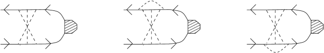
Figure 7. Relevant graphs for the Keldysh component of the self-energy, ${\Sigma}^{K}_{\rm mc}$ (“mc”: maximally crossed). The first graph leads to the term proportional to $g^{K}(-\hat{\bf p})$ in the kinetic equation, the other two graphs are responsible for the term containing an angular average over $g^{K}(\hat{\bf p})$.

In order to understand how the above diagrams modify the kinetic equation, let us examine the first diagram in Fig. 7. In this diagram there is an equal number of retarded and advanced Green’s functions and a Keldysh Green’s function in the middle, i.e., we have a sequence $G^{R}...G^{R}G^{K}G^{A}...G^{A}$. The self-energy of the first diagram of Fig. 7 has the form

$$\delta\Sigma^{K}({\bf p},\epsilon;{\bf q},\omega)={1\over 2\pi N_{0}\tau^{2}}\sum_{{\bf Q}}C({\bf Q},\omega)G^{K}({\bf Q}-{\bf p},{\epsilon};{\bf q},{\omega}),$$ (78)

where Fourier variables ${\bf p},\epsilon$ and ${\bf q},\omega$ refer to relative and center-of-mass coordinates, respectively, and the integration over the cooperon takes care of all the series of maximally crossed diagrams:

$$C({\bf Q},\omega) = \tau\left[\eta^{RA}+(\eta^{RA})^{2}+\dots\right]=\tau\eta^{RA}/[1-\eta^{RA}]$$ (79)

$$\approx {1\over-{\rm i}\omega+DQ^{2}}.$$ (80)

To finally derive the modified Eilenberger equation, the commutator between the self-energy and Green’s function, which appears on the right-hand side of Eq. (28), has to be integrated with respect to $\xi$. As a result we have

$$\frac{1}{\pi}\int{\rm d}\xi\,[{\delta\check{\Sigma}},{\check{G}}]^{K}=\frac{1}{\pi}{1\over 2\pi N_{0}\tau^{2}}\sum_{{\bf Q}}C({\bf Q},\omega)\int{\rm d}\xi G^{K}(G^{R}-G^{A}).$$ (81)

Following [44] we use the Ansatz

$$G^{K}({\bf p},{\bf q})={1\over 2}g^{K}({\hat{\bf p}},{\bf q})\left(G^{R}({\bf p}+{{\bf q}/2})-G^{A}({\bf p}-{{\bf q}/2})\right),$$ (82)

which is based both on the fact that $G^{R}$ and $G^{A}$ are not corrected beyond the Born approximation, and that the equation above gives the correct quasiclassical Green’s function upon $\xi$-integration. A similar analysis can be carried out for the other diagrams of Fig. 7; after some algebra the kinetic equation is found as

$$\left[\tilde{\partial}_{t}+v_{F}\hat{\bf p}\cdot\tilde{\partial}_{\bf x}\right]g^{K}(\hat{\bf p},\eta;{\bf x},t) = -{1\over\tau}\left[g^{K}(\hat{\bf p},\eta;{\bf x},t)-\int{{\rm d}\hat{\bf p}\over 4\pi}g^{K}(\hat{\bf p},\eta;{\bf x},t)\right]$$ (84)

$$+\frac{1}{\tau}\int_{-\infty}^{t}{\rm d}t^{\prime}\alpha(t,t^{\prime})\left[g^{K}(-\hat{\bf p},\eta;{\bf x},t^{\prime})-\int{{\rm d}\hat{\bf p}\over 4\pi}g^{K}(\hat{\bf p},\eta;{\bf x},t^{\prime})\right]$$

$$\alpha(t,t^{\prime}) = {2\over\pi N_{0}}C^{t-\eta^{\prime}/2}_{\eta+\eta^{\prime},\eta-\eta^{\prime}}({\bf x},{\bf x}),\quad\eta^{\prime}=t-t^{\prime},$$ (85)

where we put the general version of the cooperon $C^{t}_{\eta,\eta^{\prime}}({\bf x},{\bf x})$ with three different time arguments as given in (70). The maximally crossed diagrams give rise to an additional scattering term on the right hand side of Eq. (84) which is non-local in time, with the dephasing time as the relevant time scale.

We restrict ourselfes now to the diffusive limit and calculate the change in the current density due to the maximally crossed diagrams. One identifies two contributions. The first term appears because the additional scattering term may change the solution of the kinetic equation for the $s$-wave part of the Green’s function, $g^{K}_{s}\to g^{K}_{s}+\delta g^{K}_{s}$, and

$$\delta{\bf j}_{\rm Born}({\bf x},t) = -e\pi D{\cal N}_{0}\tilde{\partial}_{\bf x}\int{{\rm d}\epsilon\over 2\pi}\delta g^{K}_{s}(\epsilon;{\bf x},t)$$ (86)

$$= -D\nabla_{\bf x}\delta\rho({\bf x},t).$$ (87)

The second term arises from the modified relation between the $s$-wave and $p$-wave contribution to the Green’s function,

$${\bf g}_{p}=-v_{F}\tau\tilde{\partial}_{\bf x}g_{s}+v_{F}\tau\int_{-\infty}^{t}{\rm d}t^{\prime}\alpha(t,t^{\prime})\tilde{\partial}_{\bf x}g_{s}$$ (88)

which leads to

$$\delta{\bf j}_{\rm mc}({\bf x},t) = 2eD\tau\int_{\tau}^{\infty}{\rm d}\eta C^{t-\eta/2}_{\eta,-\eta}({\bf x},{\bf x})\tilde{\partial}_{\bf x}\int{{\rm d}\epsilon\over 2\pi}g^{K}_{s}(\epsilon;{\bf x},t-\eta)$$ (89)

$$= -{2D\over\pi N_{0}}\int_{\tau}^{\infty}{\rm d}\eta C^{t-\eta/2}_{\eta,-\eta}({\bf x},{\bf x})\left[-\nabla_{\bf x}\rho({\bf x},t-\eta)+2e^{2}N_{0}{\bf E}({\bf x},t-\eta)\right].$$ (90)

The total weak localization correction to the current density is thus

$$\delta{\bf j}_{\rm WL}=\delta{\bf j}_{\rm Born}+\delta{\bf j}_{\rm mc}.$$ (91)

In this equation the sum of both terms is needed in order to ensure charge conservation. In the special case where the electric field and the charge density are homogeneous in space, the weak localization correction to the current density, as given in Eq. (69), is recovered.

3.2. Interaction correction to diffusive transport

Shortly after the discovery of weak localization it was found [20, 21, 22] that similar effects in the conductivity are also caused by the electron-electron interaction. The interaction correction to the conductivity in the particle-hole singlet channel, for example, is given by [27]

$$\delta\sigma_{\rm EEI}=-{4e^{2}D\over\pi d}\int_{\tau}^{\infty}{\rm d}\eta\left({\pi T\eta\over\sinh(\pi T\eta)}\right)^{2}\left({1\over 4\pi D\eta}\right)^{d/2}$$ (92)

which leads to

$$\delta\sigma_{\rm EEI}\approx\left\{\begin{array}[]{ll}-4.91{e^{2}\over\pi^{2}\hbar}\sqrt{\hbar D/k_{B}T}&(d=1)\\[4.30554pt] -{e^{2}\over 2\pi^{2}\hbar}\ln(\hbar/k_{B}T\tau)&(d=2)\\[4.30554pt] 1.83{e^{2}\over 6\pi^{2}\hbar}\sqrt{k_{B}T/\hbar D}+{\rm const}.&(d=3)\end{array}\right..$$ (93)

The inclusion of the triplet channels does not change the functional form of the temperature dependence of the correction to the conductivity, but modifies the prefactor, which then depends also on the strength of the electron-electron interaction in the spin triplet channel [46, 47], see also Eq. (124) below.

Whereas a simple and convincing physical interpretation of weak localization exists, we are not aware of as simple an interpretation of the interaction effect. However, attempts have been made [48, 49], and we present the main ideas. First, one observes that the impurities perturb the charge distribution in the metal, $n\to n+\delta n$. For example, a single impurity gives rise to the so-called Friedel oscillations of the density, which persist even at large distance $\delta n(r)\sim\sin(2k_{F}r)/r^{3}$. In the presence of many impurities the electron density becomes non-uniform, with the details depending on the particular distribution of the impurity positions. When both electron interaction and disorder are present, the charge inhomogeneity acts as an additional scattering potential, which, within the Hartree approximation, is given by

$$V_{H}({\bf r})=\int V({\bf r}-{\bf r}^{\prime})\delta n({\bf r}^{\prime}){\rm d}{\bf r}^{\prime}.$$ (94)

It is clear that this additional scattering potential may affect the elastic mean free path. The way this happens, however, is less obvious. In the following we give an argument [48] which shows that the interaction contribution to the conductivity is due to quantum interference. Let us consider two classical paths an electron can follow to travel from point A to point B. Let path “1” and “2” be identical up to an extra closed loop in path “2”, so that there is a phase difference between the two amplitudes, $\Psi_{2}=\exp({\rm i}\varphi_{\rm loop})\Psi_{1}$. The sign of the interference term ${\rm Re}(\Psi_{1}^{*}\Psi_{2})$ is positive or negative, depending on the phase $\varphi_{\rm loop}$, and therefore processes of this type, when averaged over all the impurity configurations, give a negligible small contribution to the total probability for traveling from A to B. This will be different in the presence of electron-electron interactions. To first order in the Hartree potential $V_{H}$ we may write the interference term as ${\rm Re}(\Psi_{1}^{*}\Psi_{2}V_{H})$. Now note that the charge inhomogeneity $\delta n(\bf r)$, and therefore $V_{H}({\bf r})$, is related to (virtual) electrons or holes which propagate along closed paths, since

$$\delta n({\bf r})={{\rm i}\over\pi}\int{\rm d}\epsilon f(\epsilon)\left[G^{R}_{\epsilon}({\bf r},{\bf r})-G^{A}_{\epsilon}({\bf r},{\bf r})\right].$$ (95)

In the case where a virtual hole goes around the same closed loop as the path number “2”, the phase factor $\exp({\rm i}\varphi_{\rm loop})$ cancels, and $\Psi_{1}$ and $\Psi_{2}$ interfere coherently. A graphical representation of the relevant process is shown in Fig. 8.

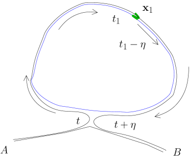
Figure 8. Graphical representation of processes leading to the interaction correction to the conductivity. The figure shows two paths for the propagation from $A$ to $B$. One of the paths contains an extra closed loop. The corresponding phase factor $\exp({\rm i}\varphi_{\rm loop})$ cancels with a phase factor due to a virtual particle which is created at $({\bf x}_{1},t_{1}-\eta)$, propagates along the same closed loop, and is finally absorbed at $({\bf x}_{1},t_{1})$.

The Coulomb correction to the electrical conductivity was investigated in the past with various methods, ranging from standard many-body diagrammatic calculations of the Kubo formula to a field-theoretic description based on a mapping of the original problem of interacting Fermions to a non-linear sigma model for matrix fields, and also to a generalized kinetic equation approach [19, 46, 47, 13, 34, 50, 18, 51, 52, 53]. In the following we will briefly outline how the Coulomb interaction in a disordered medium can be incorporated in the quasiclassical formalism we employ in this article. We start from the kinetic equation and the expression for the current density in the diffusive limit,

$$\tilde{\partial}_{t}\check{g}_{s}-D\tilde{\partial}_{\bf x}(\check{g}_{s}\tilde{\partial}_{\bf x}\check{g}_{s})=0$$ (96)

and

$${\bf j}({\bf x},t)=-e\pi DN_{0}(\check{g}_{s}\tilde{\partial}_{\bf x}\check{g}_{s})^{K}\!({\bf x},t).$$ (97)

These two equations generalize the expressions we gave in section 2 to the situation where the quasiclassical retarded and advanced Green’s functions are not necessarily equal to plus or minus one. The Coulomb interaction is now introduced by adding internal electric fields to the external one,

$$\phi\to\phi^{\rm ext}\check{1}+\check{\phi}^{\rm int},$$ (98)

and physical observables are obtained after averaging over the internal fields. Formally this can be carried out by means of a Hubbard-Stratonovich transformation within a functional integral formalism. More physically, this approach corresponds to describing the Coulomb interaction in terms of the exchange of scalar and longitudinal photons. The internal field has a non-trivial structure in Keldysh space,

$$\check{\phi}^{\rm int}=\left(\begin{array}[]{cc}\phi_{1}&\phi_{2}\\ \phi_{2}&\phi_{1}\end{array}\right),$$ (99)

and the field fluctuations are related to the retarded, advanced and Keldysh components of the (screened) Coulomb interaction,

$$-{\rm i}e^{2}\left(\begin{array}[]{cc}\langle\phi_{1}\phi_{1}\rangle&\langle\phi_{1}\phi_{2}\rangle\\ \langle\phi_{2}\phi_{1}\rangle&\langle\phi_{2}\phi_{2}\rangle\end{array}\right)={1\over 2}\left(\begin{array}[]{cc}V^{K}&V^{R}\\ V^{A}&0\end{array}\right).$$ (100)

In this language, screening effects appear as self-energy corrections of the photon propagators. To stress the difference between an external classical field and an internal quantum one, we observe that $\phi_{1}$ and $\phi_{2}$ are related to the sum and difference of the values that the field takes in the upper and lower parts of the Keldysh contour, respectively. An external field takes the same value on both parts of the Keldysh contour and hence its ($12$)- and ($21$)-components in Keldysh space vanish. Finally we define the distribution function $F$ via the $s$-wave part of the quasiclassical Green’s function according to

$$g^{K}_{s}=g^{R}_{s}F-Fg^{A}_{s}.$$ (101)

We now show how to calculate quantities like the Green’ functions, the density of states or the current density perturbatively in the interaction. For the Green’s function, for example, we write

$$\check{g}([\phi^{\rm int}])=\left(\begin{array}[]{cc}1&2F_{0}\\ 0&-1\end{array}\right)+\left(\begin{array}[]{cc}\delta g^{R}&\delta g^{K}\\ \delta g^{Z}&\delta g^{A}\end{array}\right).$$ (102)

Note that due to $\phi_{2}\neq 0$, the ($21$)-component, i.e. $\delta g^{Z}$ is nonzero. Causality is restored only after averaging over the internal field fluctuations, and the ($21$)-component then vanishes. The normalization condition for the Green’s function, $\check{g}_{s}\check{g}_{s}=\check{1}$, allows us now to express the variation of the retarded and advanced Green’s function and its average over the internal field as

$$\delta g^{R} \approx -{1\over 2}g^{K}\delta g^{Z};\quad\langle\delta g^{R}\rangle_{\phi^{\rm int}}\approx-{1\over 2}\langle\delta g^{K}\delta g^{Z}\rangle_{\phi^{\rm int}},$$ (103)

$$\delta g^{A} \approx \hphantom{-}{1\over 2}\delta g^{Z}g^{K};\quad\langle\delta g^{A}\rangle_{\phi^{\rm int}}\approx\hphantom{-}{1\over 2}\langle\delta g^{Z}\delta g^{K}\rangle_{\phi^{\rm int}}.$$ (104)

In order to determine the correction to the retarded Green’s function to first order in the screened Coulomb interaction it is sufficient to determine $\delta g^{K}$ and $\delta g^{Z}$ to first order in the internal field. The product of $\delta g^{K}$ and $\delta g^{Z}$ also enters the current density, since

$${\bf j} = -e\pi DN_{0}\langle(\check{g}_{s}\tilde{\partial}_{\bf x}\check{g}_{s})^{K}\rangle_{\phi^{\rm int}}$$ (105)

$$\approx -e\pi DN_{0}\Big{[}\tilde{\partial}_{\bf x}\left(2F_{0}+\langle\delta g^{K}\rangle_{\phi^{\rm int}}\right)$$ (107)

$$+\langle\delta g^{K}(\tilde{\partial}_{\bf x}\delta g^{Z})\rangle_{\phi^{\rm int}}F_{0}+F_{0}\langle(\tilde{\partial}_{\bf x}\delta g^{Z})\delta g^{K}\rangle_{\rm\phi^{\rm int}}\Big{]}.$$

To first order in the field $\check{\phi}^{\rm int}$ one finds from the equation of motion

$$\left(\tilde{\partial}_{t}+D\tilde{\partial}_{\bf x}\tilde{\partial}_{\bf x}\right)\delta g^{Z}(\eta;{\bf x},t) = 2{\rm i}\phi_{2}({\bf x},t)\delta(\eta)$$ (108)

$$\left(\tilde{\partial}_{t}-D\tilde{\partial}_{\bf x}\tilde{\partial}_{\bf x}\right)\delta g^{K}(\eta;{\bf x},t) = 2{\rm i}[\phi_{1},F_{0}]+\dots$$ (109)

where the time derivative $\tilde{\partial}_{t}$ contains the external field $\phi^{\rm ext}$, but not the internal field $\check{\phi}^{\rm int}$. The “$\dots$” indicate a term proportional to $\phi_{2}$; this term is of no importance here, since the correlator $\langle\phi_{2}\phi_{2}\rangle$ is zero. The times $\eta$ and $t$ are the relative and the center-of-mass times. In order to solve the above equations it is useful to define the diffusion propagator (the diffuson) via the following equation:

$$\left\{\tilde{\partial}_{t}-D\tilde{\partial}_{\bf x}\tilde{\partial}_{\bf x}\right\}D^{\eta}({\bf x},t;{\bf x}^{\prime},t^{\prime})=\delta({\bf x}-{\bf x}^{\prime})\delta(t-t^{\prime}),$$ (110)

which allows us to express the product of $\delta g^{K}$ and $\delta g^{Z}$ as

$$\int{\rm d}t^{\prime}\langle\delta g^{K}_{tt^{\prime}}({\bf x})\delta g^{Z}_{t^{\prime}t_{1}}({\bf x}_{1})\rangle_{\phi^{\rm int}} = \langle\delta g^{K}_{tt_{1}}({\bf x})\delta g^{Z}_{t_{1}t_{1}}({\bf x}_{1})\rangle_{\phi^{\rm int}}$$ (112)

$$= 2{\rm i}\int{\rm d}{\bf x}^{\prime}{\rm d}{\bf x}^{\prime\prime}{\rm d}t^{\prime}{\rm d}t^{\prime\prime}D^{t-t_{1}}\left({\bf x},{t+t_{1}\over 2};{\bf x}^{\prime},t^{\prime}-{t-t_{1}\over 2}\right)$$

$$\times F_{0}\left(t-t_{1};{\bf x}^{\prime},t^{\prime}-{t-t_{1}\over 2}\right)V^{R}({{\bf x}^{\prime},t^{\prime};{\bf x}^{\prime\prime},t^{\prime\prime}})$$

$$\times D^{\eta=0}({\bf x}^{\prime\prime},t^{\prime\prime};{\bf x}_{1},t_{1}).$$

As an immediate application of this equation one may obtain the correction to the density of states in equilibrium. The translational invariance both in time and space allows simplification of the above multiple integrals, and one arrives at

$$\frac{\delta N(\epsilon)}{N_{0}}={\rm Re}\langle\delta g^{R}(\epsilon)\rangle_{\phi^{\rm int}}={\rm Re}\left[-{\rm i}\sum_{\bf q}\int{{\rm d}\omega\over 2\pi}\tanh\left({\epsilon-\omega\over 2T}\right)\left({1\over-{\rm i}\omega+Dq^{2}}\right)^{2}V^{R}({\bf q},\omega)\right].$$ (113)

By collecting the various pieces, we find for the current density in the presence of Coulomb interaction the result $\delta{\bf j}_{\rm EEI}=\delta{\bf j}_{\rm Born}+\delta{\bf j}_{V}$, with

$$\delta{\bf j}_{\rm Born}({\bf x},t) = -e\pi D{N}_{0}\nabla_{\bf x}\int{{\rm d}\epsilon\over 2\pi}\langle\delta g^{K}(\epsilon;{\bf x},t)\rangle_{\phi^{\rm int}}$$ (114)

$$\delta{\bf j}_{V}({\bf x},t) = e4\pi D{N}_{0}\int{\rm d}\eta\,{\rm d}{\bf x}^{\prime}\,{\rm d}t^{\prime}\,{\rm d}{\bf x}^{\prime\prime}\,{\rm d}t^{\prime\prime}$$ (115)

$$\times{\rm Re}\big{[}F_{0}(-\eta;{\bf x},t-\eta/2)D^{\eta}({\bf x},t-\eta/2;{\bf x}^{\prime},t^{\prime}-\eta/2)F_{0}(\eta;{\bf x}^{\prime},t^{\prime}-\eta/2)$$

$$\times V^{R}({\bf x}^{\prime},t^{\prime};{\bf x}^{\prime\prime},t^{\prime\prime})(-{\rm i}\nabla_{\bf x})D^{0}({\bf x}^{\prime\prime},t^{\prime\prime};{\bf x},t-\eta)\big{]}.$$

Notice that this expression of the current density is valid for an arbitrary form of the distribution function and of the diffuson. This allows us to investigate electrical transport in different experimental and geometrical setups as will be carried out in the following two sections.

The expression for the current density (115) has been derived first in [54], both using diagrammatic techniques as well as with the Keldysh version [51, 52, 125] of the non-linear sigma model [46]. Equation (115) generalizes earlier results, which are valid in the absence of the external vector potential [56] or near local equilibrium [27, 55]. In [55] the spin-triplet channels and Fermi liquid renormalizations were included, which allows to apply the theory even in strongly interacting systems.

The starting point of the derivation given here, the diffusion equation (102) in the presence of internal fields, corresponds to the saddle point of the non-linear sigma model approach of [51]. Details of the connection between the non-linear sigma model and the quasiclassical formalism are also given in the appendix. Finally we mention that in [53] a similar method was used to derive the kinetic equation in the presence of interaction and disorder beyond the diffusive limit.

4. The Coulomb interaction in diffusive conductors – applications

This section and the following are devoted to specific applications of the formalism. We will outline how to recover the well known Coulomb interaction correction to the linear conductivity within the present formalism. This will be followed by considerations on phase breaking and gauge invariance.

4.1. Linear conductivity

To compute the linear conductivity we apply an external electric field ${\bf E}$, by choosing ${\bf A}=-t{\bf E}$, $\phi=0$. Furthermore we assume that the electron distribution function has the equilibrium form, $F(\epsilon,{\bf x})=\tanh(\epsilon/2T)$. Equivalently, in the time domain this means $F(\eta;{\bf x},t)=-{\rm i}T/\sinh(\pi T\eta)$. For a system which is homogeneous in space (after averaging over the disorder), the charge density is homogeneous, too, and therefore $\delta{\bf j}_{\rm Born}$ vanishes.

In order to calculate $\delta{\bf j}_{V}$ the screened Coulomb interaction and the diffuson are required. The dynamically screened Coulomb interaction as a function of frequency and momentum reads

$$V^{R}({\bf q},\omega)=\frac{4\pi e^{2}}{q^{2}+{8\pi e^{2}}{N}_{0}\frac{Dq^{2}}{-{\rm i}\omega+Dq^{2}}}\approx\frac{1}{2{N}_{0}}\frac{-{\rm i}\omega+Dq^{2}}{Dq^{2}}.$$ (116)

The expression in the middle of this equation is valid in three dimensions. On the right hand side we have assumed good screening, i.e. the screening vector $\kappa$, with $\kappa^{2}=8\pi e^{2}{N}_{0}$, is assumed to be large. The perfectly screened Coulomb interaction in one and two dimensions is identical to the one in three dimensions, as given on the right hand side of Eq. (116). Next we evaluate the two diffusons $D^{\eta}({\bf q},t,t^{\prime})$ entering the current density. It is important to note that they appear with different time arguments $\eta$. In the second of the two diffusons in $\delta{\bf j}_{V}$ the relative time $\eta$ is zero with the consequence that the diffuson does not depend on the vector potential ${\bf A}$, and is thus given by

$$D^{0}({\bf q},\omega)=\frac{1}{-{\rm i}\omega+Dq^{2}}.$$ (117)

The convolution of the interaction with the second of the two diffusons appearing in the formula for the current then gives

$$\int{\rm d}t_{2}V^{R}({\bf q},t_{1}-t_{2})D^{0}({\bf q},t_{2},t-\eta)={1\over 2{N}_{0}}{1\over Dq^{2}}\delta(t_{1}-t+\eta),$$ (118)

and the expression for the current density becomes

$$\delta{\bf j}_{V}(t)=-{2e\over\pi}\sum_{\bf q}\int_{\tau}^{\infty}{\rm d}\eta{{\bf q}\over q^{2}}\left({\pi T\over\sinh(\pi T\eta)}\right)^{2}D^{\eta}({\bf q},t-\eta/2,t-3\eta/2).$$ (119)

The electric field enters via the remaining diffuson, which is given by

$$D^{\eta}({\bf q},t-\eta/2,t-3\eta/2) = \exp[-D({\bf q}-e{\bf E}\eta)^{2}\eta]$$ (120)

$$= {\rm e}^{-Dq^{2}\eta}\left(1+2De{\bf q}\cdot{\bf E}\eta^{2}+\dots\right).$$ (121)

After performing the momentum integration one finally arrives at

$$\delta{\bf j}_{V}=-{4e^{2}D\over\pi d}\int_{\tau}^{\infty}{\rm d}\eta\left({\pi T\eta\over\sinh(\pi T\eta)}\right)^{2}\left({1\over 4\pi D\eta}\right)^{d/2}{\bf E},$$ (122)

in full agreement with equation (92) for the correction to the conductivity.

In the appendix it is shown how to include the electron-electron interaction in the spin triplet channel. The correction to the current density from the spin triplet interaction is [55]

$$\delta{\bf j}_{\rm triplet}=-{2e^{2}D\over\pi}A_{0}^{a}\left({1-A_{0}^{a}\over 4\pi D}\right)^{d/2}\int_{\tau}^{\infty}{{\rm d}\eta\over\eta}\left({\pi T\eta\over\sinh(\pi T\eta)}\right)^{2}\int_{0}^{\eta}{\rm d}t{t\over(\eta-A_{0}^{a}t)^{1+d/2}}\,{\bf E},$$ (123)

from which the correction to the conductivity in one, two and three dimensions are found to be

$$\delta\sigma_{\rm EEI}=\left\{\begin{array}[]{ll}-4.91\left[1-3\frac{2(1-A_{0}^{a})^{1/2}-2+A_{0}^{a}}{A_{0}^{a}}\right]{e^{2}\over\pi^{2}\hbar}\sqrt{\hbar D/k_{B}T}&d=1\\[5.69054pt] -\left[1+3\left(1+\frac{1-A_{0}^{a}}{A_{0}^{a}}\ln(1-A_{0}^{a})\right)\right]\frac{e^{2}}{2\pi^{2}\hbar}\ln(\hbar/k_{B}T\tau)&d=2\\[5.69054pt] 1.83\left[1+3\frac{2(1-A_{0}^{a})^{3/2}-2+3A_{0}^{a}}{A_{0}^{a}}\right]\frac{e^{2}}{6\pi^{2}\hbar}\sqrt{k_{B}T/\hbar D}&d=3\end{array}\right.,$$ (124)

where $A_{0}^{a}$ is the standard Landau parameter for interaction in the spin triplet channel.

4.2. Charge diffusion and induced electrical potential

One might query the fact that the correction to the conductivity due to the Coulomb interaction seems to be independent of the interaction strength, compare (92) or (122). Recalling the derivation, we note that this fact is related to the assumption of perfect screening.

In this section we will present a different method [57] to calculate the screened Coulomb interaction, or, to be more precise, to calculate the product of the screened interaction with the diffuson. This clarifies further the validity of Eq. (118) in relation to perfect screening, and has proven to be useful also in situations where charging effects play a role. First notice that the diffuson describes the spreading charge cloud $\rho_{0}({\bf x},t)$ of a charge which is injected into the system at $({\bf x}_{0},t_{0})$. The continuity equation for this charge reads

$$\partial_{t}\rho_{0}+\partial_{\bf x}\cdot{\bf j}_{0}({\bf x},t)=e\delta({\bf x}-{\bf x}_{0})\delta(t-t_{0}),$$ (125)

which is – up to the factor $e$ – the equation for the diffuson, since ${\bf j}=-D\partial_{\bf x}\rho$. The charge density $\rho_{0}$ induces an electric potential, and an induced charge density, which are related by the equation

$$e\phi_{\rm ind}({\bf x},t) = \int{\rm d}{\bf x}_{1}{\rm d}t_{1}V_{\rm bare}({\bf x},t;{\bf x}_{1},t_{1})[\rho_{0}({\bf x}_{1},t_{1})+\rho_{\rm ind}({\bf x}_{1},t_{1})]$$ (126)

$$= \int{\rm d}{\bf x}_{1}{\rm d}t_{1}V({\bf x},t;{\bf x}_{1},t_{1})\rho_{0}({\bf x}_{1},t_{1}),$$ (127)

where $V_{\rm bare}$ and $V$ are the bare and the screened interaction, and $\rho_{\rm ind}$ is the induced charge density. The convolution of the screened Coulomb interaction with a diffuson, as it appears in Eqs. (115) and (118), is thus directly related to this induced electrical potential. In some cases the latter is very conveniently determined from the continuity equation for the total charge density $\rho=\rho_{0}+\rho_{\rm ind}$,

$$\partial_{t}\rho+\partial_{\bf x}\cdot{\bf j}({\bf x},t)=e\delta({\bf x}-{\bf x}^{\prime})\delta(t-t^{\prime}).$$ (128)

In the case of good screening this equation reduces to

$$\partial_{\bf x}\cdot{\bf j}=-\sigma\Delta\phi_{\rm ind}({\bf x},t)=e\delta({\bf x}-{\bf x}^{\prime})\delta(t-t^{\prime}),$$ (129)

where $\sigma=2e^{2}DN_{0}$ is the Drude conductivity. The induced potential as a function of frequency and momentum then is $e\phi_{\rm ind}({\bf q},\omega)=1/(2DN_{0}q^{2})$, as found in Eq. (118) following different arguments.

4.3. Non-linear conductivity in films

In 1979 Dolan and Osheroff [58] observed a logarithmic variation of the resistivity of thin metallic films as a function of the applied voltage; the experimental data are shown in Fig. 9.

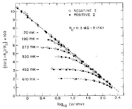
Figure 9. Resistivity as a function of voltage for a thin AuPd film, taken from [58]. The resistance $R_{0}=11.3$ M$\Omega$ corresponds to $R_{\Box}\approx 4500$ $\Omega$.

In order to explain the experiment Anderson et al. [59] argued that the logarithm as a function of voltage is directly related to the logarithm as a function of temperature (from weak localization in two dimensions) since the dissipated power heats the electron gas. In the case of a strong electric field, the electron temperature is of the order of the voltage drop on the relevant inelastic scattering length, the electron-phonon length, i.e. $T\sim eEL_{\rm e-ph}$, with $L_{\rm e-ph}=\sqrt{D\tau_{\rm e-ph}}$. Assuming $L_{\rm e-ph}$ to be proportional to a power of the temperature, $L_{\rm e-ph}\sim T^{-p}$, electric field and temperature are related as $T^{1+p}\sim E$ so that a logarithmic temperature dependence of the linear resistivity causes a logarithmic voltage dependence.

Shortly after the first experiments, it was discussed whether heating is the only origin of the non-linear conductivity, or if an electric field – in analogy to a magnetic field – can directly destroy weak localization via dephasing [60, 61]. The correct answer to the second question is “no” [62, 63], as one can easily verify by calculating the phase shifts of a pair of time reversed paths. In the presence of a vector potential an electron which propagates along a path ${\bf x}_{1}(t)$ or ${\bf x}_{2}(t)$ accumulates an additional phase

$$\varphi_{1,2}={e\over\hbar}\int_{0}^{\eta}{\rm d}t^{\prime}\dot{\bf x}_{1,2}\cdot{\bf A}.$$ (130)

For a pair of closed time-reversed paths, ${\bf x}_{2}(t)={\bf x}_{1}(\eta-t)$, and a static electric field, ${\bf A}(t)=-{\bf E}t$, the difference of the two phases vanishes, i.e. there is no “dephasing” from a static electric field.

However, in a successive study of the current-voltage characteristic of gold films, Bergmann et al. [64] noted that the experimental data are not completely compatible with a pure heating model. As a possible explanation of the experimental findings they suggested that the Coulomb interaction correction to the resistivity leads to a non-ohmic contribution, namely

$$\delta R_{\rm EEI}/R^{2}=-{e^{2}\over 4\pi^{2}\hbar}\ln\left[(k_{B}T)^{2}+\alpha\hbar D(eE)^{2}\right/k_{B}T],$$ (131)

where $\alpha$ is a factor of the order one.

Indeed in formulating the phase shift argument for the interaction contribution, a sensitivity to a static electric field cannot be excluded: The interaction correction to the conductivity is related to the propagation of a particle and a hole along closed paths. In the absence of a vector potential the phases of particle and hole cancel, whereas in the presence of a vector potential the accumulated phase difference is

$$\delta\varphi={e\over\hbar}\int_{t_{1}-\eta}^{t_{1}}{\rm d}t^{\prime}\dot{\bf x}_{1}\cdot{\bf A}-{e\over\hbar}\int_{0}^{\eta}{\rm d}t^{\prime}\dot{\bf x}_{2}\cdot{\bf A}.$$ (132)

As is shown in Fig. 8 the relevant paths obey the relations ${\bf x}_{1}(t)={\bf x}_{2}(t)$ for $0<t<t_{1}$ and ${\bf x}_{1}(t-\eta)={\bf x}_{2}(t)$ for $t_{1}<t<\eta$, which allows the phase difference to be written as

$$\delta\varphi={e\over\hbar}\int_{t_{1}-\eta}^{0}dt^{\prime}\dot{\bf x}_{1}\cdot[{\bf A}(t^{\prime})-{\bf A}(t^{\prime}+\eta)].$$ (133)

For the particular case of a static electric field described by ${\bf A}=-{\bf E}t$, this phase shift becomes $\delta\varphi={e\over\hbar}\eta({\bf x}_{2}-{\bf x}_{1})\cdot{\bf E}$. This suggests that the interaction correction should be sensitive to a static electric field, leading to a non-linear conductivity. The quantitative calculation in fact results in [27]

$$\delta R_{\rm EEI}/R^{2}\approx-{e^{2}\over 2\pi^{2}\hbar}\left(\ln k_{B}T+1.62{\hbar D(eE)^{2}\over(\pi k_{B}T)^{3}}\right),$$ (134)

verifying the non-ohmic behavior of the resistivity with the characteristic electric field scale as suggested in [64]. In order to derive Eq. (134), a thermal distribution function with electron temperature $T$ has been assumed. Following the steps in our calculation of the linear conductivity in section 4.1, Eq. (134) is obtained from (119) in two dimensions under the condition $\hbar D(eE)^{2}\ll(\pi k_{B}T)^{3}$. Note that the functional form (131) of the non-ohmic resistivity for strong electric fields cannot be confirmed theoretically. We remark, finally, that further theoretical results have been given in [27, 55], related to strong electric fields, time dependent fields, one to three dimensions, and magnetic field effects.

4.4. Gauge invariance

In the previous section we demonstrated that the non-linear electric field effect in the resistivity can be understood in terms of dephasing by calculating the phase shifts of the relevant classical paths in the presence of a time dependent vector potential. One may argue against this interpretation by noting that a vector potential can be gauged away in such a way that the static electric field is described by a static scalar potential, ${\bf E}({\bf x})=-\partial_{\bf x}\phi({\bf x})$. A static scalar potential does no longer affect the diffuson, so that the argument of the phase difference along two classical paths can no longer be used. In order to clarify the situation, we now verify explicitly the gauge invariance of the expression for the current density. First one notices that $\delta{\bf j}_{\rm Born}=-D\partial_{\bf x}\delta\rho$ is obviously gauge invariant. For $\delta{\bf j}_{V}$, on the other hand, an explicit check is necessary. Given the gauge transformation

$${\bf A} \to {\bf A}+\partial_{\bf x}\chi$$ (135)

$$\phi \to \phi-\partial_{t}\chi$$ (136)

the distribution function and the diffuson transform according to

$$F(\eta;{\bf x},t) \to F(\eta;{\bf x},t)\exp\{-{\rm i}e[\chi({\bf x},t+{\eta\over 2})-\chi({\bf x},t-{\eta\over 2})]\}$$ (137)

$$D^{\eta}({\bf x},t;{\bf x}^{\prime},t^{\prime}) \to D^{\eta}({\bf x},t;{\bf x}^{\prime},t^{\prime})$$ (138)

$$\times\exp\{-{\rm i}e[\chi({\bf x},t+{\eta\over 2})-\chi({\bf x},t-{\eta\over 2})]\}$$

$$\times\exp\{{\rm i}e[\chi({\bf x}^{\prime},t^{\prime}+{\eta\over 2})-\chi({\bf x}^{\prime},t^{\prime}-{\eta\over 2})]\}.$$

By applying the above transformation to $\delta{\bf j}_{V}$ as given in Eq. (115), one can easily verify that the function $\chi({\bf x},t)$ drops out, so that the expression is manifestly gauge invariant.

For the specific example of a static electric field with ${\bf A}=-{\bf E}t$ we choose $\chi({\bf x},t)=t{\bf E}\cdot{\bf x}$. After the gauge transformation the electric field appears in the distribution function, $\tanh(\epsilon/2T)\to\tanh[(\epsilon-\mu_{\bf x})/2T]$, $\mu_{\bf x}=e{\bf E}\cdot{\bf x}$, but not in the diffuson. We conclude that although the contribution of the Coulomb interaction to the current density is gauge invariant, the interpretation of the non-linear electric field effects depends on the actual choice of the potentials ${\bf A}$ and ${\bf\phi}$. With ${\bf E}=-\partial_{t}{\bf A}$, $\phi=0$ we would interpret the non-linear conductivity as due to a phase effect. With ${\bf E}=-\partial_{\bf x}\phi$, ${\bf A}=0$ the origin of the non-linear conductivity can be attributed to the varying local chemical potential which is felt by the traveling particle, and the virtual hole created and absorbed in the intermediate states.

4.5. Electron dephasing

The dephasing time sets the scale over which an electron propagates without loosing phase coherence, and determines the amplitude of the quantum interference corrections to the conductivity. Since elastic scattering does not destroy the electronic phase coherence, inelastic scattering must be hold responsible. Dephasing has been studied in much detail for weak localization [65, 66, 67, 68] (for a recent experimental review see [69]), and also in the context of universal conductance fluctuations [70, 71]. The amplitude of the interaction correction to the conductivity, on the other hand, is set by the thermal time $\tau_{T}=\hbar/k_{B}T$. In most cases the dephasing time is much longer than the thermal time. In some experiments, however, an extraordinarily strong phase breaking has been reported: Recently a low temperature saturation of $\tau_{\varphi}$ in gold wires [72, 73] has attracted much attention [23, 24, 25, 28, 74, 75, 76, 29]. Furthermore, in a number of cuprates, the dephasing rate decreases only slowly with decreasing temperature [77, 78, 79]. For example in $\rm Bi_{2}Sr_{2}CuO_{6}$, [77], the dephasing rate varies as $1/\tau_{\varphi}\sim T^{1/3}$, with $\tau_{\varphi}$ much shorter than $\tau_{T}$. In such a case phase breaking may become relevant also in the interaction contribution to the conductivity.

Unfortunately, in the experiments cited above, it is not clear which microscopic mechanism is responsible for the strong phase breaking. Nevertheless we believe it is important to answer the following questions: (i) Is phase breaking relevant in the interaction contribution to the conductivity? (ii) If yes, is the phase breaking rate which is relevant in the interaction contribution to the conductivity the same as for weak localization? While Castellani et al. [80] came to the conclusion that the answer is “yes” to both questions, Raimondi et al. [27] who reexamined the problem, confirmed the suggestion that dephasing is relevant also in the interaction contribution to the conductivity, but found a different dephasing time for the latter compared to weak localization. After some historical remarks we will give a semi-quantitative summary of the analysis carried out in [27].

While it is clear that inelastic scattering contributes to dephasing, the precise way this happens is less obvious. It was first noted by Schmid [81] that the inelastic quasi-particle scattering time is enhanced in the presence of disorder. The dephasing time was initially assumed to be identical to the inelastic quasi-particle scattering time [82], thus the inverse dephasing time was assumed to be $\propto T\ln T$ in two dimensions. Some time later, Fukuyama and Abrahams [66] reexamined the problem in terms of standard diagrams and calculated the “mass” that develops in the particle-particle propagator (the cooperon) in the presence of Coulomb interaction. They also found an inverse time proportional to $T\ln T$. Furthermore a mass term also appears in the particle-hole propagator (the diffuson) [80]. The mass in the particle-hole propagator turned out to coincide with that in the particle-particle propagator. However, calculating a mass is not sufficient in order to draw final conclusions; Altshuler, Aronov, and Khmelnitskii [65], for example, calculated the dephasing time via a path-integral approach and predicted an inverse dephasing time proportional to $T$, in contrast to [82]. This result – see also [67] – has been confirmed in many experiments. The approach of Altshuler, Aronov, and Khmelnitskii has been extended later in order to determine the relevant dephasings times for the universal conductance fluctuations [71], and in the particle-hole channel [27].

The general idea is that the phase of an electron which is propagating along a path ${\bf x}_{1,2}(t)$ is shifted by $\varphi_{1,2}={e}\int{\rm d}t\,\dot{\bf x}_{1,2}(t^{\prime})\cdot{\bf A}(t^{\prime})$. In the presence of fluctuating internal fields this results in phase fluctuations which finally destroys phase coherence. In thermal equilibrium the internal electric field fluctuations are given by

$$e^{2}\langle E^{i}E^{j}\rangle_{\bf q,\omega} = q^{i}q^{j}{{\rm i}\over 2}V^{K}({\bf q},\omega)$$ (139)

$$\approx -q^{i}q^{j}{2T\over\omega}{\rm Im}V^{R}({\bf q},\omega),$$ (140)

where $V^{K}({\bf q},\omega)$, $V^{R}({\bf q},\omega)$ are the Keldysh and the retarded Coulomb interaction, and low frequencies ($\omega\ll T$) have been assumed. The assumption of low frequencies is essential here since only in this frequency regime the classical field fluctuations, i.e. the Keldysh component of the interaction, dominates whereas at higher frequencies the nontrivial structure of the interaction in Keldysh space has to be taken into account. It has been shown by Fukuyama and Abrahams [66] and Castellani et al. [47] that the high frequency contributions of the Coulomb interaction renormalize parameters like the diffusion constant but do not contribute to dephasing. It is therefore reasonable to neglect these high frequency contributions in the following. The particle-particle propagator (cooperon) and the particle-hole propagator (diffuson) in the presence of the fluctuating field can then be written as a path-integral:

$$C^{t}_{\eta,\eta^{\prime}}({\bf x},{\bf x}^{\prime}) = {1\over 2}\int_{{\bf x}^{\prime}_{\eta^{\prime}}={\bf x}^{\prime}}^{{\bf x}_{\eta}={\bf x}}{\cal D}{\bf x}_{t_{1}}\exp-(S_{0}^{\rm p.p.}+S_{1}^{\rm p.p.})$$ (141)

$$D^{\eta}_{t,t^{\prime}}({\bf x},{\bf x}^{\prime}) = \int_{{\bf x}^{\prime}_{t^{\prime}}={\bf x}^{\prime}}^{{\bf x}_{t}={\bf x}}{\cal D}{\bf x}_{t_{1}}\exp-(S_{0}^{\rm p.h.}+S_{1}^{\rm p.h.})$$ (142)

with

$$S_{0}^{\rm p.p.}=\int_{\eta^{\prime}}^{\eta}{\rm d}t_{1}{\dot{\bf x}_{t_{1}}^{2}\over 2D},\quad S_{1}^{\rm p.p.}=-{\rm i}e\int_{\eta^{\prime}}^{\eta}{\rm d}t_{1}\dot{\bf x}_{t_{1}}\cdot[{\bf A}(t+t_{1}/2)+{\bf A}(t-t_{1}/2)]$$ (143)

$$S_{0}^{\rm p.h.}=\int_{\eta^{\prime}}^{\eta}{\rm d}t_{1}{\dot{\bf x}_{t_{1}}^{2}\over 4D},\quad S_{1}^{\rm p.h.}=-{\rm i}e\int_{\eta^{\prime}}^{\eta}{\rm d}t_{1}\dot{\bf x}_{t_{1}}\cdot[{\bf A}(t_{1}+\eta/2)-{\bf A}(t_{1}-\eta/2)].$$ (144)

In both cases the $S_{1}$ term describes the additional phase due to the vector potential ${\bf A}$. Since we have to consider the phase difference of pairs of classical paths, the vector potential appears twice in $S_{1}$. In the case of the cooperon the two paths are the time reversed of the other, i.e., to a velocity $\dot{\bf x}$ on path “$1$” corresponds a velocity $-\dot{\bf x}$ on path “$2$” and in the expression for the phase difference the sum of two vector potentials appears. In the case of the diffuson the two paths are traversed in the same direction, but at different times. Therefore the minus sign between the two vector potentials remains, and in particular when the two paths are traversed at the same time ($\eta=0$) the phase difference vanishes. By averaging the phase factor $\exp(-S_{1})$ over the electric field fluctuations, using the relation

$$\langle\exp({\rm i}\delta\varphi)\rangle=\exp\left(-{1\over 2}\langle(\delta\varphi)^{2}\rangle\right)\equiv\exp(-S),$$ (145)

one finds

$$S^{\rm p.p.} = {1\over 2}\int_{-\eta}^{\eta}\!{\rm d}t_{1}\int_{-\eta}^{\eta}\!{\rm d}t_{2}\int_{-T}^{T}{{\rm d}\omega\over 2\pi}\sum_{\bf q}{2T\over\omega}\left[-{\rm Im}V^{R}({\bf q},\omega)\right]$$ (146)

$$\times \exp\left\{{\rm i}{\bf q}\cdot[{\bf x}_{1}(t_{1})-{\bf x}_{1}(t_{2})]\right\}\left[\cos\left(\omega{t_{1}-t_{2}\over 2}\right)-\cos\left(\omega{t_{1}+t_{2}\over 2}\right)\right]$$ (147)

in the case of the cooperon, and

$$S^{\rm p.h.} = \int_{0}^{\eta}\!{\rm d}t_{1}\int_{0}^{\eta}\!{\rm d}t_{2}\int_{-T}^{T}{{\rm d}\omega\over 2\pi}\sum_{\bf q}{2T\over\omega}\left[-{\rm Im}V^{R}({\bf q},\omega)\right]$$ (148)

$$\times \exp\left\{{\rm i}{\bf q}\cdot[{\bf x}_{1}(t_{1})-{\bf x}_{1}(t_{2})]\right\}{\rm e}^{-{\rm i}\omega(t_{1}-t_{2})}\left[1-\cos(\omega\eta)\right]$$ (149)

in the case of the diffuson; in both $S^{\rm p.p.}$ and $S^{\rm p.h.}$ the velocities $\dot{\bf x}(t_{1,2})$ were removed by a partial integration, and the relation between the two relevant paths ${\bf x}_{1}(t)$ and ${\bf x}_{2}(t)$ was exploited. The expressions for $S^{\rm p.p.}$ and $S^{\rm p.h.}$ appear to be similar, except for the time dependent factors in the second line; this leads to different dephasing times in the particle-particle and particle-hole channels. In two dimensions, for example, the final results are

$$S^{\rm p.p.}\approx(T\eta){R_{\Box}\over h/e^{2}}\ln(T\eta);\,\,\,\,{1\over\tau_{\varphi}}\approx T{R_{\Box}\over h/e^{2}}\ln\left({h/e^{2}\over R_{\Box}}\right)$$ (150)

and

$$S^{\rm p.h.}\approx(T\eta){R_{\Box}\over h/e^{2}}\ln(D\kappa^{2}T\eta^{2});\,\,\,\,{1\over\tau_{\varphi}}\approx T{R_{\Box}\over h/e^{2}}\ln\left[{D\kappa^{2}\over T}\left({h/e^{2}\over R_{\Box}}\right)^{2}\right],$$ (151)

where $\kappa$ is the inverse screening length, and $R_{\Box}$ is the sheet resistance. The dephasing time is here determined from the condition $S(\eta\!=\!\tau_{\varphi})=1$. In the particle-particle channel the standard result of Altshuler, Aronov and Khmelnitskii [65, 67, 68] is confirmed. The dephasing time in the particle-hole channel is finite, different from the one in the particle-particle channel, and is identical to the inelastic scattering rate in the two-particle propagators (diffuson or cooperon), as first calculated by Fukuyama and Abrahams [66, 84].

The low frequency electric field fluctuations considered here, cannot explain the strong phase breaking observed in [72, 77]. However we expect similar results for other phase breaking mechanisms: We suggest that a mechanism leading to strong dephasing in the particle-particle channel will also cause strong dephasing in the particle-hole channel. In particular when $\tau_{\varphi}$ becomes comparable to or shorter than the thermal time $\tau_{T}$, the relevant time scale which sets the amplitude of the Coulomb interaction contribution to the conductivity will be $\tau_{\varphi}$ instead of $\tau_{T}$. This is consistent with the experiments: In the gold wires of [72] the dephasing rate saturated below $T\sim 1$ K to values of the order of $\hbar/\tau_{\varphi}\sim 1$-$10$ mK. In the samples with the strongest phase breaking a saturation of the interaction correction to the conductivity has been observed below $T\sim 100$ mK [73]. In $\rm Bi_{2}Sr_{2}CuO_{6}$, a compound with a single $\rm CuO_{2}$ plane per unit cell, the in-plane zero field resistivity increases as $\ln T$ below $\sim$18 K, consistent with quantum interference effects in two dimensions. The shape of the orbital magneto-resistance is well fitted by the weak localization expression [77], but with an unexpected large dephasing rate which varies as $T^{1/3}$. The spin component of the magneto-resistance varies at low fields as $[R(B)-R(0)]/R(0)\sim(B/B_{s})^{2}$. From the standard theory for the Coulomb interaction in the spin triplet channel [83, 15] one would expect such a quadratic magnetic field dependence with a magnetic field scale which is linear in the temperature, $B_{s}\sim 1/\tau_{T}$. Experimentally the magnetic field scale varies as $T^{0.4}$, which is close to the temperature variation of the dephasing rate. This suggests that the origin of the spin component of the magneto-resistance might indeed be the Coulomb interaction contribution to the conductance, but in the presence of an up to now unidentified phase breaking mechanism.

5. The Coulomb interaction in nanostructures

Quasiclassical methods – as pioneered by Nazarov – allow description of interaction effects in a unified way. For instance, in the following subsection we will show that Coulomb blockade physics in small tunnel junctions and disorder-induced zero-bias anomalies in diffusive conductors are closely related. More generally the question arises how the Coulomb interaction affects the transport in small systems with diffusive electron motion, where interfaces provide an additional source of scattering. Typical situations will be examined in detail in the subsequent subsections.

5.1. Coulomb interaction and interface conductance

The Coulomb interaction plays an important role not only in diffusive transport, but also for transport across interfaces. For example, the Coulomb interaction reduces the density of states near the Fermi energy, [20, 21, 103, 46, 47, 85, 86, 51] which leads to a suppression of the transmission of tunnel junctions, and to a non-linear current-voltage characteristic at low bias. On the other hand Coulomb blocking of tunneling may also be due to interface charging effects [87, 88, 89, 90, 91]. These two classes of phenomena were described in a unified way for the first time by Nazarov [92, 93], and later by various authors [85, 95, 96, 97, 98, 99, 100].

In this subsection we will show how to construct the theory within the quasiclassical scheme. Whereas in the above cited references it is assumed that the electronic system on both sides of the interface is in thermal equilibrium, there is no such assumption in the approach we present here. The idea is to start with the boundary conditions for the quasiclassical Green’s function, derive an expression for the current through the interface, and at the end average over the fluctuations of the internal electric field.

Zaitsev’s boundary condition [101, 102], which generalizes the matching condition (57) to situations where $g^{R,A}\neq\pm 1$, reads

$$\check{a}\left[R-R\check{a}\check{a}+{T\over 4}(\check{s}({\bf x}_{-})-\check{s}({\bf x}_{+}))^{2}\right]={T\over 4}[\check{s}({\bf x}_{+}),\check{s}({\bf x}_{-})]$$ (152)

with

$$\check{s} = {1\over 2}\left[\check{g}(\hat{\bf p})+\check{g}(\tilde{\hat{\bf p}})\right]$$ (153)

$$\check{a} = {1\over 2}\left[\check{g}(\hat{\bf p})-\check{g}(\tilde{\hat{\bf p}})\right].$$ (154)

The antisymmetric combination of Green’s functions $\check{a}$ is continuous across the interface. In the absence of electronic interactions ($g^{R,A}=\pm 1$), we recover Eq. (57). In the interacting case, where $g^{R,A}\neq\pm 1$, we restrict our considerations to the limit of low interface transparency, $T/R\ll 1$ . Then the structure of the boundary conditions becomes simple,

$$a^{K}={T\over 4}[\check{s}({\bf x}_{+}),\check{s}({\bf x}_{-})]^{K},$$ (155)

and the current density across an interface which connects two dirty pieces of metal is given by

$$\hat{\bf n}\cdot{\bf j} = e\pi N_{0}\Gamma{1\over 2}\int{{\rm d}\epsilon\over 2\pi}\langle\left[\check{g}_{s}({\bf x}_{+}),\check{g}_{s}({\bf x}_{-})\right]^{K}\rangle_{\phi^{\rm int}}$$ (156)

$$\Gamma = v_{F}{1\over 2}\int_{0}^{1}{\rm d}(\cos\theta)\cos\theta\,T(\cos\theta).$$ (157)

In the absence of interactions the tunneling conductivity of the interface is given by $\sigma_{T}=2e^{2}N_{0}\Gamma$. The remaining technical difficulty in order to evaluate the current through an interface in the presence of interactions is the average over the internal field fluctuations. Solutions are known only in some special situations; one of these is when the two sides of the interface are uncorrelated such that the average over the internal field fluctuations factorizes. The current can then be written in a familiar form in terms of the local density of states $N(\epsilon,{\bf x})$ as

$$\hat{\bf n}\cdot{\bf j} = e{\Gamma\over N_{0}}\int{{\rm d}\epsilon}\left[F(\epsilon,{\bf x}_{-})-F(\epsilon,{\bf x}_{+})\right]N(\epsilon,{\bf x}_{+})N(\epsilon,{\bf x}_{-})$$ (158)

$$N(\epsilon,{\bf x}) = \pm N_{0}{\rm Re}\langle g^{R,A}(\epsilon,{\bf x})\rangle_{\phi^{\rm int}}.$$ (159)

In general, however, such correlations do exist due to the interaction between the electrons on opposite sides of the interface.

Another situation where Eq. (156) can be evaluated explicitly is when the gradients in the kinetic equation on both sides of the interface are negligible, i.e. when the diffusive motion of the charge carriers is negligible. In this limit standard Coulomb blockade theory ($P(E)$ theory, [57]) is recovered as we demonstrate here. The question under which circumstances the gradient terms in the kinetic equation can be neglected will not be addressed here: For a discussion of this issue see the appendix of [57], and also subsection 5.4. Neglecting the gradient term, the kinetic equation in the presence of the Coulomb interaction can be solved explicitly, and the Green’s function reads

$$\check{g}_{t_{1}t_{2}}({\bf x})={\rm e}^{{\rm i}\check{\varphi}(t_{1},{\bf x})}\check{g}_{0,t_{1}t_{2}}({\bf x}){\rm e}^{-{\rm i}\check{\varphi}(t_{2},{\bf x})},$$ (160)

with $\partial_{t}\check{\varphi}=e\check{\phi}_{\rm int}$, and $\check{g}_{0}$ is the Green’s function in the absence of the interaction. Since we assume Gaussian fluctuations for the internal field $\phi_{\rm int}$, it is clear that the average over $\phi_{\rm int}$ can be carried out for both the Green’s functions and the current density, Eq. (156). The final result for the current density can be written in the form

$$\hat{\bf n}\cdot{\bf j} = e2\Gamma N_{0}\int{{\rm d}\epsilon}\int{\rm d}\omega P(\omega)$$ (162)

$$\times\left\{f(\epsilon,{\bf x}_{+})[1-f(\epsilon-\omega,{\bf x}_{-})]-f(\epsilon,{\bf x}_{-})[1-f(\epsilon-\omega,{\bf x}_{+})]\right\}$$

with $F(\epsilon,{\bf x})=1-2f(\epsilon,{\bf x})$. The factors $f(\epsilon,{\bf x}_{+})[1-f(\epsilon-\omega,{\bf x}_{-})]$ describe the tunneling of a charge from an occupied state on the “$+$”-side of the junction to an unoccupied state on the “$-$”-side. In the absence of interactions the function $P(\omega)$ is a delta function centered at zero, and the usual expression for the tunnel current is obtained. In the presence of interactions a tunneling electron may exchange energy with the environment, and $P(\omega)$ may be interpreted as the probability to transfer the energy $\omega$ to the environment [57]. The function $P(\omega)$ is given by

$$P(\omega) = {1\over 2\pi}\int{\rm d}t{\rm e}^{{\rm i}\omega t}{\rm e}^{J(t)}$$ (163)

$${J(t)} = \langle(\varphi_{1}(t)-\varphi_{1}(0))\varphi_{1}(0)\rangle_{\phi_{\rm int}}+\langle\varphi_{1}(t)\varphi_{2}(0)\rangle_{\phi_{\rm int}}-\langle\varphi_{2}(t)\varphi_{1}(0)\rangle_{\phi_{\rm int}},$$ (164)

where $\varphi_{1,2}$ is the phase difference between the left and right leads, $\varphi_{1,2}=\varphi_{1,2}({\bf x}_{-})-\varphi_{1,2}({\bf x}_{+})$; the index $1,2$ refers to the Keldysh space. In thermal equilibrium and expressing the phase/voltage fluctuations over the junction in terms of an impedance $Z$ one has

$$\int{\rm d}t{\rm e}^{{\rm i}\omega t}\langle\varphi_{1}(t)\varphi_{2}(0)\rangle_{\phi_{\rm int}}={1\over 2}{e^{2}Z\over\omega};$$ (165)

the function $J(t)$ is determined as

$$J(t)=\int{{\rm d}\omega\over\omega}{{\rm Re}Z\over 2\pi/e^{2}}\left\{\left[\cos(\omega t)-1\right]\coth\left(\omega\over 2T\right)-{\rm i}\sin(\omega t)\right\}.$$ (166)

As an example, to mimic the electrodynamic environment of a tunnel junction, assume the impedance $Z$ to be $Z=1/(-{\rm i}\omega C+R^{-1})$, i.e. a capacitance in parallel with a resistor. For a high impedance, $R\gg h/e^{2}$, when the charge relaxation process becomes slow, one obtains

$$J(t)=-{\rm i}E_{c}t-E_{c}Tt^{2},$$ (167)

where $E_{c}=e^{2}/2C$ is the charging energy. In the zero temperature limit $P(\omega)$ reduces to a delta function,

$$P(\omega)=\delta(\omega-E_{c}),$$ (168)

such that a minimum voltage difference $E_{c}/e$ is needed for an electron to tunnel through the junction. The current-voltage characteristic is given by

$$I(V)=G_{T}(V-E_{c}/e)\Theta(eV-E_{c}),\quad G_{T}=2e^{2}N_{0}\Gamma{\cal A}.$$ (169)

For more applications of the standard Coulomb blockade theory we refer to the literature, e.g. [91].

We close this subsection by highlighting how the zero-bias Altshuler-Aronov anomalies arise. These are present in situations where the gradient in the kinetic equation cannot be neglected. Since under this condition an exact expression for the Green’s function near the junction is not known, we restrict ourselves to a pertubative expansion in the internal field $\check{\phi}_{\rm int}$, with the result

$$\hat{\bf n}\cdot\delta{\bf j} = -e\pi N_{0}\Gamma{1\over 2}\int{{\rm d}\epsilon\over 2\pi}\left[F(\epsilon,{\bf x}_{-})-F(\epsilon,{\bf x}_{+})\right]$$ (170)

$$\times\Big{[}{\rm Re}\langle\delta g^{K}({\bf x}_{+})[\delta g^{Z}({\bf x}_{+})-\delta g^{Z}({\bf x}_{-})]\rangle_{\phi^{\rm int}}$$

$$+{\rm Re}\langle\delta g^{K}({\bf x}_{-})[\delta g^{Z}({\bf x}_{-})-\delta g^{Z}({\bf x}_{+})]\rangle_{\phi^{\rm int}}\Big{]},$$

where $\delta g^{K}$ and $\delta g^{Z}$ are the correction to the Green’s functions due to the fluctuating field. The relevant correlation function has been given in Eq. (112), and we find

$$\hat{\bf n}\cdot\delta{\bf j} = {1\over 2e}\sigma_{T}\int{\rm d}\epsilon\left[F(\epsilon,{\bf x}_{-})-F(\epsilon,{\bf x}_{+})\right]{\rm Im}\int{{\rm d}\omega\over 2\pi}\int{\rm d}{\bf x}_{1}F(\epsilon-\omega,{\bf x}_{1})$$ (171)

$$\times\left\{\rho_{0}({\bf x}_{+},\omega;{\bf x}_{1})\left[\phi_{\rm ind}({\bf x}_{1},\omega;{\bf x}_{+})-\phi_{\rm ind}({\bf x}_{1},\omega;{\bf x}_{-})\right]\right.$$

$$\left.+\rho_{0}({\bf x}_{-},\omega;{\bf x}_{1})\left[\phi_{\rm ind}({\bf x}_{1},\omega;{\bf x}_{-})-\phi_{\rm ind}({\bf x}_{1},\omega;{\bf x}_{+})\right]\right\},$$

where $\sigma_{T}$ is the tunneling conductivity in the absence of interactions, $\rho_{0}({\bf x},{\bf x}^{\prime})$ and $\phi_{\rm ind}({\bf x},{\bf x}^{\prime})$ are the charge density and the induced electrical potential at ${\bf x}$ due to a charge which is generated at ${\bf x}^{\prime}$, compare subsection 4.2. When interactions are taken into account only on one side of the interface, the correction to the current is controlled by the density of states. For example in three dimensions the correction to the density of states is proportional to $\sqrt{\epsilon}$, giving rise to a $\sqrt{V}$ of the tunneling conductivity as a function of voltage [13]. However, in the more general situation, as pointed out by Nazarov [92, 93], correlations in both leads and between the leads have to be taken into account.

For further experiments where the perturbative zero bias anomalies in the tunnel conductivity have been observed, see for example [96, 97, 98]. We will work out the Coulomb correction (171) to the interface current for a specific geometry in section 5.3.

5.2. Non-linear conductivity in wires

In this and the following two subsections we will discuss the contribution of the Coulomb interaction to the conductivity in small systems. We would like to mention that size effects in the quantum corrections to the linear conductivity were studied in detail in the mid-eighties [103, 104, 105]. In contrast, we will focus here on the case of a large applied voltage. We will successively decrease the size of the systems under consideration. This subsection is devoted to wires which may be shorter than the inelastic scattering length, but which are still longer than the thermal diffusion length $L_{T}=\sqrt{\hbar D/k_{B}T}$. This is then followed by subsection 5.3 where we consider system sizes of the order of $L_{T}$. There it will be essential to consider the discreteness of the diffusive modes, and we will also allow for resistive interfaces between the wire and the leads. Finally, in subsection 5.4 we will consider the situation of a small, fully coherent piece of metal beeing connected to two large reservoirs.

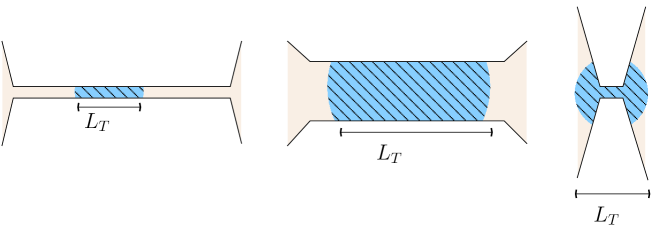
Figure 10. The geometries considered in subsections 5.2 – 5.4. Section 5.2 is devoted to wires which are much longer than the thermal diffusion length $L_{T}$. In Sec. 5.3 $L_{T}$ is of the order of the system size; both in Sec. 5.2 and Sec. 5.3 we assume ideal leads. In section 5.4 a diffusive point contact is considered, where the system size is much smaller than $L_{T}$ such that the phase coherent volume extends into the leads, which then have to be taken into account explicitly.

We start with a long, thin wire, for which the Coulomb correction to the resistivity, including the leading non-linear voltage dependence, in analogy to Eq. (134) for a thin film, is given by [55]

$$\delta R_{\rm EEI}/R^{2}\approx{e^{2}\over\pi^{2}\hbar}{L_{T}\over L}\left(4.91-0.21{\hbar D(eV/L)^{2}\over(k_{B}T)^{3}}\right),$$ (172)

where $V=EL$ is the applied voltage. Again, this result has been obtained under the assumption of a thermal distribution function with a constant temperature $T$. Whereas this is reasonable for macroscopic samples, it fails, however, in samples which are shorter than the electron-phonon scattering length, in which case the Coulomb interaction correction to the conductivity far from equilibrium [56, 106, 54] has to be considered.

For an evaluation of the current-voltage characteristic, the diffuson and the distribution function in the wire are required. The diffuson is found by solving the differential equation (110) with the condition that the derivative normal to an insulating boundary (i.b.) vanishes, i.e.

$$(\hat{\bf n}\cdot\nabla_{\bf x})D({\bf x},{\bf x}^{\prime}){\big{|}}_{{\bf x}\,\in{\rm\,i.b.}}=0,$$ (173)

while the diffuson itself vanishes at a metallic boundary (m.b.),

$$D({\bf x},{\bf x}^{\prime}){\big{|}}_{{\bf x}\,\in{\rm\,m.b.}}=0.$$ (174)

The first condition means that no current flows through the interface, the second condition corresponds to the assumption that an electron arriving at the metallic boundary escapes into the leads with zero probability to come back into the wire. Furthermore it is assumed that the left and right leads of the wire are in thermal equilibrium,

$$F(\epsilon,{\bf x}){\big{|}}_{{\bf x}\,\in\,l.l.,r.l.}=\tanh\left({\epsilon\pm|e|V/2\over 2T}\right).$$ (175)

By solving the kinetic equation it is found that the distribution function depends on the various relaxation mechanisms governing the collision integral [107, 108, 109, 110, 24], and we distinguish three regimes:

• When the system is much longer than the electron-phonon scattering length, $L\gg L_{\rm e-ph}$, the distribution function acquires the equilibrium form with a local chemical potential and temperature,

  $$F(\epsilon,x)=\tanh\left({\epsilon+|e|V(L-2x)/2L\over 2T_{e}(x,V)}\right),$$ (176)

  where $x=0\dots L$ is the distance from the left lead. The local electron temperature $T_{e}(x)$ may be determined from an energy balance argument, assuming that the dissipated power equals the gradient of the heat flow. In the limit considered here the heat flow is dominated by the phonons. For a stationary temperature $T_{e}(V)$ the Joule heating power $P_{\rm in}=\sigma{\bf E}^{2}$ equals the power which is transferred into the phonon system, $P_{\rm out}$. For weak heating one has $P_{\rm out}=c_{V}\Delta T/\tau_{\rm e-ph}$, where $c_{V}$ is the electron specific heat, $\Delta T$ is the difference between the electron and phonon temperatures, and $\tau_{\rm e-ph}$ is the relevant energy relaxation rate. For strong heating, on the other hand, the effective electron temperature is of the order of the voltage drop over a phonon length, $T_{e}\sim|e|VL_{\rm e-ph}/L$. If the “hot” phonons escape ballistically into the substrate, the temperature in the bulk of the wire does not depend on the position $x$ but is voltage dependent, $T_{e}=T_{e}(V)$. By neglecting the region near the leads, where the temperature rises from $T_{\rm lead}$ to $T_{e}(V)$, Eq. (172) is recovered for the voltage dependent resistivity.

• When $L_{\rm e-ph}\gg L\gg L_{\rm in}$ one still expects a distribution function near local equilibrium, due to electron-electron scattering. The local temperature is determined from the relation $\sigma E^{2}=$$-\nabla[\kappa\nabla T_{e}(x)]$, where $\kappa$ is the thermal conductivity. Using the Wiedemann-Franz law, $\kappa=({\pi^{2}/3})$ $T_{e}\sigma(k_{B}/e)^{2}$, the temperature profile in the wire is determined as

  $$T_{e}^{2}(x)=T_{\rm lead}^{2}+{3\over\pi^{2}}\left({eV\over L}\right)^{2}x(L-x).$$ (177)

• In the absence of inelastic scattering, realized when $L_{\rm in}\gg L$, the distribution function is a linear superposition of the distribution function of the leads,

  $$F(\epsilon,x)=\left[(L-x)F(\epsilon,0)+xF(\epsilon,L)\right]/L.$$ (178)

The resistance as a function of voltage in regime a) is given in Eq. (172). This equation applies when the voltage drop over a thermal diffusion length is smaller than the temperature, $eVL_{T}/L<T$. Since we assume that $L_{\rm e-ph}>L$ the electron temperature as a function of voltage rises so fast that this condition always holds. We compare now the relative importance of both heating and non-heating effects for the non-linear resistivity. From the linear conductivity and the increase of temperature due to the applied voltage as discussed above, we find at low voltage

$$\delta R_{\rm heating}/R^{2}\approx-4.91{e^{2}\over\pi^{2}}{L_{T}\over L}{D(eV/L)^{2}\over T^{2}(1/\tau_{\rm e-ph})},$$ (179)

which has to be compared with the corresponding change of the resistance due to non-heating effects:

$$\delta R_{\rm non-heating}/R^{2}\approx-0.21{e^{2}\over\pi^{2}}{L_{T}\over L}{D(eV/L)^{2}\over T^{3}}.$$ (180)

One observes that the heating contribution to the non-linear resistivity is larger by a factor $T\tau_{\rm e-ph}$. Thus the non-heating effects are difficult to observe experimentally, since usually $1/\tau_{\rm e-ph}\ll T$.

We now consider the other two limits, b) and c). We found that in both limits the current can be written as [54]

$$\delta I_{\rm EEI}(V,T)={e^{2}\over\hbar}{L_{T}\over L}f\left({eV/k_{B}T}\right)V,$$ (181)

where the function $f$ depends on the distribution function and on the length of the wire; $T$ is the temperature in the leads. Numerical results are shown in Fig. 11. Notice that $f(eV/k_{B}T)$ is proportional to $\delta I_{\rm EEI}/V$, so that $f(eV/k_{B}T)$ also represents the voltage dependent conductance in units of $(e^{2}/\hbar)(L_{T}/L)$.

Figure 11. Interaction correction to the conductance $\delta I_{\rm EEI}/V$ for a mesoscopic wire as a function of voltage, taken from [54]. $\delta I_{\rm EEI}/V$ is plotted in units of $(e^{2}/\hbar)L_{T}/L$. The full line corresponds to the non-equilibrium distribution function (178). The line with long dashes corresponds to the local equilibrium distribution function (176) with $x$-dependent temperature. The line with short dashes ($L/L_{T}=5$) is the non-linear conductivity due to the heating contribution only, Eq. (183).

For low voltage and large system size $L\gg L_{T}$, the result [103]

$$\delta I_{\rm EEI}/V\approx-{e^{2}\over\hbar}{L_{T}\over L}\left[{3\zeta(3/2)\over(2\pi)^{3/2}}-{5\over 6}{L_{T}\over L}+{5\sqrt{2}\zeta(5/2)\over\pi^{5/2}}{L_{T}^{2}\over L^{2}}+\dots\right];\quad{3\zeta(3/2)\over(2\pi)^{3/2}}\approx 0.498$$ (182)

is approached. With decreasing length the correction to the current decreases, since electrons escape more quickly from the wire into the leads. The full lines show the voltage dependent conductance for case c); the long-dashed line corresponds to case b). The short-dashed line ($L/L_{T}=5$) is obtained within a simple approximation: Instead of evaluating the full expression for $\delta{\bf j}_{\rm EEI}$ we take the linear conductivity as a function of temperature, and average over the temperature profile,

$$\delta\sigma_{\rm heating}={1\over L}\int_{0}^{L}\!{\rm d}x\,\delta\sigma(T(x)).$$ (183)

Important results are the following: in both cases b) and c) the conductance scales with voltage over temperature. In case b) (hot electrons) the main effect is simple heating, i.e. the non-ohmic effects are small. In case c) (far from equilibrium) the current-voltage characteristic is quantitatively different from the hot electron regime. The temperature dependence of the Coulomb interaction contribution to the conductance is shown in Fig. 12 in a double logarithmic plot. The curves shown are obtained from the same numerical data for $f(eV/k_{B}T)$ as shown in Fig. 11 ($L/L_{T}=200$).

Figure 12. Temperature dependence of the Coulomb interaction correction to the conductance of a mesoscopic wire in arbitrary units. The full line corresponds to the double-step distribution function, the dashed line corresponds to hot electrons with temperature profile, as explained in the text; $T$ is the electron temperature in the reservoirs.

At high temperature the Coulomb correction to the conductance follows $1/\sqrt{T}$, which is seen as a linear behavior in the double logarithmic plot. When the temperature in the leads becomes lower than the voltage, the conductance saturates. In the absence of inelastic scattering, c), this low temperature saturation appears at a higher temperature than in b).

Finite size effects in the linear conductivity of thin wires of length $L\sim L_{T}$ have been studied e.g. by Masden and Giordano [104] who found a qualitative (although not quantitative) agreement with the theoretical predictions. The distribution function in mesoscopic wires out of thermal equilibrium was measured by Pothier et al. [111]. For short wires and low temperature ($L\approx 1.5$ $\mu$m, $T\approx 25$ mK), the double step like distribution function was observed. Unfortunately, as far as we know, there is no detailed investigation of the temperature and voltage dependence of the conductivity in this experiment.

5.3. Short wire with interfaces

In subsection 2.4 we demonstrated how to obtain the classical resistance of a system which is composed of diffusive pieces and resistive interfaces in the framework of the quasiclassical description. In this subsection, following closely [112], we include the Coulomb interaction, and in particular we will concentrate on structures of a size comparable to the thermal diffusion length $L_{T}$. In subsection 5.1 we described a general formalism to obtain the quantum correction to the current through an interface; here we apply the formalism to a specific geometry where a diffusive piece of metal is connected via resistive interfaces to a left ($x=0$) and right ($x=L$) reservoir.

We divide the quantum correction to the current into two contributions: The first has the meaning of a correction to the conductance, $\delta I^{(1)}=V\delta G$. The second can be interpreted as the redistribution of the voltage across the interfaces and the wire, $\delta I^{(2)}=G\delta V$. More precisely we denote by $\delta I^{(2)}$ those terms which arise from the correction to the distribution function like, for example,

$$\delta I^{(2)}_{\rm wire}=-eDN_{0}{\cal A}\int{\rm d}\epsilon\,\partial_{\bf x}\delta F(\epsilon;{\bf x});$$ (184)

we will give the explicit expression for $\delta I^{(1)}_{\rm wire}$ below. Both terms are necessary in order to ensure current conservation. In principle the variation of the distribution function, $\delta F(\epsilon;{\bf x})$, can be determined by solving the kinetic equation in the presence of interactions. However by exploiting current conservation it appears that this is not necessary. For the time independent problem which we consider here, current conservation means that the current does not depend on the position, i.e. $I_{l}=I_{\rm wire}=I_{r}$, where the subscripts $l$ and $r$ indicate the left and right interface. By fixing the voltage drop over the whole system to $V$, such that the sum $\delta V_{l}+\delta V_{r}+\delta V_{\rm wire}$ is zero, it is possible to eliminate $\delta I^{(2)}$ from the equations to obtain the correction to the current as

$$\delta I_{\rm EEI}={R_{l}\delta I_{l}^{(1)}+R_{r}\delta I_{r}^{(1)}+R_{\rm wire}\delta I_{\rm wire}^{(1)}\over R_{l}+R_{r}+R_{\rm wire}}.$$ (185)

To proceed further we need the explicit form of $\delta I^{(1)}_{l,r,{\rm wire}}$. For an interface which is attached to an ideal lead on one side, the quantum correction to the current is controlled by the correction to the density of states on the other side,

$$\delta I_{l}^{(1)} = -e{\cal A}\Gamma_{l}\int{\rm d}\epsilon\delta N(\epsilon,0)[F(\epsilon;0)-F^{l}(\epsilon)]$$ (186)

$$\delta I_{r}^{(1)} = -e{\cal A}\Gamma_{r}\int{\rm d}\epsilon\delta N(\epsilon,L)[F^{r}(\epsilon)-F(\epsilon;L)].$$ (187)

Quite generally we obtain the density of states correction as

$$\delta N(\epsilon,{x}) = -N_{0}\int{{\rm d}\omega\over 2\pi}S({x},{x})$$ (188)

$$S({x},{x}) = -{\rm Im}\int{\rm d}{x}_{1}$$ (190)

$$\times F({\epsilon-\omega};{x}_{1})\rho_{0}({x},\omega;{x}_{1})\phi_{\rm ind}({x}_{1},\omega;{x}),$$

where $\rho_{0}({x},\omega;{x}_{1})$ describes the spreading of a charge injected into the system at ${x}_{1}$, and $\phi_{\rm ind}$ is the induced electrical potential as we discussed in subsection 4.2. By using the same notation for the correction to the current in a diffusive wire we find

$$\delta I_{\rm wire}^{(1)}(x) = eDN_{0}{\cal A}\int{\rm d}\epsilon\int{{\rm d}\omega\over 2\pi}\partial_{x}[F(\epsilon;x)S(x,x)]$$

$$-2eDN_{0}{\cal A}\int{\rm d}\epsilon\int{{\rm d}\omega\over 2\pi}F(\epsilon;x)\partial_{x_{1}}S(x,x_{1})|_{x_{1}=x}.$$

In general $\delta I_{\rm wire}^{(1)}(x)$ depends on the position $x$. Equation (185), however, is constructed in such a way that the spatial average $\delta I_{\rm wire}^{(1)}=L^{-1}\int{\rm d}x\delta I_{\rm wire}^{(1)}(x)$ has to be inserted.

We have already discussed the distribution function $F$ including the relevant boundary conditions in subsection 2.4. Inside a diffusive wire the charge density $\rho_{0}$ satisfies the diffusion equation, Eq. (125). At the boundaries to the left and right reservoir, one may derive the matching conditions

$$D\partial_{x}\rho_{0}(\omega,x;x^{\prime})|_{x=0} = \Gamma_{l}\rho_{0}(\omega,0;x^{\prime})$$ (192)

$$D\partial_{x}\rho_{0}(\omega,x;x^{\prime})|_{x=L} = -\Gamma_{r}\rho_{0}(\omega,L;x^{\prime}),$$ (193)

to be compared with the boundary conditions for the distribution function, Eqs. (62) and (63). A careful analysis is also required for the induced field $\phi_{\rm ind}(\omega,{x};{x}^{\prime})$. We assume good metallic screening (compare subsection 4.2) so that an injected charge is almost instantly screened, and therefore the wire will be electrically neutral with the possible exception of a thin surface layer. In this case inside the wire, one has

$$-\sigma\partial_{x}^{2}\phi_{\rm ind}(\omega,{x};{x}^{\prime})=e\delta({x}-{x}^{\prime}),$$ (194)

where $\sigma=2e^{2}DN_{0}{\cal A}$ is the conductivity.

From now on we concentrate on a short resistive wire with interfaces assuming temperatures of the order of and lower than the Thouless energy, $\hbar D/L^{2}$.

Figure 13. Contribution of the electron-electron interaction to the temperature dependence of the conductance of a wire with length $L\sim L_{T}$ for different values of the bias voltage, from [112]. The results are obtained under the assumption that the charge diffusion can be described with just a single diffusive mode. $\partial I/\partial V$ is in units of $e^{2}/h$ and must be multiplied with the non-universal number $A$ defined in the Eq. (197). $\gamma_{0}$ is the energy of the lowest diffusive mode; in the absence of interface barriers $\gamma_{0}=\pi^{2}\hbar D/L^{2}$, for strongly resistive interfaces $\gamma_{0}\to 0$.

We start by expanding the charge density $\rho_{0}$ in diffusive modes,

$$\rho_{0}(\omega,x;x^{\prime}) = e\sum_{n}{f_{n}(x)f_{n}(x^{\prime})\over-{\rm i}\omega+\gamma_{n}},$$ (195)

where the (normalized) functions $f_{n}(x)$ are obtained from the eigenvalue equation

$$-D\partial_{x}^{2}f_{n}(x)=\gamma_{n}f_{n}(x).$$ (196)

In the zero-dimensional limit we approximate the sum in Eq. (195) by retaining only the eigenmode with the lowest energy, i.e. $\rho_{\omega}(x,x^{\prime})\to ef_{0}(x)f_{0}(x^{\prime})/(-{\rm i}\omega+\gamma_{0})$. This approximation is justified when the energy scales related to the temperature and to the voltage remain below the energy of the second lowest diffusive mode. As a consequence of Eq. (194) the field $\phi_{\rm ind}(\omega,x;x^{\prime})$ is frequency independent and one observes that the frequency dependent factors in all the contributions to the current are identical, $\delta I(T,V)\sim F^{l}_{\epsilon-\omega}F^{r}_{\epsilon}/(-{\rm i}\omega+\gamma_{0})$. The explicit result reads

$$\delta I_{\rm EEI} = -A{e\over 2\pi}\int_{0}^{\infty}\!\!{\rm d}\eta\,{\rm e}^{-\gamma_{0}\eta}\left[{\pi T\over\sinh(\pi T\eta)}\right]^{2}\!\sin(eV\eta),$$ (197)

where only the dimensionless number $A$ and the quantity $\gamma_{0}$ depend on the details of the system under consideration. A short time cut-off has to be introduced in the integral in order to avoid a logarithmic divergence. An explicit form can be obtained by refining the approximations made. However we do not specify the cut-off here since it only leads to a temperature independent correction to the linear conductance.

Let us first discuss the temperature and voltage dependence of $\delta I_{\rm EEI}$, then we determe $A$ and $\gamma_{0}$ explicitly in the two limits of perfectly transparent interfaces and for interfaces with low transparency. Figure 13 shows $\partial I/\partial V/(Ae^{2}/2\pi)$ as a function of temperature, a constant being subtracted. At high temperature a logarithmic behavior is observed,

$${\partial I\over\partial V}=G(T)=G(T_{0})+{e^{2}\over 2\pi\hbar}A\ln(T/T_{0}),$$ (198)

which saturates below $T_{\rm sat}\sim\max(\gamma_{0},eV)$. Figure 14 shows the voltage dependence of the conductance; here the linear conductance has been subtracted. For $\gamma_{0}\ll T$ the conductance scales with voltage over temperature, while when $\gamma_{0}$ is large the relevant scale for conductance variations is $\gamma_{0}$.

Figure 14. Voltage dependence of the conductance of a wire of length $L\sim L_{T}$. In all curves the linear conductance has been subtracted. The figure is taken from [112].

Notice that the $\log T$ behavior and the current-voltage characteristic are universal for the zero-dimensional systems: The results are not sensitive of whether the system is dominated by interfaces or diffusion, nor to the shape of the sample, nor to the precise value of the conductance. The microscopic details are only relevant via the number $A$ and the escape rate $\gamma_{0}$.

How large are the amplitude $A$ and the energy of the lowest diffusion mode $\gamma_{0}$? In the case of two well transmitting interfaces, $G_{\rm wire}\ll G_{l},G_{r}$, the eigenfunction of Eq. (196) with the lowest eigenvalue is

$$f_{0}(x)=\sqrt{2\over L}\sin(\pi x/L),\gamma_{0}=\pi^{2}D/L^{2}.$$ (199)

The distribution function and the potential $\phi_{\rm ind}$ are determined as

$$F(x) = [(L-x)F_{l}+xF_{r}]/L$$ (200)

$$\phi_{\rm ind}(\omega,x;x^{\prime}) = {e\over G_{\rm wire}}\left\{\begin{array}[]{lll}(L-x^{\prime})x/L^{2}&&x<x^{\prime}\\ (L-x)x^{\prime}/L^{2}&&x>x^{\prime}\end{array}\right.$$ (203)

and the amplitude of the correction to the current is found to be $A=64/\pi^{4}-4/\pi^{2}\approx 0.25$. In the opposite limit, $G_{\rm wire}\gg G_{l},G_{r}$ the eigenvalue equation (196) may be solved perturbatively in the barrier transparency and one obtains

$$f_{0}(x) = 1/\sqrt{L},\gamma_{0}=(\Gamma_{l}+\Gamma_{r})/L$$ (204)

$$F(x) = (\Gamma_{l}F_{l}+\Gamma_{r}F_{r})/(\Gamma_{l}+\Gamma_{r})$$ (205)

$$\phi_{\rm ind}(\omega,x;x^{\prime}) = {e/(G_{l}+G_{r})},$$ (206)

which leads to $A=2\Gamma_{l}\Gamma_{r}/(\Gamma_{l}+\Gamma_{r})^{2}$.

It is useful at this point to briefly discuss how the charging effects modify the above results. We assume that the accumulated charge is proportional to the field as $\rho(x)=\rho_{0}+\rho_{\rm ind}=C\phi_{\rm ind}(x)$, where $C$ is a capacitance per unit length. From the continuity equation for the total charge density $\rho(x)$, one obtains a diffusion equation for the field

$$-{\rm i}\omega C\phi_{\rm ind}(\omega,x;x^{\prime})-\sigma\partial_{x}^{2}\phi_{\rm ind}(\omega,x;x^{\prime})=e\delta(x-x^{\prime}).$$ (207)

For highly transmitting interfaces the solution is

$$\phi_{\rm ind}(\omega,x;x^{\prime})=2e\sum_{n}{\sin(n\pi x/L)\sin(n\pi x^{\prime}/L)\over-{\rm i}\omega(CL)+(\pi n)^{2}G_{\rm wire}},$$ (208)

and the correction to the current is modified according to

$$\delta I_{\rm EEI} = -{e\over 2\pi}\int_{0}^{\infty}{\rm d}\eta{\rm e}^{-\eta\gamma_{0}}\left[{\pi T\over\sinh(\pi T\eta)}\right]^{2}\sin(eV\eta)$$ (210)

$$\times\sum_{n}A_{n}\{1-\exp[-\eta(\pi n)^{2}/R(CL)]\}.$$

The numbers $A_{n}$ depend on the wave-function of the diffusive mode $n$, and $R=G_{\rm wire}^{-1}$. Notice that although the free charge density $\rho_{0}(x)$ is zero-dimensional many diffusive modes have to be taken into account in the field $\phi_{\rm ind}(x)$. For a small capacitance $C$ the charging simply cures the short time divergence in the integral in Eq. (197). For a larger capacitance the $I$-$V$-characteristic is no longer a universal function.

For the system with poorly transmitting interfaces, the field in Eq. (206) has to be replaced by $\phi_{\rm ind}={e/(-{\rm i}\omega\tilde{C}+G_{l}+G_{r})}$, where we denote the capacitance of the system by $\tilde{C}$. The modification to the current is analogous to Eq. (210).

Finally, as far as the experiments are concerned, a $\ln T$ behavior in the linear resistivity of short metallic bridges, together with an $I$-$V$-characteristic which agrees well with the universal function (197) has been observed in [113]. The bridges have been about $L=80$ nm long, $80$ nm wide and $10$ nm thick; the temperature region where the $\log T$ in the linear resistivity has been seen is between $T\approx 100$ mK and $T\approx 2$ K. In [113] the Coulomb correction to the tunneling conductance has been suggested as the explanation; the considerations presented here and in[112] show that, also in the intermediate regime with both diffusive and interface resistivity the predicted $I$-$V$-characteristic does not change and thus agrees with the experimentally observed one. In [113] the Thouless energy, which sets the scale for the lowest diffusive mode in an open system and therefore for the low temperature saturation of the conductance, has been estimated to be of the order of several Kelvin, whereas the $\ln T$ is observed down to $100$ mK. In the case with resistive interfaces, on the other hand, the energy of the lowest diffusive mode is reduced, $\gamma_{0}\sim\hbar D/L^{2}(R_{\rm wire}/R)\ll\hbar D/L^{2}$. Although some caution is necessary in applying these considerations to the experiment, we conclude that in the measurement of [113] the diffusive resistance may be considerably smaller than the interface resistance. A further hint for the importance of interfaces is found from the prefactor $A$: For the open system we found $A\approx 0.25$, and $A=2G_{l}G_{r}/(G_{r}+G_{r})^{2}$ in the tunnel limit. The experimental values [113] are between $A\approx 0.43\dots 0.7$, i.e. closer to the tunnel limit than to the open system.

5.4. Diffusive point contacts

In the previous subsection we observed that the electron escape rate $1/\tau_{\rm esc}=\gamma_{0}$ determines the temperature below which the Coulomb interaction contribution to the conductivity saturates. The reason for this saturation is the assumption that the system is connected, on both sides, to “ideal leads” where quantum fluctuations are completely suppressed. In this subsection we will allow for voltage fluctuations in the leads, i.e. fluctuations of the field $\check{\phi}_{\rm int}({\bf x},t)$, which lead to a temperature dependent conductance also in the low temperature region $k_{B}T<\hbar/\tau_{\rm esc}$. When the system under consideration consists of a tunnel junction, the fluctuations in the leads are dominated by the conventional Coulomb interaction effects on the tunnel conductance as we discussed in subsection 5.1.

However, an interesting question is whether a tunnel junction is strictly necessary see Coulomb blockade physics [114, 115, 116, 117, 118]. As far as transport properties are concerned the issue was addressed by Golubev and Zaikin [117], and Levy Yeyati et al. [118], who studied within a scattering approach the transport through a coherent scatterer coupled to an electromagnetic environment. For a single conducting channel, the correction to the conductance due to the interaction with environmental modes was found to be ($T=0$)

$${\delta G\over G}=-{2e^{2}\over h}(1-\tau)\int_{eV}{\rm d}\omega{{\rm Re}Z\over\omega},\quad G={2e^{2}\over h}\tau,$$ (211)

where $\tau$ is the channel transmission and the impedance $Z$ characterizes the environment. For a poorly transmitting channel ($\tau\ll 1$) this agrees with standard Coulomb blockade theory in the perturbative limit, compare Eqs. (162)–(166). Apparently in a highly transmitting channel the relative change in the conductance is suppressed by the factor $(1-\tau)$ with respect to a tunnel junction. In the multichannel case the reduction factor $(1-\tau)$ is replaced by [117]

$$\beta={\sum_{n}\tau_{n}(1-\tau_{n})\over\sum_{n}\tau_{n}}.$$ (212)

The parameter $\beta$ is known from the theory of shot noise [123]; it is equal to one for tunnel junctions, and $\beta=1/3$ for diffusive conductors.

We will now derive the correction to the current through a diffusive conductor due to the interactions in the leads within the quasiclassical theory. When one neglects the Coulomb interaction inside the wire, the change of the Green’s functions due to the interaction in the leads fulfills the equations

$$\left(-{\rm i}\omega+D\partial_{\bf x}^{2}\right)\delta g^{Z}(\eta;{\bf x},\omega) = 0$$ (213)

$$\left(-{\rm i}\omega-D\partial_{\bf x}^{2}\right)\delta g^{K}(\eta;{\bf x},\omega) = 0.$$ (214)

The corresponding solutions decay or increase exponentially on the scale $L_{\omega}=\sqrt{D/\omega}$. When the structure under consideration is longer than $L_{\omega}$, the fluctuations in the leads influence $\delta g^{Z,K}$ only in a narrow region near the interfaces, and will only weakly affect the transport. In the opposite limit, when the structure is shorter than $L_{\omega}$ or when considering frequencies below the Thouless energy $D/L^{2}$, the approximate solutions of the equations are the linear interpolation of $g^{Z}$ and $g^{K}$ between the values on the left and right interfaces, i.e.

$$\delta g^{Z}(\eta;{\bf x},t) \approx {L-x\over L}\delta g^{Z}(\eta;0,t)+{x\over L}\delta g^{Z}(\eta;L,t)$$ (215)

$$\delta g^{K}(\eta;{\bf x},t) \approx {L-x\over L}\delta g^{K}(\eta;0,t)+{x\over L}\delta g^{Z}(\eta;L,t).$$ (216)

One observes that the Coulomb correction to the current through the wire can be expressed in terms of the correction to the Green’s functions at the interfaces between the wire and the leads. In the following, for simplicity, we consider interactions just in one of the two leads. Under this condition we determine the correction to the current by inserting Eqs. (215) and (216) into the general expression for diffusive systems obtained in Eq. (107), and integrate between $0$ and $L$, with the result

$$\delta I_{\rm EEI}=-{1\over 6e}{G}\int{\rm d}\epsilon{\delta N(\epsilon,0)\over N_{0}}[F(\epsilon,L)-F(\epsilon,0)],$$ (217)

where $G$ is the conductance of the system in the absence of fluctuations in the leads. The result obtained within the quasiclassical method is consistent with the scattering approach mentioned above: Similar to what is found for a tunnel junction, the Coulomb interaction correction to the conductance is related to the tunneling density of states at the interfaces also for a fully coherent diffusive metal. For a diffusive conductor the variation of the conductance due to the interaction is reduced by a factor three compared to tunnel junctions.

The density of states at the interface is sensitive to the geometry of the leads. When the leads have a three-, two-, or one-dimensional character, the density of states in the leads is proportional to

$$\delta N(\epsilon)\propto\left\{\begin{array}[]{ll}\sqrt{\epsilon}&d=3\\ \ln(\epsilon)&d=2\\ 1/\sqrt{\epsilon}&d=1\end{array}\right.$$ (218)

at zero temperature. Notice, however, that the density of states on the surface of a three-, two-, or one-dimensional conductor is not identical to the density of states in the bulk. For example, for a semi-infinite three-dimensional sample the density of states as a function of energy and of the distance from a metal-insulator interface is [103]

$$\delta N^{3d}(\epsilon,z)={\sqrt{\epsilon}\over\sqrt{2}}{1\over 2\pi^{2}D^{3/2}}+{1\over 8\pi^{2}Dz}\left\{2\int_{x_{0}}^{x_{1}}{{\rm d}x\over x}{\rm e}^{-x}\cos x+\ln(\epsilon\tau)\right\}$$ (219)

with $x_{0}=z\sqrt{2\epsilon/D}$, $x_{1}=z\sqrt{2/D\tau}$. The energy dependent part of the above equation varies thus by a factor two between the surface and the bulk,

$$\delta N^{3d}_{\rm surface}(\epsilon)=2\delta N^{3d}_{\rm bulk}(\epsilon)={\sqrt{\epsilon}\over\sqrt{2}}{1\over\pi^{2}D^{3/2}},$$ (220)

and the typical length scale for this variation is $L_{\epsilon}=\sqrt{D/\epsilon}$. We expect that $\delta N^{3d}_{\rm surface}(\epsilon)$ as it is given here is also applicable to an interface between a three-dimensional lead and a diffusive point contact, provided the diameter of the point contact is small compared to $L_{\epsilon}$.

In order to discuss the one-dimensional case we first go back to the general expression for the density of states correction,

$$\delta N(\epsilon,{\bf x})=N_{0}{\rm Im}\int{{\rm d}\omega\over 2\pi}\int{\rm d}{\bf x}_{1}F(\epsilon-\omega;{\bf x}_{1})\rho_{0}({\bf x},\omega;{\bf x}_{1})\phi_{\rm ind}({\bf x}_{1},\omega;{\bf x}).$$ (221)

In metals the field $\phi_{\rm ind}$ usually propagates much faster than the charge density $\rho_{0}$; in particular, in the limit of good screening, the charge neutrality condition corresponds to a field $\phi_{\rm ind}$ which propagates instantly over the full system under consideration. As a consequence the field $\phi_{\rm ind}({\bf x}_{1},\omega;{\bf x})$ is in many situations a smooth function of the position, compared to the charge density $\rho_{0}({\bf x},\omega;{\bf x}_{1})$ which is concentrated in a region $|{\bf x}-{\bf x}_{1}|\sim\sqrt{D/\omega}$. In one dimension, for example, the induced potential varies linearly in the position with the typical scale of the system size, see for example Eq. (203). When neglecting the spatial variation of both $\phi_{\rm ind}$ and the distribution function, then the variable ${\bf x}_{1}$ in the equation above can easily be integrated to yield the density of states as

$$\delta N(\epsilon,{\bf x}) \approx N_{0}{\rm Im}\int{{\rm d}\omega\over 2\pi}F(\epsilon-\omega;{\bf x}){e\over-{\rm i}\omega}\phi_{\rm ind}({\bf x},\omega;{\bf x}).$$ (222)

When the leads are in thermal equilibrium the first and second derivative of the current with respect to the voltage are ($T=0$)

$${\partial I\over\partial V}=G+{1\over 3}G{\delta N(eV,0)\over N_{0}},$$ (223)

and

$${\partial^{2}I\over\partial V^{2}}={2\over 3}{G\over V}{{\rm Re}Z(eV,0)\over h/e^{2}}.$$ (224)

In the last equation we replaced the induced electrical potential by the local impedance, $\phi_{\rm ind}({\bf x},\omega;{\bf x})=eZ(\omega,{\bf x})$. Remember that $\phi_{\rm ind}({\bf x},t;{\bf x})$ is the voltage at $({\bf x},t)$, due to a charge that has been placed at ${\bf x}$ and $t=0$. At the interface between a point contact and leads the voltage decays due to the charge flowing into the leads or into the contact, and therefore $Z(\omega,{\bf x}=0)$ is the total impedance of the leads and the point contact in parallel. For example, when we describe the point contact by a capacitance $C$ and a resistance $R$, and the leads as a $RC$-transmission line with a resistance $R_{0}$ and a capacitance $C_{0}$ per unit length, the impedance $Z$ is given by [94]

$$Z^{-1} = Z_{\rm lead}^{-1}+{Z_{\rm point\,contact}^{-1}}$$ (225)

$$Z_{\rm point\,contact}^{-1} = -{\rm i}\omega C+R^{-1}$$ (226)

$$Z_{\rm lead} = \left\{\begin{array}[]{ll}R_{0}L&{\rm if}\,L<\sqrt{1/\omega C_{0}R_{0}}\\[2.84526pt] \sqrt{R_{0}/-{\rm i}\omega C_{0}}&{\rm if}\,L>\sqrt{1/\omega C_{0}R_{0}}\end{array}\right..$$ (229)

For long leads, where $Z(\omega)$ is proportional to $1/\sqrt{\omega}$, the density of states correction acquires its usual one-dimensional form, $\delta N(\epsilon)\propto 1/\sqrt{\epsilon}$.

The situation where $Z_{\rm lead}(\omega)$ is frequency independent has been analyzed in detail by Golubev and Zaikin in [117], with the result

$${\partial I\over\partial V}={1\over R}-{1\over 3}{R_{\rm tot}\over R}{e^{2}\over h}\left\{\begin{array}[]{ll}\ln\left[1+(\hbar/eVR_{\rm tot}C)^{2}\right]&{\rm for}\,T\to 0\\[2.84526pt] 2\gamma+2+2\ln\left({\hbar/R_{\rm tot}C\over 2\pi k_{B}T}\right)&{\rm for}\,V\to 0\end{array}\right.,$$ (230)

with $R_{\rm tot}^{-1}=R^{-1}+(R_{0}L)^{-1}$, and $\gamma\approx 0.577$.

Golubev and Zaikin suggested that the $\ln T$ behavior in the conductance, and the zero bias anomaly observed by Weber et al. [113] in short metallic bridges, might be due to the effects described above; in this case one concludes that the electromagnetic environment of the bridges behaves as an Ohmic resistor, with the environmental resistance at least comparable to or larger than the resistance of the nanobridge ($R\sim 10\;\Omega$); for related experiments see also [119].

In concluding this section we summarize the basic mechanisms by which the Coulomb interaction affects transport through small structures. At low temperatures – in the absence of inelastic scattering – the interaction effects may be grouped in two classes. First, the internal electric potential created in a diffusive conductor leads to an additional source of random scattering that interferes with scattering from impurities. This is a quantum effect and depends on the details of charge diffusion. We have discussed in subsections 5.2 and 5.3 how charge diffusion is modified in small structures, and how this in turn modifies transport. Second, adding a charge to a conductor costs energy and therefore the transport is blocked. This is avoided in macroscopic samples via screening, but the latter can be inefficient in small structures, where the necessary flow of the background charge is slow due to the geometric constraints. We have discussed this type of physics in subsections 5.1 and 5.4, where the screening properties were taken into account in terms of an effective environmental impedance $Z$.

Of course, in real systems, the two groups of interaction effects may be difficult to separate. However, in a large number of experimentally relevant cases, this separation is indeed possible due to the different time scales for screening and for charge diffusion. In ordinary metals, for instance, screening is much faster than charge diffusion.

6. Summary

In this article we discussed transport properties of mesoscopic samples with emphasis on electron-electron interaction effects. The theory was formulated in terms of the quasiclassical Green’s functions. These Green’s functions are averaged over impurities from the beginning, and therefore the complex diagrammatic analysis is avoided. We demonstrated that many known effects can be obtained within this formalism: the interaction corrections to the diffusive transport, density of states, and also non-perturbative Coulomb blockade physics.

A major part of this article has been devoted to the regime of diffusive transport, where we worked out a theory for electron-electron interaction effects far from thermal equilibrium. There is a long list of possible extensions: for example it would be interesting to study time dependent phenomena. Response to time dependent fields with frequencies in the microwave regime has been studied in some detail for weak localization, both theoretically [13, 120, 30] and experimentally [121, 122]. In these experiments the influence of a microwave field on the DC-conductivity of thin films was investigated. In the experimental studies, besides weak localization, the interaction effect also is present, but there are only few theoretical studies of the interaction correction in the presence of high frequency fields. Altshuler et al. [13] calculated the high-frequency (linear) conductivity. A first attempt to calculate the DC-conductivity in the presence of microwaves was made by Raimondi et al. [27]. There the microwave field was included in the theory via the diffusion propagators. The distribution function, on the other hand, was considered stationary. Going beyond this analysis, the distribution function could be determined by explicitly solving the kinetic equation in the presence of the microwave. The thus determined distribution function has then to be used in the expression for the interaction correction to the current density, Eq. (115).

In Section 5 we discussed transport properties of simple devices such as films and wires with interfaces. This immediately suggests that our formalism may be applied to hybrid systems, where also interfaces between different materials are present, e.g. metal-superconductor, metal-ferromagnet, etc. Furthermore we restricted ourselves to the limit of diffusive electron motion; in small and clean samples, however, the mean free path can be longer than the systems size, which requires a theory for ballistic electron motion. A theory for the Coulomb correction to transport in ballistic systems has recently been put forward by Zala et al. [53] in order to describe transport at intermediate temperatures, where the thermal time $\tau_{T}$ is comparable to the (elastic) scattering time $\tau$. At present, however, the theory has not yet been applied to finite size systems.

We conclude the list of possible extensions of the work presented here by noting that we have concentrated on the ensemble averaged current density, leaving aside the rapidly developing field of current noise [123, 106, 124].

In relation to the problem of electron dephasing, we have shown that dephasing affects also the interaction correction to the conductivity. However there are still many open questions: What is the microscopic nature of the low temperature saturation of the dephasing time? What is the microscopic origin of the dephasing rate which varies as $\sqrt{T}$ in gold films [73], and as $T^{1/3}$ in $\rm Bi_{2}Sr_{2}CuO_{6}$ [77]? Why is the dephasing rate, as determined from the weak localization magneto-resistance, different from the rate determined from conductance fluctuations measurements [70, 71]?

To summarize, transport in mesoscopic- and nano-structures is an active field of research, with several open questions ranging from fundamental problems of quantum theory to possible technological application in the future.

We acknowledge discussions with C. Castellani, T. Lück, and U. Eckern. This work was supported by the German Italian exchange program Vigoni (CRUI and DAAD) and MIUR-COFIN2002022534.

Appendix A Field theoretic approach: the non-linear sigma model

The field theoretic formulation of the interacting, disordered electron system was pioneered by Finkelstein in the 1980’s [46]. Recently, this formulation has been extended to the non-equilibrium case by means of the Keldysh technique by Kamenev and Andreev [51], and Chamon, Ludwig and Nayak [52] in the case of normal-conducting metals, and by Feigel’man, Larkin and Skvortsov [125] in the case of superconductors. Given the already extensive literature available on the subject, we believe that, rather than repeating the derivation of the non-linear sigma model, it is perhaps more useful, to show how the formalism applied in the present paper – namely quasiclassical Green’s function technique in the presence of fluctuating internal fields – is found when starting from the non-linear sigma model.

In the absence of the electron interaction, the action of the non-linear sigma model is given by

$${\rm i}S_{0}=-{\pi N_{0}\over 4}\left[D{\rm Tr}(\partial_{\bf x}Q)^{2}+4{\rm Tr}\partial_{t}Q\right],$$ (231)

where the trace is a summation or integration over all degrees of freedom, and the time derivative is here understood to be $\partial_{t}Q=\partial_{t}Q_{tt_{1}}|_{t_{1}=t}$. The field $Q\equiv Q^{ij}_{tt^{\prime}}({\bf x})$ must satisfy the constraint $Q^{2}=1$, i.e.

$$\sum_{j}\int{\rm d}t\,Q_{tt_{1}}^{ij}({\bf x})Q_{t_{1}t^{\prime}}^{jk}({\bf x})=\delta(t-t^{\prime})\delta_{ik}.$$ (232)

An external scalar field $\phi^{\rm ext}$ and the Hubbard-Stratonovich field $\Phi$ due to the Coulomb interaction are described by the following terms in the action:

$${\rm i}S_{1} = -{\rm i}\pi N_{0}{\rm Tr}\Phi_{\alpha}\gamma^{\alpha}Q+{\rm Tr}\Phi_{\alpha}V^{-1}\sigma^{x}_{\alpha\beta}\Phi_{\beta}$$ (233)

$${\rm i}S_{2} = -{\rm i}\pi N_{0}{\rm Tr}e\phi^{\rm ext}Q+4N_{0}{\rm Tr}e\phi^{\rm ext}\Phi_{2},$$ (234)

with $\gamma^{1}=\sigma^{0}$ (the $2\times 2$ unit matrix) and $\gamma^{2}=\sigma^{x}$, and $V$ is the “statically screened” interaction, i.e. a constant.

In order to make contact with the quasiclassical approach, we express the Green functions in terms of the $Q$-fields. First we observe that [51]

$$\check{G}_{tt^{\prime}}({\bf x},{\bf x^{\prime}})=\langle\left[G_{0}^{-1}+{{\rm i}\over 2\tau}Q+\Phi_{\alpha}\gamma^{\alpha}\right]^{-1}\rangle_{Q,\Phi},$$ (235)

where the brackets $\langle\dots\rangle_{Q,\Phi}$ indicate that one has to average over the fields $Q$ and $\Phi$. By using the condition that the fields $Q$ and $\Phi$ are only slowly varying in space and time, one finds a relation between the $\xi$-integrated Green function and the $Q$-matrix. In particular, upon taking the $s$-wave component one finds

$$\int{{\rm d}\hat{\bf p}\over 4\pi}\check{g}_{tt^{\prime}}({\bf{\hat{p}}},{\bf x})=\langle Q_{tt^{\prime}}({\bf x})\rangle_{Q,\Phi}.$$ (236)

At this point we make the crucial approximations: At first we restrict the field $Q$ to a $\Phi$-dependent saddle point configuration. Varying the action with respect to $Q$, under the condition $Q^{2}=1$, we find

$${1\over 2}\pi N_{0}D\partial_{\bf x}^{2}Q-\pi N_{0}\partial_{t}\delta(t-t_{1})\delta({\bf x}-{\bf x}_{1})-{\rm i}\pi N_{0}(e\phi^{\rm ext}+\Phi_{\alpha}\gamma^{\alpha})+\lambda Q+Q\lambda=0.$$ (237)

where $\lambda\equiv\lambda^{ij}_{tt_{1}}({\bf x})$ is a Lagrange multiplier. Making use of the normalization condition and after eliminating $\lambda$ the saddle point equation reads

$$\partial_{t}Q-D\partial_{\bf x}(Q\partial_{\bf x}Q)-{\rm i}\left[e\phi^{\rm ext}+\Phi_{\alpha}\gamma^{\alpha},Q\right]=0,$$ (238)

which agrees with the kinetic equation for the quasiclassical Green’s function in the presence of an internal field. Hence we identify $Q$ with $g$. In the next step we restrict $\Phi$ to a saddle point plus quadratic fluctuations. Variation of $S(Q[\Phi],\Phi)$ with respect to $\Phi$ gives the saddle point for the internal field,

$$\Phi_{1}^{\rm MF}({\bf x},t) = V\pi N_{0}\left[Q^{12}_{tt}({\bf x})-{2\over\pi}e\phi^{\rm ext}({\bf x},t)\right]$$ (239)

$$\Phi_{2}^{\rm MF}({\bf x},t) = 0$$ (240)

In order to obtain this relation we used that $Q^{21}=0$, and $Q^{11}_{tt}+Q^{22}_{tt}=0$ at the saddle point. The field fluctuations are determined from the second derivative of the action with respect $\Phi$,

$${{\rm d}^{2}S\over{\rm d}\Phi^{2}}=\left({{\rm d}\over{\rm d}\Phi}{\delta S\over\delta Q}\right){\delta Q\over\delta\Phi}+{\delta S\over\delta Q}{\delta^{2}Q\over\delta\Phi^{2}}+{{\rm d}\over{\rm d}\Phi}{\delta S\over\delta\Phi}.$$ (241)

Since ${\delta S/\delta Q}=0$ for all field configurations $\Phi$ the first two terms in the equation above are equal to zero. The final result is

$$-{\rm i}\langle\Phi_{i}({\bf x},t)\Phi_{j}({\bf x}^{\prime},t^{\prime})\rangle={1\over 2}V^{\rm dyn}_{ij}({\bf x},t;{\bf x}^{\prime},t^{\prime}),$$ (242)

where the dynamically screened interaction $V^{\rm dyn}$ is

$$\left[V^{\rm dyn}\right]^{-1}=V^{-1}\delta({\bf x}-{\bf x}^{\prime})\delta(t-t^{\prime})\left(\begin{array}[]{cc}0&1\\ 1&0\end{array}\right)+\left(\begin{array}[]{cc}0&\chi^{R}({\bf x},t;{\bf x}^{\prime},t^{\prime})\\ \chi^{A}({\bf x},t;{\bf x}^{\prime},t^{\prime})&\chi^{K}({\bf x},t;{\bf x}^{\prime},t^{\prime})\end{array}\right)$$ (243)

with

$$\chi^{R}({\bf x},t;{\bf x}^{\prime},t^{\prime}) = -\pi N_{0}{\delta Q^{12}_{tt}({\bf x})\over\delta\phi_{1}({\bf x}^{\prime},t^{\prime})}=\chi^{A}({\bf x}^{\prime},t^{\prime};{\bf x},t)$$ (244)

$$\chi^{K}({\bf x},t;{\bf x}^{\prime},t^{\prime}) = -\pi N_{0}{\delta Q^{12}_{tt}({\bf x})\over\delta\phi_{2}({\bf x}^{\prime},t^{\prime})}-\pi N_{0}{\delta Q^{21}_{tt}({\bf x})\over\delta\phi_{2}({\bf x}^{\prime},t^{\prime})}.$$ (245)

Appendix B Fermi liquid parameters and the spin triplet channels

In the entire article we took into account the electron spin only by factors of two appearing at various places. When considering the electron spin explicitly, the Green’s function acquires spin indices, and the Zeeman term has to be taken into account in the equation of motion:

$$\partial_{t}\check{g}-D\partial_{\bf x}(\check{g}\partial_{\bf x}\check{g})-{\rm i}[e\check{\phi}+\mu_{B}\boldsymbol{\sigma}\cdot\check{\bf B},\check{g}]=0.$$ (246)

Both the scalar field $\check{\phi}$ and the magnetic field $\check{\bf B}$ are a sum of internal and external contributions, $\check{\phi}=\phi^{\rm ext}\,\check{1}+\check{\phi}^{\rm int}$, $\check{\bf B}={\bf B}^{\rm ext}\,\check{1}+\check{\bf B}^{\rm int}$. By separating the spin singlet and triplet components of the Green’s function as

$$g_{ss^{\prime}}=g\delta_{ss^{\prime}}+{\bf g}\cdot{\boldsymbol{\sigma}_{ss^{\prime}}},\quad g={1\over 2}\sum_{s}g_{ss},\quad{\bf g}={1\over 2}\sum_{ss^{\prime}}{\boldsymbol{\sigma}_{ss^{\prime}}}g_{s^{\prime}s},$$ (247)

the charge density and magnetization density are expressed as

$$\rho({\bf x},t) = 2eN_{0}\left[{\pi\over 2}g^{12}({\bf x},t)-e\phi_{1}({\bf x},t)\right]$$ (248)

$${\bf m}({\bf x},t) = 2\mu_{B}N_{0}\left[{\pi\over 2}{\bf g}^{12}({\bf x},t)-\mu_{B}{\bf B}_{1}({\bf x},t)\right],$$ (249)

where $\phi_{1}$, ${\bf B}_{1}$ are the sum of the external field and the diagonal component of the corresponding internal field. As in the spinless case we assume that the internal field has Gaussian fluctuations around some mean value. The mean field equations read

$$\phi_{1}^{\rm MF} = A_{0}^{s}\left[{\pi\over 2}{1\over e}g^{12}_{tt}({\bf x})-\phi^{\rm ext}\right],$$ (250)

$${\bf B}_{1}^{\rm MF} = A_{0}^{a}\left[{\pi\over 2}{1\over\mu_{B}}{\bf g}^{12}_{tt}({\bf x})-{\bf B}^{\rm ext}\right].$$ (251)

On average, the quantum components of the fields are zero, $\phi_{2}^{\rm MF}={\bf B}_{2}^{\rm MF}=0$. In the equations above $A_{0}^{s}$ and $A_{0}^{a}$ are the Landau parameters, which have the following relations to the standard parameters $F_{0}^{a,s}$, and to the interaction constants in the spin singlet and triplet channels, $\gamma_{s,t}$:

$$A_{0}^{a} = {F_{0}^{a}\over 1+F^{0}_{a}}=2\gamma_{t}$$ (252)

$$A_{0}^{s} = {F_{0}^{s}\over 1+F^{0}_{s}}=2\gamma_{s}.$$ (253)

Before discussing the fluctuations we demonstrate how to obtain the charge susceptibility within the mean field scheme. The variation of the charge density in the presence of an applied external field $\phi^{\rm ext}$ is

$$\delta\rho({\bf x},t) = 2eN_{0}\left[{\pi\over 2}\delta g^{12}_{tt}({\bf x})-e(1-A_{0}^{s})\phi^{\rm ext}({\bf x},t)-A_{0}^{s}{\pi\over 2}\delta g^{12}_{tt}({\bf x})\right]$$ (254)

$$= 2eN_{0}(1-A_{0}^{s})\left[{\pi\over 2}\delta g^{12}_{tt}({\bf x})-e\phi^{\rm ext}({\bf x},t)\right];$$ (255)

here we made use of the self-consistency condition for the internal field, Eqs. (250) and (251). The variation of the Keldysh component of the Green’s function due to the applied field is determined by the equation of motion. At first we note that the commutator of the field with the Keldysh Green’s function at equal times is

$$\left([\phi,g^{12}]\right)_{tt}=-{2{\rm i}\over\pi}\partial_{t}\phi(t).$$ (256)

By using this relation it is found that

$$(-{\rm i}\omega+Dq^{2})\delta g^{12}({\bf q},\omega)={2\over\pi}(-{\rm i}\omega)\left[e\phi^{\rm ext}({\bf q},\omega)+e\phi^{\rm MF}_{1}({\bf q},\omega)\right],$$ (257)

and then

$$\left[-{\rm i}\omega(1-A_{0}^{s})+Dq^{2}\right]\delta g^{12}({\bf q},\omega)={2\over\pi}(-{\rm i}\omega)(1-A_{0}^{s})e\phi^{\rm ext}({\bf q},\omega).$$ (258)

Finally, we find the charge susceptibility in the presence of Fermi liquid renormalizations,

$$\chi({\bf q},\omega)=2e^{2}N_{0}(1-A_{0}^{s}){Dq^{2}\over-{\rm i}\omega(1-A_{0}^{s})+Dq^{2}}.$$ (259)

In particular the static susceptibility is modified by the factor $(1-A_{0}^{s})$ in the presence of the interactions. Similar results are obtained for the spin susceptibility. The susceptibility, obtained here using the quasiclassical formalism, agrees with the direct diagrammatic approach, see e.g. [47].

The field fluctuations are also fully determined within our formalism, as we discussed in the previous section. Here we give the expression in the absence of an external magnetic field, and for a spatially homogeneous system. The retarded interaction in the spin singlet channel is

$$-{\rm i}e^{2}\left\langle\delta\phi_{1}\delta\phi_{2}\right\rangle={A_{0}^{s}\over N_{0}}{-{\rm i}\omega+Dq^{2}\over-{\rm i}(1-A_{0}^{s})\omega+Dq^{2}}$$ (260)

and in the spin triplet channel,

$$-{\rm i}\mu_{B}^{2}\langle\delta B_{1}^{i}\delta B_{2}^{j}\rangle={A_{0}^{a}\over N_{0}}{-{\rm i}\omega+Dq^{2}\over-{\rm i}(1-A_{0}^{a})\omega+Dq^{2}}\delta_{ij},\quad i,j=x,x,z.$$ (261)

References

- [1] P. Drude, Ann. Phys. (Leipzig) 1, 6 (1900); Ann. Phys. (Leipzig) 3, 369 (1900).
- [2] N. W. Ashcroft and N. D. Mermin, Solid State Physics (Saunders College Publishing, 1976).
- [3] R. Landauer, Philos. Mag. 21, 863 (1970).
- [4] E. N. Economou and C. M. Soukoulis, Phys. Rev. Lett. 46, 618 (1981).
- [5] D. S. Fisher and P. A. Lee, Phys. Rev. B 23, 6851 (1981).
- [6] M. Büttiker, Y. Imry, R. Landauer, and S. Pinhas, Phys. Rev. B 31, 6207 (1985).
- [7] M. Büttiker, Phys. Rev. Lett. 57, 1761 (1986).
- [8] H. U. Baranger and A. D. Stone, Phys. Rev. B 40, 8169 (1989).
- [9] Y. Meir and N. S. Wingreen, Phys. Rev. Lett. 86, 2512 (1992).
- [10] B. J. van Wees, H. van Houten, C. W. J. Beenakker, J. G. Williamson L. P. Kouwenhoven, D. van der Marel, and C. T. Foxon, Phys. Rev. Lett. 60, 848 (1988).
- [11] D. A. Wharam, T. J. Thornton, R. Newbury, M. Pepper, H. Ahmed, J. E. F. Frost, D. G. Hasko, D. C. Peacock, D. A. Ritchie, and G. A. C. Jones, J. Phys. C21, L209 (1988).
- [12] E. Scheer, P. Joyez, D. Esteve, C. Urbina and M. H. Devoret, Phys. Rev. Lett. 78, 3535 (1997); E. Scheer, N. Agrait, J. C. Cuevas, A. Levy Yeyati, B. Ludoph, A. Martin-Rodero, G. R. Bollinger, J. M. van Ruitenbeek, and C. Urbina, Nature 394, 154 (1998).
- [13] B. L. Altshuler and A. G. Aronov, in: Electron-Electron Interactions in Disordered Systems, edited by M. Pollak and A. L. Efros (North-Holland, Amsterdam, 1985), p. 1.
- [14] G. Bergmann, Phys. Rep. 107, 1 (1984).
- [15] P. A. Lee and T. V. Ramakrishnan, Rev. Mod. Phys. 57, 287 (1985).
- [16] S. Chakravarty and A. Schmid, Phys. Rep. 140, 193 (1986).
- [17] B. Kramer and A. MacKinnon, Rep. Prog. Phys. 56, 1469 (1993).
- [18] D. Belitz and T. R. Kirkpatrick, Rev. Mod. Phys. 66, 261 (1994).
- [19] B. L. Altshuler, Sov. Phys. JETP 48, 670 (1978).
- [20] B. L. Altshuler and A. G. Aronov, Solid State Commun. 36, 115 (1979).
- [21] B. L. Altshuler, A. G. Aronov, and P. A. Lee, Phys. Rev. Lett. 44, 1288 (1980).
- [22] H. Fukuyama, J. Phys. Soc. Jpn. 48, 2169 (1980).
- [23] D. S. Golubev and A. D. Zaikin, Phys. Rev. Lett. 81, 1074 (1998); D. S. Golubev and A. D. Zaikin, Phys. Rev. B 59, 9195 (1999); D. S. Golubev and A. D. Zaikin, Phys. Rev. B 62, 14061 (2000); D. S. Golubev, A. D. Zaikin, and G. Schön, J. Low Temp. Phys. 126, 1355 (2002).
- [24] B. L. Altshuler, M. E. Gershenson, and I. L. Aleiner, Physica E 3, 58 (1998).
- [25] I. L. Aleiner, B. L. Altshuler, and M. E. Gershenson, Phys. Rev. Lett. 82, 3190 (1999).
- [26] I. L. Aleiner, B. L. Altshuler, and M. G. Vavilov, J. Low Temp. Phys. 126, 1377 (2002).
- [27] R. Raimondi, P. Schwab, and C. Castellani, Phys. Rev. B 60, 5818 (1999).
- [28] D. Cohen and Y. Imry, Phys. Rev. B 59, 11143 (1999).
- [29] T. R. Kirkpatrick and D. Belitz, Phys. Rev. B 65, 195123 (2002).
- [30] A. Völker and P. Kopietz, Phys. Rev. B 65, 045112 (2002).
- [31] Non-equilibrium Superconductivity, edited by D. N. Langeberg and A. I. Larkin (North-Holland, Amsterdam, 1986).
- [32] C. J. Lambert and R. Raimondi, J. Phys.: Condens. Matter 10, 901 (1998).
- [33] L. V. Keldysh, Zh. Eksp. Teor. Fiz. 47, 1515 (1964) [Sov. Phys. JETP 20, 1018 (1964)].
- [34] J. Rammer and H. Smith, Rev. Mod. Phys. 58, 323 (1986).
- [35] U. Eckern and A. Schmid, J. Low. Temp. Phys. 45, 137 (1981).
- [36] G. Eilenberger, Z. Phys. 214, 195 (1968).
- [37] A. L. Shelankov, J. Low. Temp. Phys. 60, 29 (1985).
- [38] R. E. Prange and L. P. Kadanoff, Phys. Rev. 134, A566 (1964).
- [39] M. Y. Kuprianov and V. F. Lukichev, Zh. Eksp. Teor. Fiz. 94, 139 (1988); Sov. Phys. JETP 67, 1163 (1988).
- [40] B. Laikhtman and S. Luryi, Phys. Rev. B 49, 17177 (1994).
- [41] C. J. Lambert, R. Raimondi, V. Sweeney, and A. F. Volkov, Phys. Rev. B 55, 6015 (1997).
- [42] L. P. Gorkov, A. I. Larkin, and D. E. Khmelnitskii, Pis’ma Zh. Eksp. Teor. Fiz. 30, 248 (1979) [JETP Lett. 30, 228 (1979)].
- [43] E. Abrahams, P. W. Anderson, D. C. Licciardello, and T. V. Ramakrishnan, Phys. Rev. Lett. 42, 673 (1979).
- [44] S. Hershfield and V. Ambegaokar, Phys. Rev. B 34, 2147 (1986).
- [45] A. A. Abrikosov, L. P. Gorkov, and I. Y. Dzyaloshinskii, Quantum Field Theoretical Methods in Statistical Physics (Pergamon Press, Oxford, 1965).
- [46] A. M. Finkelstein, Zh. Eksp. Teor. Fiz. 84, 168 (1983) [Sov. Phys. JETP 57, 97 (1983)].
- [47] C. Castellani, C. Di Castro, P. A. Lee, and M. Ma, Phys. Rev. B 30, 527 (1984).
- [48] G. Bergmann, Phys. Rev. B 35, 4205 (1987).
- [49] A. M. Rudin, I. L. Aleiner, and L. I. Glazman, Phys. Rev. B 55, 9322 (1997).
- [50] G. Strinati, C. Castellani, C. Di Castro, and G. Kotliar, Phys. Rev. B 44, 6078 (1991).
- [51] A. Kamenev and A. Andreev, Phys. Rev. B 60, 2218 (1999).
- [52] C. Chamon, A. W. W. Ludwig, and C. Nayak, Phys. Rev. B 60, 2239 (1999).
- [53] G. Zala, B. N. Narozhny, and I. L. Aleiner, Phys. Rev. B 64, 201201 (2001); Phys. Rev. B 64, 214204 (2001); Phys. Rev. B 65, 020201 (2002).
- [54] P. Schwab and R. Raimondi, Eur. Phys. J. B 24, 525 (2001).
- [55] M. Leadbeater, R. Raimondi, P. Schwab, and C. Castellani, Eur. Phys. J. B 15, 277 (2000).
- [56] K. E. Nagaev, Phys. Lett. A 189, 134 (1994).
- [57] G.-L. Ingold and Yu. V. Nazarov, in [91], chapter 2.
- [58] G. J. Dolan and D. D. Osheroff, Phys. Rev. Lett. 43, 721 (1979).
- [59] P. W. Anderson, E. Abrahams, and T. V. Ramakrishnan, Phys. Rev. Lett. 43, 718 (1979).
- [60] T. Tsuzuki, Physica B+C (Amsterdam) 107, 679 (1981).
- [61] M. Kaveh, M. J. Uren, R. A. Davies and M. Pepper, J. Phys. C 14, 413 (1981).
- [62] B. L. Altshuler and A. G. Aronov, Pis’ma Zh. Eksp. Teor. Fiz. 30, 514 (1979) [JETP Lett. 30, 482 (1979)].
- [63] G. Bergmann, Z. Phys. B 49, 133 (1982).
- [64] G. Bergmann, Wei Wei, Yao Zou, and R. M. Mueller, Phys. Rev. B 41, 7386 (1990).
- [65] B. L. Altshuler, A. G. Aronov, and D. E. Khmelnitskii, J. Phys. C 15, 7367 (1982).
- [66] H. Fukuyama and E. Abrahams, Phys. Rev. B 27, 5976 (1983).
- [67] W. Eiler, J. Low. Temp. Phys. 56, 481 (1984).
- [68] A. Stern, Y. Aharonov, and Y. Imry, Phys. Rev. A 41, 3436 (1990).
- [69] J. J. Lin and L. B. Bird, J. Phys.: Condens. Matter 14, R501 (2002).
- [70] D. Hoadley, P. McConville, and N. O. Birge, Phys. Rev. B 60, 5617 (1999).
- [71] I. L. Aleiner and Ya. M. Blanter, Phys. Rev. B 65, 115317 (2002).
- [72] P. Mohanty, E. M. Q. Jariwala, and R. A. Webb, Phys. Rev. Lett. 78, 3366 (1997).
- [73] P. Mohanty, E. M. Q. Jariwala, and R. A. Webb, Fortschr. Phys. 46, 779 (1998).
- [74] A. Zawadowski, J. von Delft, and D. C. Ralph, Phys. Rev. Lett. 83, 2632 (1999).
- [75] Y. Imry, H. Fukuyama, and P. Schwab, Europhys. Lett. 47, 608 (1999).
- [76] A. B. Gougam, F. Pierre, H. Pothier, D. Esteve, and N. O. Birge, J. Low Temp. Phys. 118, 447 (2000).
- [77] T. W. Jing, N. P. Ong, T. V. Ramakrishnan, J. M. Tarascon, and K. Remschnig, Phys. Rev. Lett. 67, 761 (1991).
- [78] S. J. Hagen, X. Q. Xu, W. Jiang, J. L. Peng, Z. Y. Li, and R. L. Greene, Phys. Rev. B 45, 515 (1992).
- [79] P. Fournier, J. Higgins, H. Balci, E. Maiser, C. J. Lobb, and R. L. Greene, Phys. Rev. B 62, R11993 (2000).
- [80] C. Castellani, C. Di Castro, G. Kotliar, and P. A. Lee, Phys. Rev. Lett. 56, 1179 (1986).
- [81] A. Schmid, Z. Phys. 271, 251 (1974).
- [82] E. Abrahams, P. W. Anderson, P. A. Lee, and T. V. Ramakrishnan, Phys. Rev. B 24, 6783 (1981).
- [83] B. L. Altshuler, D. Khmelnitzkii, A. I. Larkin, and P. A. Lee, Phys. Rev. B 22, 5141 (1980).
- [84] Ya. M. Blanter, Phys. Rev. B 54, 12807 (1996).
- [85] S. Levitov and S. V. Shytov, Pis’ma Zh. Eksp. Teor. Fiz. 66, 200 (1997) [JETP Lett. 66, 214 (1997)].
- [86] P. Kopietz, Phys. Rev. Lett. 81, 2120 (1998).
- [87] V. Ambegaokar, U. Eckern, and G. Schön, Phys. Rev. Lett. 48, 1745 (1982).
- [88] E. Ben-Jacob, E. Mottola, and G. Schön, Phys. Rev. B 51, 2064 (1983).
- [89] Tin-Lun Ho, Phys. Rev. Lett. 51, 2060 (1983).
- [90] G. Schön and A. D. Zaikin, Phys. Rep. 198, 237 (1990).
- [91] Single Charge Tunneling, edited by H. Grabert and M. Devoret, NATO ASI Series B, Vol. 294, (Plenum Press, New York, 1992).
- [92] Yu. V. Nazarov, Zh. Eksp. Teor. Fiz. 95, 975 (1989) [JETP Lett. 66, 214 (1989)].
- [93] Yu. V. Nazarov, Fiz. Tverd. Tela (Leningrad) 31, 188 (1989) [Sov. Phys. Solid State 31, 1581 (1989)].
- [94] Yu. V. Nazarov, Pis’ma Zh. Eksp. Teor. Fiz. 49, 105 (1989) [JETP Lett. 49, 126 (1989)].
- [95] A. Kamenev and Y. Gefen, Phys. Rev. B 96 5428 (1996).
- [96] E. V. Sukhorukov and A. V. Khaetskii, Phys. Rev. B 56, 1456 (1997).
- [97] G. M. Minkov, A. V. Germanenko, S. A. Negachev, O. E. Rut, and E. V. Sukhorukov, Phys. Rev. B 59, 13139 (1999).
- [98] F. Pierre, H. Pothier, P. Joyez, N. O. Birge, D. Esteve, and M. H. Devoret, Phys. Rev. Lett. 86, 1590 (2001).
- [99] I. S. Beloborodov, K. B. Efetov, A. Altland, and F. W. J. Hekking, Phys. Rev. B 63, 115109 (2001).
- [100] J. Rollbühler and H. Grabert, Phys. Rev. Lett. 87, 126804 (2001).
- [101] A. V. Zaitsev, Zh. Eksp. Teor. Fiz. 86, 1742 (1984) [Sov. Phys. JETP 59, 1015 (1984)].
- [102] A. L. Shelankov, Fiz. Tverd. Tela (Leningrad) 26, 1615 (1984) [Sov. Phys. Solid State 26, 981 (1984)]
- [103] B. L. Altshuler, A. G. Aronov, and A. Yu. Zyuzin, Zh. Eksp. Teor. Fiz. 86, 709 (1984) [Sov. Phys. JETP 59, 415 (1984)].
- [104] J. T. Masden and N. Giordano, Phys. Rev. Lett. 49, 819 (1982); Phys. Rev. B 27, 6522 (1983); Phys. Rev. B 36, 4197 (1987).
- [105] P. Santhanam, Phys. Rev. Lett. 35, 8737 (1987).
- [106] D. B. Gutman and Y. Gefen, Phys. Rev. B 64, 205317 (2001).
- [107] K. E. Nagaev, Phys. Lett. A 169, 103 (1992).
- [108] K. E. Nagaev, Phys. Rev. B 52, 4740 (1995).
- [109] V. I. Kozub and A. M. Rudin, Phys. Rev. B 52, 7853 (1995).
- [110] Y. Naveh, D. V. Averin, and K. K. Likharev, Phys. Rev. B 58, 15371 (1998); Y. Naveh, in: XVIII Rencontres de Moriond: Quantum Physics at Mesoscopic Scale, edited by D. C. Glattli and M. Sanquer (Editions Frontiérs, France, 1999).
- [111] H. Pothier, S. Gueron, N. O. Birge, D. Esteve, and M. H. Devoret, Phys. Rev. Lett. 79, 3490 (1997).
- [112] P. Schwab and R. Raimondi, Eur. Phys. J. B 30, 5 (2002).
- [113] H. B. Weber, R. Häussler, H. v. Löhneysen, and J. Kroha, Phys. Rev. B 63, 165426 (2001).
- [114] Y. V. Nazarov, Phys. Rev. Lett. 82, 1245 (1999).
- [115] A. Kamenev, Phys. Rev. Lett. 85, 4160 (2000).
- [116] M. V. Feigelman, A. Kamenev, A. I. Larkin, and M. A. Skvortsov, Phys. Rev. B 66, 054502 (2002).
- [117] D. Golubev and A. Zaikin, Phys. Rev. Lett. 86, 4887 (2001); D. Golubev and A. Zaikin, cond-mat/0307161.
- [118] A. Levy Yeyati, A. Martin-Rodero, D. Esteve, and C. Urbina, Phys. Rev. Lett. 87, 046802 (2001).
- [119] L. H. Yu and D. Natelson, Appl. Phys. Lett. 82, 2332 (2003); L. H. Yu and D. Natelson, cond-mat/0307576.
- [120] V. E. Kravtsov and V. I. Yudson, Phys. Rev. Lett. 70, 210 (1993).
- [121] S. A. Vitkalov, G. M. Gusev, Z. D. Kvon, G. I. Leviev, and V. I. Fal’ko, Zh. Eksp. Teor. Fiz. 94, 376 (1988) [Sov. Phys. JETP 67, 1080 (1988)].
- [122] J. Liu and N. Giordano, Phys. Rev. B 43, 1385 (1991).
- [123] Ya. M. Blanter and M. Büttiker, Phys. Rep. 336, 1 (2000).
- [124] W. Belzig and Yu. V. Nazarov, Phys. Rev. Lett. 87, 067006 (2001); ibid. 197006 (2001); Yu. V. Nazarov and D. A. Bagrets, Phys. Rev. Lett. 88, 196801 (2002).
- [125] M. V. Feigelman, A. I. Larkin, and M. A. Skvortsov, Phys. Rev. B 61, 12361 (2000).