Local Inhomogeneity in Asymmetric Simple Exclusion Processes with Extended Objects

Abstract

Totally asymmetric simple exclusion processes (TASEP) with particles which occupy more than one lattice site and with a local inhomogeneity far away from the boundaries are investigated. These non-equilibrium processes are relevant for the understanding of many biological and chemical phenomena. The steady-state phase diagrams, currents, and bulk densities are calculated using a simple approximate theory and extensive Monte Carlo computer simulations. It is found that the phase diagram for TASEP with a local inhomogeneity is qualitatively similar to homogeneous models, although the phase boundaries are significantly shifted. The complex dynamics is discussed in terms of domain-wall theory for driven lattice systems.

1 Introduction

In recent years, asymmetric simple exclusion processes (ASEP) have become a subject of increasing scientific interest because of their crucial role in the investigations of numerous dynamic phenomena in chemistry, physics and biology [1, 2]. They are important for understanding mechanisms of biopolymerization [3], reptation polymer dynamics [4], diffusion through membrane channels [5], traffic problems [6], and protein synthesis [3, 7, 8]. ASEP are non-equilibrium one-dimensional lattice models where particles interact only through hard-core exclusion and move preferentially in one direction.

Although dynamic rules of asymmetric simple exclusion processes are very simple, they show a very rich dynamic phase behavior. One of the most striking features of ASEP with open boundaries is the occurrence of non-equilibrium phase transitions between stationary states that have no analogs in equilibrium systems [1, 2, 9]. The physics of these phase transitions can be explained by utilizing a phenomenological domain-wall theory [9]. According to this theory, the entrance, the bulk, and the exit of the system define their own stationary domains with specific uniform densities and currents. Domain walls exist in the border region between different domains, and the dynamics of these domain walls, which depends on the system parameters, in the stationary-state limit will determine the dominant phase. In the maximal-current phase, the steady-state density profile and current are due to the bulk dynamics, while the low-density (high-density) phase is enforced by the entrance (exit) rate.

Recently, a new class of ASEP with particles occupying more than one lattice site has been investigated using various mean-field and continuum approaches [7, 8]. These models provide a more realistic description of many biological processes such as RNA translation, vesicle locomotion along filaments, and proteins sliding along DNA. For example, in RNA translation a ribosome typically covers 10-12 codon sites but moves only one codon at a time [10]. However, one more important dynamic feature, the non-uniformity of hopping rates, should also be considered for ASEP with extended objects in order to give a more realistic description of one-dimensional biological transport phenomena. This issue has been only briefly considered by using crude approximation methods and Monte Carlo simulations [8]. More thorough theoretical investigations of effects of inhomogeneity are needed. The main goal of this paper is to develop a theoretical and computational description of inhomogeneous ASEP with particles of arbitrary size. We consider here the totally asymmetric simple exclusion processes (TASEP), where particles can only move in one direction, although our theoretical arguments and our method can be extended to more general exclusion models.

We present a theoretical study of the simplest inhomogeneous asymmetric exclusion model with particles of arbitrary size. In this model, the only nonuniform hopping rate is at the site which is in the middle of the lattice. We investigate this system by using a simple approximate theory, based on the domain-wall approach, and extensive computer simulations. The paper is organized as follows. In section 2 we outline our model and known results for homogeneous ASEP with extended objects, and we present calculations from a simple approximate theory and domain- wall arguments. Monte Carlo simulations are discussed in section 3. We summarize and conclude in section 4.

2 TASEP with extended objects

2.1 Model

We consider identical particles moving on a one-dimensional lattice consisting of $N$ sites, as shown in Fig. 1. Each particle may cover $l\geq 1$ sites. For convenience, we associate the position of each particle with the position of its left edge. In the bulk of the system, a particle located at site $i$ will move to the next site $i+1$ with the rate 1, given that site $i+l$ is empty. Furthermore, when the particle is at the special site $k$, far away from the boundaries, the particle jumps forward to site $k+1$ with the rate $q$ (provided that site $k+l$ is empty). Thus particles travel from the left to the right with uniform rates except at the special site $k$, which is the place of local inhomogeneity. Particles also can enter the system from the left with rate $\alpha$ if the first $l$ sites are empty. When a particle reaches site $N$, it can exit with rate $\beta$. We consider $N$ to be very large, and in this thermodynamic limit the exact details of entrance and exit dynamics are not very important [7]. As in [8], we define the density of the particles in the system as the coverage density, namely, for $M$ particles on the lattice the density is given by $\rho=Ml/N$. Since we discuss only the totally asymmetric simple exclusion model with extended objects, particles can move in only one direction, from left to right as shown in Fig. 1.

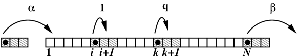
Figure 1: Model for TASEP with extended objects and a local inhomogeneity. System with size $l=3$ particles is shown. Hopping rate in the bulk is $1$. Hopping rate at special site $k$ is $q$. Entrance and exit rates are $\alpha$ and $\beta$, respectively.

2.2 Results for homogeneous TASEP with extended objects

Analytical mean-field calculations and domain-wall arguments, supported by extensive Monte Carlo simulations, indicate that homogeneous TASEP with extended objects has the same three-phase diagram as homogeneous standard TASEP with $l=1$ [7, 8].

For $\alpha\geq\frac{1}{\sqrt{l}+1}$ and $\beta\geq\frac{1}{\sqrt{l}+1}$, the dynamics of the system is determined in the bulk, and we have a maximal-current phase with the stationary current and bulk density given by

$$J=\frac{1}{(\sqrt{l}+1)^{2}},\quad\rho=\frac{\sqrt{l}}{\sqrt{l}+1}.$$ (1)

When the particle entry is the rate-limiting step, which is realized for $\alpha<\frac{1}{\sqrt{l}+1}$ and $\alpha<\beta$, the system is in a low-density stationary phase with the following current and bulk densities:

$$J=\frac{\alpha(1-\alpha)}{1+(l-1)\alpha},\quad\rho=\frac{\alpha l}{1+(l-1)\alpha}.$$ (2)

The conditions $\beta<\frac{1}{\sqrt{l}+1}$ and $\beta<\alpha$ induce a high-density phase, which is governed by the exit dynamics. In this case the current and bulk densities are given by

$$J=\frac{\beta(1-\beta)}{1+(l-1)\beta},\quad\rho=1-\beta.$$ (3)

There are two types of phase transitions in this system. A first-order phase transition, with discontinuous change in density, is observed when $\alpha=\beta$. However, the transitions between low-density (high-density) and maximal-current phases are continuous.

2.3 Approximate solutions of inhomogeneous TASEP with extended objects

For simplicity, let us assume that the size of the system $N$ is a large even number and that the special site with jumping rate $q$ is positioned at $k=N/2$. The exact position of local inhomogeneity is not important as long as it is far away from both boundaries [11, 12].

The special site $k$ breaks the translational symmetry of original homogeneous TASEP. However, it also divides the system of size $N$ into two homogeneous translationally invariant sublattices of size $N/2$. This observation allows us to consider our model with local inhomogeneity as two coupled homogeneous TASEP with extended objects. The sublattices are coupled by a condition that the stationary currents in the left and right subsystems should be the same. As a result, to calculate the properties of TASEP with extended objects and with local inhomogeneity, we can use the known results for homogeneous TASEP. This approach has been used successfully before in different inhomogeneous asymmetric exclusion models [11, 12]. Note that the results of Ref. [11] correspond to our special case $l=1$, i.e., when each particle occupies only one site.

The main assumption of our theoretical method is that TASEP with local inhomogeneity can be viewed as two independent homogeneous TASEP coupled only by the requirement to have the same steady-state currents. Then each of the sublattices may exist in one of three different stationary states, and there are nine possible phases in the overall system. However, since the particle current in the left subsystem should be equal to the current in the right subsystem, it is impossible to have the maximal-current phase in one of the sublattices while the other sublattice is in the low-density or high-density phase. This observation eliminates four possible stationary phases and leaves only low-density/low-density (ld/ld), high-density/high-density (hd/hd), low-density/high-density (ld/hd), high-density/low-density (hd/ld) and maximal-current/maximal-current (mc/mc) stationary phases. In this notation, the first term corresponds to the state of the left sublattice, while the second term describes the right sublattice.

Consider in a more detail the possibility of existence of an ld/hd phase in our system. This phase may exist only when $\alpha\neq\beta$ and

$$\alpha<\frac{1}{\sqrt{l}+1},\quad\beta<\frac{1}{\sqrt{l}+1}.$$ (4)

Then, because the currents in the sublattices are the same,

$$J=\frac{\alpha(1-\alpha)}{1+(l-1)\alpha}=\frac{\beta(1-\beta)}{1+(l-1)\beta},$$ (5)

which yields

$$\beta=\frac{1-\alpha}{1+\alpha(l-1)}.$$ (6)

However, using the condition (4) for $\alpha$ we may conclude that $\beta>\frac{1}{\sqrt{l}+1}$, which violates the condition for existence of the high-density phase on the right sublattice. Thus the ld/hd phase also cannot be realized in our system.

The local inhomogeneity in our model is realized for different values of $q$. When $q>1$ the fast jumping rate is introduced. In this case, the dynamics near the local inhomogeneity will not affect the overall dynamics in the system since crossing the special site $k$ will not be a rate-limiting step. As a result, we have exactly the same phase diagram as for homogeneous TASEP with extended objects with ld/ld, hd/hd and mc/mc phases. The presence of local inhomogeneity will only modify the density profiles near the site $k$.

The more interesting case is $q<1$, when the dynamics near local inhomogeneity may determine the overall behavior of the system. Now consider in more detail the process of a particle crossing from the left sublattice to the right one. The particle first approaches the right sublattice when its left edge is on the site $k-l+1$. Then it makes $l-1$ jumps with rate 1 and one jump with the rate $q$, if these motions are allowed, and the particle transfers completely into the right subsystem. Thus, the effective rate of moving from the left sublattice to the right sublattice is given by

$$q_{eff}=\frac{l}{1/q+(l-1)}=\frac{lq}{1+q(l-1)}.$$ (7)

If the entrance to the left subsystem is the rate-limiting step, then the system will be in the ld/ld phase with the particle current and bulk density given in (2). This situation is realized for $\alpha$ less than some $\alpha^{*}$. Similarly, when the exit from the right subsystem determines the overall dynamics, the hd/hd phase exists with the particle current and bulk density given in (3), again for $\beta<\beta^{*}$. Parameters $\alpha^{*}$ and $\beta^{*}$ will be calculated explicitly below.

When the transition from the left sublattice to the right sublattice becomes the rate-limiting step, the hd/ld phase is realized in our system. The parameters for existence of this phase can be found from the condition that the current through left sublattice is equal to the current through the right sublattice and equal to the current passing through the local inhomogeneity. Following the expressions (2) and (3), the stationary current and bulk density in the left sublattice are given by

$$J_{left}=\frac{\beta_{eff}(1-\beta_{eff})}{1+\beta_{eff}(l-1)},\quad\rho_{left}=1-\beta_{eff},$$ (8)

while in the right sublattice,

$$J_{right}=\frac{\alpha_{eff}(1-\alpha_{eff})}{1+\alpha_{eff}(l-1)},\quad\rho_{right}=\frac{l\alpha_{eff}}{1+\alpha_{eff}(l-1)},$$ (9)

where $\beta_{eff}$ is the effective rate to exit from the left sublattice and $\alpha_{eff}$ is the effective rate to enter the right sublattice. The current passing through the local inhomogeneity can be written as

$$J_{0}=q_{eff}\frac{\rho_{left}}{l}\frac{(1-\rho_{right})}{(1-\rho_{right}+\rho_{right}/l)}.$$ (10)

This expression can be understood as follows. The parameter $q_{eff}$, which is given explicitly in (7), is an effective rate of crossing the local inhomogeneity. The factor $\frac{\rho_{left}}{l}$ is the probability to find a particle at site $k-l+1$, i.e., the particle is crossing from the left sublattice to the right sublattice. Finally, $\frac{(1-\rho_{right})}{(1-\rho_{right}+\rho_{right}/l)}$ is the conditional probability for the corresponding sites in the right sublattice to be empty (as in [8]). The condition of stationary state implies that $J_{left}=J_{0}=J_{right}$, which yields

$$\rho_{right} = \frac{\rho_{left}-(1-q_{eff})[l-\rho_{left}(l-1)]}{1-(1-q_{eff})[l-\rho_{left}(l-1)]},$$

$$\rho_{right} = q_{eff}\rho_{left}.$$ (11)

Solving these equations leads to expressions for the densities in the right and left sublattices:

$$\rho_{left} = \frac{(1+q_{eff})l}{2q_{eff}(l-1)}\left[1-\sqrt{1-\frac{4q_{eff}(l-1)}{l(1+q_{eff})^{2}}}\right],$$

$$\rho_{right} = q_{eff}\rho_{left}.$$ (12)

The explicit formula for the current can be found from (10). This phase can only exist when $\alpha>\beta_{eff}$ and $\beta>\alpha_{eff}$, and using (8), (9) and (2.3) we obtain that hd/ld phase is stable for $\alpha>\alpha^{*}$ and $\beta>\beta^{*}$, where

$$\alpha^{*}=\beta^{*}=1-\frac{(1+q_{eff})l}{2q_{eff}(l-1)}\left[1-\sqrt{1-\frac{4q_{eff}(l-1)}{l(1+q_{eff})^{2}}}\right].$$ (13)

Our theoretical results can be easily checked in some special limiting cases. For $q=q_{eff}=1$, and $\alpha>\alpha^{*},\beta>\beta^{*}$, we obtain that the bulk densities at the left and right sublattices are the same and equal to $\rho_{left}=\rho_{right}=\sqrt{l}/(\sqrt{l}+1)$, i.e., the system is in the maximal-current phase, in agreement with known results [7, 8]. In the limit of $q\rightarrow 0$, the effective rate of crossing the local inhomogeneity is also very small, $q_{eff}\approx lq$. In this limit the bulk densities reduce to $\rho_{left}\approx 1-q$ and $\rho_{right}\approx lq$, in agreement with intuitive expectations. These results can be understood as follows. Particles will move into the right sublattice with a rate of $q$, so that the spacing between the particles will be about $1/q$ (distance traveled before the next particle comes into the sublattice), giving a coverage density of $lq$. Now consider the left sublattice. It will be nearly full, so consider the backwards current of holes moving through the slow site. Holes will enter the left sublattice at a rate $q$, so the hole density will be $q$. Hence the coverage density in the left sublattice will be $1-q$. Another interesting limit is $l\gg 1$, which corresponds to the case of very large particles. In this limit we obtain $J\approx 1/l$, as was found before for the homogeneous model [7].

It is interesting to note that our theory predicts a “mixed” nature of phase transitions from hd/ld to ld/ld or hd/hd phases. At one sublattice the transition will be continuous, while at the other sublattice there is a jump in density, which corresponds to a first-order phase transition.

3 Monte Carlo simulations and discussions

Our theoretical approach gives correct results in limiting cases. However, to check the overall validity of our approximate theory we performed Monte Carlo computer simulations.

Monte Carlo simulations were implemented similarly to those in [8]. Random sequential updating was used. Suppose that at some time the lattice contains $M$ particles. Then in the next Monte Carlo step (MCS), $M+1$ particles are chosen at random, in sequence, to attempt moves. They are selected from a pool containing the $M$ particles on the lattice plus a free particle that can enter the system with probability $\alpha$ if the first $l$ sites are empty. Particles on lattice site $k$ advance with probability $q$ if site $k+l$ is empty. Particles on site $N$ leave the system with probability $\beta$. All other particles advance if they have room to move. Simulations were begun with an empty lattice and run until steady state was reached. For particles with $l=12$, the size studied in greatest detail, the system size was $N=2500$, and $3\times 10^{5}$ MCS were allowed to reach steady state. For other particle sizes, the system was run for at least $100N$ MCS to reach steady state. After steady state was attained, systems were simulated for an additional $1.5\times 10^{6}$ Monte Carlo steps, during which the current leaving the system was recorded constantly, and the particle density at each lattice site was sampled every 100 MCS. Continuous time Monte Carlo [13] was used to reduce the computation time required.

The phase diagram was determined in detail from simulations for $l=12$, $q=0.2$, and $N=2500$ (see Fig. 2). From the theory, we expected the ld/ld phase to occur for $\alpha<\alpha^{*}=0.1338$, $\alpha<\beta$, the hd/hd phase to occur for $\beta<\beta^{*}=0.1338$, $\beta<\alpha$, and the hd/ld phase to occur for $\alpha,\beta>0.1338$. Simulations were consistent with these expectations. Sample density profiles from each phase are shown in Fig. 3. The theoretical predictions for currents and bulk densities in each half of the system also matched the simulations to within $1\%$ (see Fig 4).

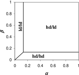
Figure 2: Phase diagram for $l=12$, $q=0.2$. Locations of phase transitions were determined via simulations to within $0.02$ and were in agreement with predictions.

Figure 3: Sample density profiles from simulations for the ld/ld phase (top, $\alpha=0.05,\beta=0.5$), the hd/ld phase (middle, $\alpha=0.5,\beta=0.5$), and the hd/hd phase (bottom, $\alpha=0.5,\beta=0.05$). All cases have $q=0.2$, $l=12$, $N=2500$.

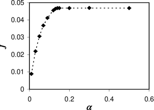
[a] [b]

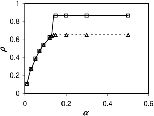
Figure 4: (a) Dependence of current $J$ on $\alpha$. (b) Dependence of bulk densities $\rho_{left}$ (squares, solid curve) and $\rho_{right}$ (triangles, dashed curve) on $\alpha$. Bulk densities were spatial and time averages over regions in which the density profile was approximately constant. $\rho_{left}$ values are omitted near the phase transition because the density profile was approximately linear in the left half of the system. In all cases, symbols are simulation results, and curves are predicted values. Results are for $\beta=0.5,q=0.2,l=12,N=2500$. Error bars, determined from standard deviations for simulations run in triplicate, are smaller than size of symbols.

The phase transitions were identified as follows. Near the transition between the hd/hd phase and the hd/ld phase, in the right half of the system, $\alpha_{eff}\approx\beta$. This situation is expected to produce shock waves in the right half of the system (see [8]). We detected these shock waves in simulations by observing the approximately linear density profile that they produce in the right half of the system. An example of a density profile for the hd/hd to hd/ld transition is shown in Fig. 5. Similarly, the left half of the system exhibits an approximately linear density profile near the ld/ld to hd/ld transition, and both halves of the system have approximately linear density profiles near the ld/ld to hd/hd transition. Visual inspection of the density profiles allows the transition lines to be localized to within about $0.02$ units. Other techniques would be required to find the transition lines more precisely. For example, we could determine the boundaries of the hd/ld phase by measuring the current as a function of $\alpha$ or $\beta$ and determining at which $\alpha$ or $\beta$ the current saturates.

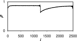
Figure 5: Sample density profile near the transition from the hd/hd to the hd/ld phase. Parameters are $\alpha=0.2,q=0.2,\beta=0.13,l=12,N=2500$. The transition is expected to occur at $\beta=0.1338$. Because of the proximity to the phase transition, the density profile is approximately linear in the right half of the system.

Simulations were conducted in each phase for other values of $l$ ($l=2,5,20$) to confirm the theoretical predictions. System sizes $N$ were always at least $200l$, in keeping with the assumption of large $N$. The theoretical predictions for the current and bulk densities were generally more accurate for larger particles. The greatest discrepancies between theory and simulations were seen for $l=2$ in the hd/ld phase, but observed discrepancies were always less than $10\%$. These results show that our approximate theory becomes more exact for larger-size particles. This is because the particle-particle correlations decrease with increasing $l$. Consider a lattice consisting of $N=nl$ sites with $M$ particles (each of size $l$). If we assume that particles are uniformly distributed, we can easily estimate the average number of empty sites $x_{l}$ between two neighboring particles: $x_{l}=\frac{nl-Ml}{M}=lx_{1}$. Thus the number of empty sites between the particles grows linearly with the particle size $l$. As result, particles correlate to lesser degree with each other, and our theoretical mean-field approach becomes more accurate. Similar conclusions have been reached in Ref. [7].

The phase diagram and phase transitions in TASEP with extended objects and with a local inhomogeneity can also be easily explained with the help of the domain-wall theory [9]. As we discussed above, the introduction of local inhomogeneity divides the system into the two homogeneous sublattices, and the phase behavior in each sublattice is determined by the dynamics of domain walls. Thus there are always two domain walls present in the system. In the hd/ld phase at stationary state the domain walls are localized near the entrance and the exit of the system, while in ld/ld stationary phase the domain walls can be found diffusing near the local inhomogeneity and the exit. Similarly, in hd/hd stationary phase the domain walls are near the entrance and the local inhomogeneity. The phase transitions can be associated with the change of position of domain walls. For example, the transition from ld/ld phase to hd/ld phase (when $q<1$) is the consequence of the motion of the domain wall from the position of local inhomogeneity to the entrance, while the second domain wall stays at the exit. This observation also explains the “mixed” nature of this phase transition.

4 Summary and conclusions

We investigated the effect of inhomogeneity in totally asymmetric simple exclusion processes with particles of arbitrary size. Specifically, the simple model with one inhomogeneous jumping rate in the middle of the system was considered. The model was solved using a simple approximate method. Our analytical approach was based on two assumptions. The first one is the fact that the local inhomogeneity divides the system into the two coupled homogeneous systems, for which very precise mean-field solutions already exist. In the second approximation we assumed that the dynamics of particles in each sublattice is independent, i.e., we neglected the correlations between the particles in the two coupled subsystems. Using these assumptions, we calculated explicitly the phase diagrams, bulk densities, and stationary currents.

Our theoretical results indicate that for a fast jumping rate ($q\geq 1$), the phase diagrams, currents and bulk densities do not change as compared with homogeneous TASEP with extended objects. However, for the slow jumping rate, the situation is different. As in the homogeneous TASEP, three stationary phases are found, although phase boundaries, stationary currents and bulk densities change significantly. Our theoretical predictions are well supported by extensive Monte Carlo simulations. Some small deviations between the analytical theory and computer simulations are due to the neglect of correlations near local inhomogeneity in our theoretical approach. However, the precision of our theoretical predictions increases with the size of the particles. The microscopic nature of phase diagram was analyzed using phenomenological domain-wall theory.

Although we considered only totally asymmetric exclusion processes, our theoretical arguments can be easily extended to more general partially asymmetric exclusion processes where particles can hop in both directions. However, the important parameter of effective crossing rate from the left sublattice to the right should be calculated using more general expressions, $q_{eff}=l/\tau$, where $\tau$ is mean first-passage time for the particle to move to the right sublattice. It can be calculated using standard procedures [14].

References

References

- [1] Derrida B 1998 Phys. Rep 301 65
- [2] Schütz G M 2000 Integrable stochastic many-body systems Phase Transitions and Critical Phenomena vol 19, ed Domb and Lebowitz (London: Academic)
- [3] MacDonald J T, Gibbs J H and Pipkin A C 1968 Biopolymers 6 1
- [4] Schütz G M 1999 Europhys. Lett 48 623
- [5] Chou T 1998 Phys. Rev. Lett. 80 85
- [6] Popkov V, Santen L, Schadschneider A and Schütz G M 2001 J. Phys. A: Math. Gen. 34 L45
- [7] Lakatos G and Chou T 2003 J. Phys. A: Math. Gen. 36 2027
- [8] Shaw L B, Zia R K P and Lee K H 2003 Phys. Rev. E 68 021910
- [9] Kolomeisky A B, Schütz G M, Kolomeisky E B and Straley J P 1998 J. Phys. A: Math. Gen. 31 6911
- [10] Stryer L, 1995 Biochemistry (W.H. Freeman, New York)
- [11] Kolomeisky A B 1998 J. Phys. A: Math. Gen. 31 1153
- [12] Mirin N and Kolomeisky A B 2003 J. Stat. Phys. 110 811
- [13] Bortz A, Kalos M, and Lebowitz J 1975 J͡. Comp. Phys. 17 10
- [14] van Kampen N G, 1992 Stochastic Processes in Physics and Chemistry (Amsterdam: Elsevier) Chap XII.