SU(2) Non-Abelian Holonomy and Dissipationless Spin Current in Semiconductors

Abstract

Following our previous work [S. Murakami, N. Nagaosa, S. C. Zhang, Science 301, 1348 (2003)] on the dissipationless quantum spin current, we present an exact quantum mechanical calculation of this novel effect based on the linear response theory and the Kubo formula. We show that it is possible to define an exactly conserved spin current, even in the presence of the spin-orbit coupling in the Luttinger Hamiltonian of p-type semiconductors. The light- and the heavy-hole bands form two Kramers doublets, and an $SU(2)$ non-abelian gauge field acts naturally on each of the doublets. This quantum holonomy gives rise to a monopole structure in momentum space, whose curvature tensor directly leads to the novel dissipationless spin Hall effect, i.e., a transverse spin current is generated by an electric field. The result obtained in the current work gives a quantum correction to the spin current obtained in the previous semiclassical approximation.

I Introduction

Spintronics, the science and technology of manipulating the spin of the electron for building integrated information processing and storage devices, showed great promise wolf2001 . Spintronics devices also promises to access the intrinsic quantum regime of transport, paving the path towards quantum computing. However, many challenges remain in this exciting quest. Among them, purely electric and dissipationless manipulation of the electron spin and its quantum transport is one of the most important goals of quantum spintronics.

In our previous work murakami2003 , we discovered a basic law of spintronics, which relates the spin current and the electric field by the response equation

$$j_{j}^{i}=\sigma_{s}\epsilon_{ijk}E_{k}$$ (1)

where $j_{j}^{i}$ is the current of the $i$-th component of the spin along the direction $j$ and $\epsilon_{ijk}$ is the totally antisymmetric tensor in three dimensions. Sinova et al. sinova2003 found a similar effect in the two-dimensional n-type semiconductors with Rashba coupling. This law is similar to Ohm’s law in electronics, and the spin conductivity $\sigma_{s}$ has the dimension of the electric charge $e$ divided by the scale of length. However, unlike the Ohm’s law, this fundamental response equation describes a purely topological and dissipationless spin current. It is important to note here that the spin current is even under the time-reversal operation ${\cal T}$. When the direction of the arrow of time is reversed, both the direction of the current and the spin are reversed and the spin current remains unchanged. Since both the spin current and the electric field in Eq. (1) are even under time reversal ${\cal T}$, the transport coefficient $\sigma_{s}$ is called “reactive” and can be purely non-dissipative. This is in sharp contrast to the Ohm’s law

$$j_{i}=\sigma E_{i}$$ (2)

relating the charge current $j_{i}$ to the electric field. In this case, the charge current $j_{i}$ changes sign under time-reversal ${\cal T}$, while the electric field is even under ${\cal T}$. Since the Ohm’s law relates quantities of different symmetries under time reversal ${\cal T}$, the charge conductivity $\sigma$ breaks the time-reveral symmetry and describes the inevitable joule heating and dissipation. Quantum Hall current, which is transverse to the electric field and dissipationless, has the feature similar to Eq. (1), but the time-reversal symmetry is compensated by the external magnetic field. Dissipationless current without time-reversal symmetry breaking is extremely important and fundamental in solid-state physics, the most celebrated example of which is the superconducting current. It is described by the London equation,

$$j_{i}=\frac{\rho_{s}e^{2}}{mc}A_{i}\ \ ,\ \ E_{i}=-\frac{1}{c}\frac{\partial A_{i}}{\partial t}$$ (3)

where the current $j_{i}$ is related to the vector potential $A_{i}$ instead of the electric field. In the London equation, both $j_{i}$ and $A_{i}$ are odd under time reversal ${\cal T}$, therefore, the transport coefficient $\rho_{s}$, also called the superfluid density, describes the reversible and dissipationless flow of the supercurrent.

In summary, the dissipationless spin current discovered in Ref. murakami2003, shares some basic features with the superconducting current and the quantum Hall edge current, in the sense that, 1) the spin Hall conductivity $\sigma_{s}$ is a dissipationless or reactive transport coefficient, even under the time-reversal operation ${\cal T}$; 2) the spin Hall conductivity $\sigma_{s}$ can be expressed as an integral over all states below the fermi energy, not only over states in the vicinity of the fermi energy as in most dissipative transport coefficients. Furthermore, just like the case of the quantum Hall effectthouless1982 ; sundaram1999 , the contribution of each state to the spin Hall conductivity $\sigma_{s}$ can be expressed entirely in terms of the curvature of a gauge field in momentum space, which in our case is non-abelian. The dissipationless spin current is induced by the electric field through the spin-orbit coupling, whose characteristic energy scale exceeds the room temperature in many semiconducting materials.

Electronic structure of semiconductors with diamond structure (e.g. Si, Ge) and zincblende structure (e.g. GaAs, InSb) are well understood in terms of the ${\bf k}\cdot{\bf p}$ perturbation theory. The top of the valence bands are at ${\bf k}={0}$, i.e., $\Gamma$-point. They consist of the three p-orbitals $p_{x},p_{y},p_{z}$ with spin up and down. In the presence of the relativistic spin-orbit coupling, these 6 states are split into four-fold degenerate $S=3/2$ states and two-fold degenerate $S=1/2$ state. Here $S$ denotes the total angular momentum of the atomic orbital, obtained through the coupling of the orbital angular momentum $L$ and the spin angular momentum $s$. The second order perturbation in the ${\bf k}\cdot{\bf p}$ results in the effective Hamiltonian near ${\bf k}={0}$, which is called Luttinger Hamiltonianluttinger1956 :

$$H_{0}=\sum_{\mathbf{k}}c_{\mu,\mathbf{k}}^{\dagger}H_{\mu\nu}(\mathbf{k})c_{\nu,\mathbf{k}}$$

$$H_{\mu\nu}(\mathbf{k})=\frac{1}{2m}\left((\gamma_{1}+\frac{5}{2}\gamma_{2})k^{2}-2\gamma_{2}(\mathbf{k}\cdot\mathbf{S})^{2}\right)_{\mu\nu}$$ (4)

where $\mathbf{k}=(k_{x},\ k_{y},\ k_{z})$, $\mathbf{S}=(S^{x},\ S^{y},\ S^{z})$, and $k=|\mathbf{k}|$. The explicit form of the matrices $S^{i}$ $(i=1,2,3)$ is given in Appendix A. For simplicity, we have put $\gamma_{2}=\gamma_{3}$ in the original Luttinger Hamiltonian; most of subsequent discussions are also applicable to more general cases with $\gamma_{2}\neq\gamma_{3}$.

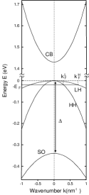
Figure 1: Schematic picture of the band structure of GaAs near $\mathbf{k}=0$. CB means the conduction band, HH the heavy-hole band, LH the light-hole band, and SO the split-off band, respectively. When the small inversion symmetry breaking is neglected, all of them are doubly degenerate. The Fermi energy shown in the figure corresponds to the hole density $\sim 10^{19}\text{cm}^{-3}$. The splitting $\Delta=0.34$eV at $\mathbf{k}=0$ between the LH,HH and SO bands are due to the spin-orbit interaction. The HH and LH bands are degenerate at $\mathbf{k}=0$, giving rise to a monopole in the gauge field as discussed in Section III

On the other hand, the conduction bands are made out of the s-orbital and hence doubly degenerate. When we neglect a small effect due to broken inversion symmetry, this degeneracy is not lifted due to the Kramers theorem. Therefore the effect of the spin-orbit interaction is small in the conduction band, although the Rashba effect rashba1960 ; bychkov1984 ; nitta1997 ; datta1990 is induced by the electric field near e.g. the interface structure. The spin Hall current in the Rashba system has recently been discussed by Sinova et al. sinova2003 . These authors showed that dissipationless and intrinsic spin Hall current can take an universal value in this system. The position of the conduction band minima depends on the material. For example, they are located at general points along the axis between the $\Gamma$- and the $X$-points in Si, while they at at the $L$-points in Ge. We will focus on the valence bands below because of the intrinsically strong spin-orbit interaction.

Although the band structure of semiconductors with spin-orbit coupling has been understood for many years, only recently has it been recognized that the gauge field and its curvature in the momentum space made out of the Bloch wavefunction play important roles in the transport properties of electrons in solids. The gauge field is defined in terms of the Bloch state $|n\mathbf{k}\rangle$ as

$$A_{ni}(\mathbf{k})=-i\left\langle n\mathbf{k}\left|\frac{\partial}{\partial k_{i}}\right|n\mathbf{k}\right\rangle,$$ (5)

where $n$ is a band index. It represents the inner product of the two Bloch wavefunctions infinitesimally separated in $\mathbf{k}$-space. This gauge field $A_{ni}(\mathbf{k})$ describes topological structure of Bloch wavefunctions in the momentum space thouless1982 ; sundaram1999 , and plays an important role in transport properties matl1998 ; ye1999 ; chun2000 ; ohgushi2000 ; taguchi2001 ; jungwirth2002 ; taguchi2003 ; fang2003 ; yasui2003 and in magnetic superconductors murakami2003b . In particular, this gauge field is related to the transverse conductivity $\sigma_{xy}$ as

$$\sigma_{xy}=-\frac{e^{2}}{h}\sum_{n,\mathbf{k}}n_{F}(\epsilon_{n}(\mathbf{k}))B_{nz}(\mathbf{k}),$$ (6)

where $B_{nz}(\mathbf{k})=F_{n,xy}(\mathbf{k})=\frac{\partial A_{ny}(\mathbf{k})}{\partial k_{x}}-\frac{\partial A_{nx}(\mathbf{k})}{\partial k_{y}}$ is the $z$-component of the field strength made from $A_{ni}(\mathbf{k})$, and $n_{F}(\epsilon_{n}(\mathbf{k}))$ is the Fermi distribution of fr the $n$-th band with energy $\epsilon_{n}(\mathbf{k})$. This formula thouless1982 ; sundaram1999 is the foundation of the integer quantum Hall effect (QHE), and further applied to the anomalous Hall effect (AHE) in ferromagnetic metals matl1998 ; ye1999 ; chun2000 ; ohgushi2000 ; taguchi2001 ; jungwirth2002 ; taguchi2003 ; fang2003 ; yasui2003 . Especially in the magnetic semiconductors (Ga,Mn)As ohno1998 , the calculation jungwirth2002 by the formula Eq. (3) well explains the experimental results quantitatively, giving some credit that the AHE is mostly of intrinsic origin rather than extrinsic origins, e.g., skew scattering and/or side-jump mechanism. However in the presence of the time-reversal symmetry, the d.c. transverse conductivity $\sigma_{xy}$ vanishes, and the topological structure of the Bloch wavefunctions has not been systematically studied in the context of transport theory. As we will show below, an even more beautiful and nontrivial quantum topological structure is hidden in the valence-band structure in the paramagnetic state, which is analogous to the fermionic quasi-particles in the SO(5) theorydemler1999 . This is also motivated by the recent work by one of the present authors on the generalization of the quantum Hall effect into four dimensions in terms of the SO(5) symmetryzhang2001 . In this paper, we shall show that the SO(5) group structure of the $S=3/2$ Bloch states provides a natural description of the non-abelian $SU(2)$ holonomy and its curvature in momentum space. This gauge structure underlies the dissipationless, topological spin current in hole-doped semiconductors.

In the presence of the spin-orbit interaction, the conventionally defined total spin operator is not conserved, and it is nontrivial to define the spin current in this case. Our formalism resolves this issue by discovering conserved quantities in the Luttinger Hamiltonian (4) and by defining associated conserved spin currents. These quantities have clear physical and geometric meanings. The exact quantum calculation of the conserved spin Hall conductivity $\sigma_{s}$ is performed in terms of the Kubo formula, and the results can be expressed entirely in terms of the non-abelian gauge curvature in momentum space. Our fully quantum mechanical results identify the quantum correction to the previous semiclassical resultmurakami2003 in terms of the wave-packet formalism.

The plan of this paper is as follows. In section II, we reformulate the Luttinger Hamiltonian in terms of the SO(5) algebra and give the definition of the conserved spin current. Based on this definition, the calculation of the spin Hall conductivity in terms of Kubo formula is presented in section III, where the geometrical meaning is stressed, and the comparison with the previous semiclassical result is given. Section IV is devoted to conclusions. Throughout the paper, we take the unit $\hbar=1$, $e=1$.

II Definition of the spin current

The Luttinger Hamiltonian (4) has two eigenvalues:

$$E_{L}(k)=\frac{\gamma_{1}+2\gamma_{2}}{2m}k^{2}\ \ ,\ \ E_{H}(k)=\frac{\gamma_{1}-2\gamma_{2}}{2m}k^{2}$$ (7)

corresponding to the light-hole (LH) and the heavy-hole (HH) bands. Each eigenvalues are doubly degenerate, due to the Kramers theorem based on the time-reversal symmetry. For a fixed value of $\mathbf{k}$, let $P^{L}(\mathbf{k})$ denote a projection onto the two-dimensional subspace of states of the LH band. We also define $P^{H}(\mathbf{k})$ similarly. These operators are written as

$$P^{L}=\frac{9}{8}-\frac{1}{2k^{2}}(\mathbf{k}\cdot\mathbf{S})^{2}\ \ ,\ \ P^{H}=1-P^{L}$$ (8)

They obviously satisfy

$$P^{L}P^{H}=0=P^{H}P^{L},\ \ (P^{L})^{2}=P^{L},\ \ (P^{H})^{2}=P^{H}$$ (9)

In terms of these projectors, the Luttinger Hamiltonian can be expressed as

$$H=\sum_{\mathbf{k}}(E_{H}(\mathbf{k})P^{H}(\mathbf{k})+E_{L}(\mathbf{k})P^{L}(\mathbf{k})).$$ (10)

From this projector form of the Hamiltonian, we see that the LH and the HH bands are each two-fold degenerate, and there is an SU(2) rotation symmetry acting on each band. Combining the LH and the HH bands, there is an SO(4)$=$SU(2)$\times$SU(2) symmetry at every $\mathbf{k}$ point. In this section, we shall develop the mathematical framework in which this SO(4) symmetry is made manifest, and this symmetry is used to define the conserved spin current. Since $P^{H}$ and $P^{L}$ depend on $\mathbf{k}$, the quantization axis for each SU(2) varies as a function of $\mathbf{k}$. When $\mathbf{k}$ is adiabatically changed along a closed circuit, the fermionic wave function in general does not return to itself; in fact, the final wave function is related to the starting wave function by an SU(2) transformation within each band. Therefore, this problem is a natural generalization of Berry’s U(1) phaseberry1984 to the case of SU(2) holonomywilczek1984 ; avron1988 ; zee1988 ; mathur1991 ; shankar1994 ; arovas1998 ; demler1999 . In particular, Demler and Zhangdemler1999 developed a formalism of the SU(2) non-abelian holonomy in terms of the SO(5) Clifford algebra, which we shall adopt throughout this paper. Upon expanding the $(k_{i}S^{i})^{2}$ term in the Hamiltonian (4), we obtain a product of two quadratic forms, one of the form $\xi_{a}^{ij}k_{i}k_{j}$ and another of the form $\xi_{a}^{ij}S^{i}S^{j}$, where $\xi_{a}^{ij}$ is a symmetric matrix. A 3$\times$3 symmetric matrix can be further decomposed into one trace and five traceless parts. The trace part has the same form as the first term in the Hamiltonian (4), and cancels the $\gamma_{2}$ contribution by construction. The remaining five traceless symmetric ($\xi_{a}^{ij}=\xi_{a}^{ji},\xi_{a}^{ii}=0$) combination of $\xi_{a}^{ij}S^{i}S^{j}$ can be identified with the Clifford algebra of the Dirac $\Gamma$ matrices, with the identification

$$\Gamma^{a}=\xi_{a}^{ij}\{S^{i},S^{j}\}\ ,\ \ \{\Gamma^{a},\Gamma^{b}\}=2\delta_{ab}$$ (11)

The explicit forms of $S^{i},\Gamma^{a}$ and $\xi_{a}^{ij}$ are given in Appendix A. In terms of the $\Gamma$ matrices, the Luttinger Hamiltonian (4) takes the elegant form

$$H(k)=\epsilon(\mathbf{k})+\frac{\gamma_{2}}{m}d_{a}\Gamma^{a},$$ (12)

where

$$\epsilon(\mathbf{k})=\frac{\gamma_{1}}{2m}k^{2},\ d_{a}(\mathbf{k})=-3\xi_{a}^{ij}k_{i}k_{j},$$

$$d_{1}=-\sqrt{3}k_{y}k_{z},\ d_{2}=-\sqrt{3}k_{x}k_{z},\ d_{3}=-\sqrt{3}k_{x}k_{y},$$

$$d_{4}=-\frac{\sqrt{3}}{2}(k_{x}^{2}-k_{y}^{2}),$$

$$d_{5}=-\frac{1}{2}(2k_{z}^{2}-k_{x}^{2}-k_{y}^{2}).$$ (13)

We recognize that the vector components of $d_{a}(\mathbf{k})$ are nothing but the five d-wave combinations in the $\mathbf{k}$ space. The five-dimensional vector $\mathbf{d}$ provides a mapping from the three-dimensional $\mathbf{k}$ space to the five-dimensional $\mathbf{d}$ space (Fig. 2). Since the Luttinger Hamiltonian depends on $\mathbf{k}$ only through $\mathbf{d(k)}$, we can perform all calculations in the 5D $\mathbf{d}$ space, and finally project back onto the 3D $\mathbf{k}$ space. This formalism enables a unified treatment for the anisotropic Luttinger Hamiltonian, and more importantly, reveals the deep connection to the four-dimensional quantum Hall effect (4DQHE) zhang2001 . Here and henceforth we adopt the convention that indices appearing twice are summed over.

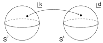
Figure 2: Mapping from the three-dimensional $\mathbf{k}$ vector space to the five-dimensional $\mathbf{d}$ vector space. The gauge structures of the spin current are associated with the magnetic monopoles located at the origins of the $\mathbf{k}$ and $\mathbf{d}$ spaces.

The eigenvalues of (12) are $E_{L}(\mathbf{k})=\epsilon(\mathbf{k})+\frac{\gamma_{2}}{m}d(\mathbf{k})$ and $E_{H}(\mathbf{k})=\epsilon(\mathbf{k})-\frac{\gamma_{2}}{m}d(\mathbf{k})$, where $d(\mathbf{k})=\sqrt{d_{a}d_{a}}=k^{2}$. They are of course the same as (7). In terms of the $\Gamma$ matrices, the projection operators (8) can be expressed as

$$P^{L}=\frac{1}{2}(1+\hat{d}_{a}\Gamma^{a})\ \ ,\ \,P^{H}=\frac{1}{2}(1-\hat{d}_{a}\Gamma^{a}),$$ (14)

where $\hat{d}_{a}=d_{a}/d$. The $\Gamma$ matrices are convenient for subsequent calculations, since a product of any number of $\Gamma$ matrices can be easily reduced to a linear combination of $1$, $\Gamma^{a}$ and $\Gamma^{ab}=\frac{1}{2i}[\Gamma^{a},\Gamma^{b}]$. The five $\Gamma^{a}$ matrices contain the most general quadratic terms of the spin operator $S^{i}$, while the ten $\Gamma^{ab}$ matrices contain both the three spin operators $S^{i}$ and the seven cubic, symmetric and traceless combinations of spin operators of the form $S^{i}S^{j}S^{k}$, as discussed in Appendix A. These ten spin operators are generated under the Heisenberg time evolutions of the single spin operators, and it is natural to group them all into a unified object. For $\gamma_{2}=0$, $\Gamma^{ab}$ commutes with the Hamiltonian and generates an SO(5) symmetry group of the Hamiltonian. (In fact, the Hamiltonian has a higher, SU(4) symmetry in this case). For a given $\mathbf{k}$, a fixed $\mathbf{d}$ vector singles out a particular direction in the five-dimensional $\mathbf{d}$ vector space, and the second term in (12) breaks the SO(5) symmetry to an SO(4) symmetry. This is nothing but SO(4)$=$ SU(2)$\times$SU(2) symmetry which we discussed earlier. In this way, we see that the SO(5) formalism gives an elegant geometric interpretation of the SU(2)$\times$SU(2) symmetry of the LH and the HH bands. It is in fact a subgroup of SO(5) rotation which keeps a fixed $\mathbf{d}$ vector invariant. As we shall see later in the paper, and in Appendix C, the 3D monopole structure in $\mathbf{k}$ space can be best understood in terms of the monopole structure in the 5D $\mathbf{d}$ space.

To find the conserved quantities, let us define the conserved spin density explicitly as

$$\rho^{ab}(\mathbf{p},\mathbf{q})=c_{\mathbf{p}+\frac{\mathbf{q}}{2},\mu}^{\dagger}P_{ab,cd}(\mathbf{p},\mathbf{q})\Gamma_{\mu\nu}^{cd}c_{\mathbf{p}-\frac{\mathbf{q}}{2},\nu},$$ (15)

where $P_{ab,cd}=P_{cd,ab}=-P_{ba,cd}=-P_{ab,dc}$. For the conservation of the spin, we require that $-i\dot{\rho}^{ab}(\mathbf{p},\mathbf{q})=[H,\rho^{ab}(\mathbf{p},\mathbf{q})]$ is proportional to $\mathbf{q}$ for small $|\mathbf{q}|$. This is realized by imposing a condition on $P_{ab,cd}$ as

$$P_{ab,cd}(\mathbf{p},\mathbf{q})\left(d_{c}\left(\mathbf{p}+\frac{\mathbf{q}}{2}\right)+d_{c}\left(\mathbf{p}-\frac{\mathbf{q}}{2}\right)\right)=0$$ (16)

or equivalently,

$$P_{ab,cd}(\mathbf{p},\mathbf{q})\left(d_{a}\left(\mathbf{p}+\frac{\mathbf{q}}{2}\right)+d_{a}\left(\mathbf{p}-\frac{\mathbf{q}}{2}\right)\right)=0.$$ (17)

From these relations it follows that

$$\rho^{ab}(\mathbf{p},\mathbf{q})\left(d_{a}\left(\mathbf{p}+\frac{\mathbf{q}}{2}\right)+d_{a}\left(\mathbf{p}-\frac{\mathbf{q}}{2}\right)\right)=0.$$ (18)

There are five such linear equations, but only four of them are linearly independent because of the antisymmetry of $\rho^{ab}$. Originally, $\rho^{ab}$ has 10 degrees of freedom, subtracting 4 constraints gives the remaining 6 degrees of freedom, exactly the same as the number of generators in SO(4) algebra. Therefore, the projection operator $P_{ab,cd}$ projects the full SO(5) symmetry generators into the SO(4) subspace which is orthogonal to a given direction of $\mathbf{d}$.

In the limit $\mathbf{q}=0$, (17) is satisfied by

$$P_{ab,cd}=\frac{1}{2}\left(\delta_{ac}\delta_{bd}-\delta_{ad}\delta_{bc}+\delta_{ad}\hat{d}_{b}\hat{d}_{c}\right.$$

$$\ \ \ -\left.\delta_{bd}\hat{d}_{a}\hat{d}_{c}-\delta_{ac}\hat{d}_{b}\hat{d}_{d}+\delta_{bc}\hat{d}_{a}\hat{d}_{d}\right).$$ (19)

It satisfies $P_{ab,cd}P_{cd,ef}=P_{ab,ef}$, implying that it is properly normalized as a projection. It is interesting to note that $P_{ab,cd}$ can also be expressed as

$$P_{ab,cd}=f_{aba^{\prime}b^{\prime}}f_{a^{\prime}b^{\prime}cd},\ f_{abcd}=\frac{1}{2}\epsilon_{abcde}\hat{d}_{e}.$$ (20)

Inserting (19) into the spin density (15), we obtain

$$\rho^{ab}=\sum_{\mathbf{k}}c^{\dagger}_{\mathbf{k}\mu}P_{ab,cd}(\mathbf{k})(\Gamma^{cd})_{\mu\nu}c_{\mathbf{k}\nu}$$

$$\ \ \ =\sum_{\mathbf{k}}c^{\dagger}_{\mathbf{k}\mu}\left(\Gamma^{ab}-\frac{i}{2}[\hat{d}_{a}\Gamma^{b}-\hat{d}_{b}\Gamma^{a},\hat{d}_{f}\Gamma^{f}]\right)_{\mu\nu}c_{\mathbf{k}\nu}.\ \ \$$ (21)

Because $[\Gamma^{ab},d_{e}\Gamma^{e}]=2i(d_{a}\Gamma^{b}-d_{b}\Gamma^{a})$, we get

$$\rho^{ab}=\sum_{\mathbf{k}}c^{\dagger}_{\mathbf{k}\mu}\left(\Gamma^{ab}-\frac{1}{4}[[\Gamma^{ab},\hat{d}_{e}\Gamma^{e}],\hat{d}_{f}\Gamma^{f}]\right)_{\mu\nu}c_{\mathbf{k}\nu}$$

$$\ \ =\sum_{\mathbf{k}}c^{\dagger}_{\mathbf{k}\mu}\left(P^{L}\Gamma^{ab}P^{L}+P^{H}\Gamma^{ab}P^{H}\right)_{\mu\nu}c_{\mathbf{k}\nu}.$$ (22)

Thus it corresponds to projecting out the inter-band matrix elements of $\Gamma^{ab}$. The conservation of $\rho^{ab}$ becomes manifest in (22), because the Hamiltonian is diagonal in each subspace, i.e. the LH or the HH band.

The equation of continuity determines the uniform spin current to be

$$J_{i}^{ab}=\frac{1}{2}\sum_{\mathbf{k},\mu,\nu}c_{\mathbf{k}\mu}^{\dagger}\left\{\frac{\partial H}{\partial k_{i}},\ P_{ab,cd}\Gamma^{cd}\right\}_{\mu\nu}c_{\mathbf{k}\nu}$$

$$\ \ =\frac{1}{2}\sum_{\mathbf{k},\mu,\nu}c_{\mathbf{k}\mu}^{\dagger}\left\{\frac{\partial\epsilon}{\partial k_{i}}+\frac{\gamma_{2}}{m}\frac{\partial d_{f}}{\partial k_{i}}\Gamma^{f},\right.$$

$$\makebox[56.9055pt]{}\left.P^{L}\Gamma^{ab}P^{L}+P^{H}\Gamma^{ab}P^{H}\right\}_{\mu\nu}c_{\mathbf{k}\nu}.$$ (23)

To connect this spin current with the physical spin current in Ref. murakami2003, , we define a tensor $\eta_{ab}^{i}$ by $S^{i}=\eta_{ab}^{i}\Gamma^{ab}=\frac{1}{2i}\eta_{ab}^{i}[\Gamma^{a},\Gamma^{b}].$ Explicit forms and properties of $\eta_{ab}^{i}$ are summarized in Appendix A. By contracting with $\frac{1}{3}\eta^{k}_{ab}$, the conserved spin takes the form

$$S^{l}_{\text{(c)}}=\frac{1}{3}\eta^{l}_{ab}\rho^{ab}$$

$$\ \ \ =\frac{1}{3}\sum_{\mathbf{k}}c_{\mathbf{k}\mu}^{\dagger}\left(P^{L}S^{l}P^{L}+P^{H}S^{l}P^{H}\right)_{\mu\nu}c_{\mathbf{k}\nu}.$$ (24)

The subscript _(c) denotes the fact that this spin current is conserved. Here, we inserted a factor of $\frac{1}{3}$, because in the LH and HH bands (i.e. $S=3/2$ subspace), the expectation value of the spin angular momentum is one-third of that of the total angular momentum $S^{k}$. Thus, Eq. (24) corresponds to neglecting interband matrix elements of the spin angular momentum. In a matrix form, the corresponding conserved spin current is

$$J^{l}_{i\text{(c)}}=\frac{1}{3}\cdot\frac{1}{2}\left\{\frac{\partial H}{\partial k_{i}},\ P^{L}S^{l}P^{L}+P^{H}S^{l}P^{H}\right\}.$$ (25)

III Kubo formula calculation of the spin current

III.1 Difficulties with the conventional definition of the non-conserved spin current

In order to calculate the spin current response based on Kubo formula, we should first define the “spin current operator”. The conventional definition of the spin current, with spin along the $l$ axis flowing along the $i$ axis, is given by

$$J_{i}^{l}=\frac{1}{3}\cdot\frac{1}{2}\left\{\frac{\partial H}{\partial k_{i}},\ S^{l}\right\}.$$ (26)

Because the spin $S^{l}$ is not conserved, $J_{i}^{l}$ does not satisfy the equation of continuity without any source term. Before presenting the full calculation based on the conserved spin current discussed in the previous section, we first calculate the linear response of this non-conserved spin current to the applied electric field and then comment on its difficulties. The Kubo formula gives

$$Q_{ij}^{l}(i\nu_{m})=-\frac{1}{V}\int_{0}^{\beta}\langle\hat{T}J_{i}^{l}(u){J}_{j}\rangle e^{i\nu_{m}u}du$$

$$\ \ \ =\frac{1}{V\beta}\sum_{k,n}\text{tr}\left(J_{i}^{l}G(\mathbf{k},i(\omega_{n}+\nu_{m}))J_{j}G(\mathbf{k},i\omega_{n})\right),\ \$$ (27)

where $\nu_{m}=2\pi m/\beta$ ($m$: integer), $\omega_{n}=(2n+1)\pi/\beta$ ($n$: integer), $\beta=1/k_{B}T$, $\hat{T}$ in (27) represents the time-ordering,

$$J_{j}=\sum_{\mathbf{k},\mu,\nu}c_{\mathbf{k}\mu}^{\dagger}\left(\frac{\partial\epsilon}{\partial k_{j}}+\sum_{h}\frac{\partial d_{h}}{\partial k_{j}}\Gamma^{h}\right)_{\mu\nu}c_{\mathbf{k}\nu},$$ (28)

and $G(\mathbf{k},i\omega_{n})$ is the Matsubara Green’s function, given in (108).

In the clean case, the summation over $\omega_{n}$ can be calculated by a contour integral. In the trace operation in the above equation, only the terms of products of four or five $\Gamma$ matrices are nonzero, and the result is

$$Q_{ij}^{l}(\omega+i\delta)=\frac{4i\omega}{V}\sum_{\mathbf{k}}\frac{n_{F}(\epsilon_{L})-n_{F}(\epsilon_{H})}{d(\omega^{2}-4\gamma_{2}^{2}d^{2}/m^{2})}$$

$$\ \ \cdot\left(\frac{\gamma_{2}}{m}\right)^{2}\left(\frac{\gamma_{1}}{2\gamma_{2}}\epsilon_{ljk}k^{2}k_{i}k_{k}-\epsilon_{ijk}k^{2}k_{k}k_{l}\right).$$ (29)

where $\epsilon_{L}(\mathbf{k})=E_{L}(\mathbf{k})-\mu$ and $\epsilon_{H}(\mathbf{k})=E_{H}(\mathbf{k})-\mu$ are one-particle energies for the two bands, measured form the chemical potential $\mu$.

Therefore, in the static limit the linear response is given by

$$\sigma_{ij}^{l}=\lim_{\omega\rightarrow 0}\frac{Q_{ij}^{l}(\omega)}{-i\omega}$$

$$\ \ =\frac{1}{3V}\sum_{\mathbf{k}}\frac{n_{F}(\epsilon_{L})-n_{F}(\epsilon_{H})}{k^{2}}\epsilon_{lji}\left(\frac{\gamma_{1}}{2\gamma_{2}}+1\right)$$

$$\ \ =\frac{1}{6\pi^{2}}\epsilon_{ijl}(k_{F}^{H}-k_{F}^{L})\left(\frac{\gamma_{1}}{2\gamma_{2}}+1\right).$$ (30)

This result $\sigma_{ij}^{l}$ in Eq. (30) does not vanish in the limit of $\gamma_{2}\to 0$, i.e., the absence of the spin-orbit coupling. It is not a contradiction, because the two limits $\gamma_{2}\to 0$ and $\omega\to 0$ cannot be exchanged in Eq. (29), and Eq. (30) is the one which is valid in the d.c. limit, when $\frac{\gamma_{2}}{m}k^{2}\gg\omega$. We have learned that Hu, Bernevig and Wu have also obtained a similar result independently hu2003 . We note that this result (30) is reproduced by wave-packet dynamics in ref. culcer2003, .

The conventional definition of the spin current (26) is physically admissible, as is usually adopted. However, its mathematical meaning as a “current” is ill-defined. A “current” is always associated with a corresponding conserved quantity. A “current” is then defined by using the Noether’s theorem, or equivalently, by the equation of continuity. Since the conventionally defined spin current is not conserved for the Luttinger Hamiltonian due to the spin-orbit coupling, we shall use the the conserved spin current constructed in the previous chapter.

There are also physical reasons to take this conserved spin current. Generally speaking, there must be some reason for a quantity to have slow dynamics and to contribute to the low frequency response. One is a conservation law and the other is a critical slowing down. In the present context, the latter is irrelevant and we need to look for a conserved current as we have done in the preceding chapter. When we separate the spin into the conserved and the nonconserved parts, the nonconserved part

$$S^{l}_{i\text{(n)}}=\frac{1}{3}\left(P^{L}S^{l}P^{H}+P^{H}S^{l}P^{L}\right)$$ (31)

has an oscillating factor in time $e^{\pm i(E_{L}-E_{H})t}$ in the Heisenberg picture. Its frequency is $E_{L}-E_{H}$ and is nominally 0.1-1 eV or 1-10 fsec. As we are observing spins averaged over the time-scale much longer than 1-10fsec, the only remaining part is the conserved part. Thus, in addition to mathematical soundness, the conserved part of the spin current automatically takes into account this averaging over time. In the next section we shall calculate the d.c. response in terms of the conserved part of the spin current.

III.2 Kubo formula calculation for the conserved spin current

In contrast with the previous approach, the approach using conserved spin $S^{l}_{\text{(c)}}$ gives well-defined and conserved spin current (25). This approach is equivalent to neglect interband matrix elements of spin operators $S^{l}$, as seen from (24). This is justified in calculation of spin current because of the following reason. Let us consider the problem in a semiclassical way. Two wave-packets in different bands are moving with different velocities, and they will move apart inside the sample. Meanwhile, in the sample there are sources causing decoherence between wave-packets, e.g. inelastic scattering. This decoherence effect smears out the interband matrix elements. Therefore, in the measurement of the spin current, what is measured is only an intraband matrix element of spin carried by a hole coming out of the sample. Thus in the measurement of the spin current, we should consider only the intraband matrix element of $S^{l}$. This is in contrast with calculation of susceptibility, where intraband matrix elements of spin gives significant contributions.

By applying the electric field, this (conserved) spin current is induced by spin-orbit coupling. Let us calculate this linear response according to Kubo formula. Hence we shall calculate

$$Q_{ij}^{ab}(i\nu_{m})=-\frac{1}{V}\int_{0}^{\beta}\langle\hat{T}J_{i}^{ab}(u){J}_{j}\rangle e^{i\nu_{m}u}du$$

$$\ \ =\frac{1}{V\beta}\sum_{k,n}\text{tr}\left(J_{i}^{ab}G(\mathbf{k},i(\omega_{n}+\nu_{m}))J_{j}G(\mathbf{k},i\omega_{n})\right).\ \ \ \ \$$ (32)

By evaluating the summation over $\omega_{n}$ and taking the trace as presented in Appendix B, we get

$$Q_{ij}^{ab}(i\nu_{m})=\frac{-16\nu_{m}}{V}\left(\frac{\gamma_{2}}{m}\right)^{2}\sum_{\mathbf{k}}\frac{n_{F}(\epsilon_{L})-n_{F}(\epsilon_{H})}{(i\nu_{m})^{2}-4\gamma_{2}^{2}d^{2}/m^{2}}d^{2}G^{ab}_{ij},$$ (33)

where

$$G^{ab}_{ij}=\frac{1}{4d^{3}}\epsilon_{abcde}d_{c}\frac{\partial d_{d}}{\partial k_{i}}\frac{\partial d_{e}}{\partial k_{j}}$$ (34)

is a purely geometric tensor. In the static limit we have,

$$\sigma_{ij}^{ab}=\lim_{\omega\rightarrow 0}\frac{Q_{ij}^{ab}(\omega)}{-i\omega}$$

$$\ \ \ =\frac{4}{V}\sum_{\mathbf{k}}(n_{L}(\mathbf{k})-n_{H}(\mathbf{k}))G^{ab}_{ij}$$

$$\ \ \ =\frac{4}{V}\sum_{\mathbf{k}}(n_{L}(\mathbf{k})-n_{H}(\mathbf{k}))(F_{ij}^{L,ab}-F_{ij}^{H,ab}),$$ (35)

where $n_{L}=n_{F}(\epsilon_{L})$, $n_{H}=n_{F}(\epsilon_{H})$ are the Fermi functions of the LH and the HH bands. Here $F^{L,ab}_{ij}$ and $F^{H,ab}_{ij}$ are non-abelian gauge field strengths, i.e. curvature of the gauge field in the LH and the HH bands, and their definition and formulae are given in Appendix C. In contrast to the result of the non-conserved spin current, the conductivity of the conserved spin current (35) is expressible in terms of purely geometric quantities. Here we note that $G^{ab}_{ij}$ as given in (34) is similar to the $\theta$ term in the (1$+$1)-dimensional O(3) nonlinear $\sigma$-model, which takes the form of

$$\epsilon_{\alpha\beta}\epsilon_{ijk}n_{i}\frac{\partial n_{j}}{\partial k_{\alpha}}\frac{\partial n_{k}}{\partial k_{\beta}}.$$ (36)

In fact, (34) describes the mapping of an area form from the three-dimensional (${R}^{3}$) $\mathbf{k}$ space to the five-dimensional ($R^{5}$) $d_{a}(\mathbf{k})$ space . An area element on $R^{3}$ has 3 orientations $dk_{i}\wedge dk_{j}$, while an area element on $R^{5}$ has 10 orientations, $d(d_{a})\wedge d(d_{b})$. Our formula describes the Jacobian of the area map. Out of the 10 possible orientations of an area form in $R^{5}$, the $f_{abcd}=\frac{1}{2}\epsilon_{abcde}\hat{d}_{e}$ tensor in (34) selects 6 orientations which are locally transverse to $\hat{d}_{a}$. Geometric properties of the $G^{ab}_{ij}$ tensor are further summarized in Appedix C.

By substituting the formula (135) for $G^{ab}_{ij}$, we get

$$\sigma_{ij}^{ab}=\frac{4}{5\pi^{2}}\eta_{ab}^{l}\epsilon_{ijl}(k_{F}^{H}-k_{F}^{L}).$$ (37)

By contracting with $\frac{1}{3}\eta_{ab}^{l}$, the linear response of the corresponding current is

$$\sigma_{ij\text{(c)}}^{l}\equiv\frac{1}{3}\eta_{ab}^{l}\sigma_{ij}^{ab}=\frac{1}{6\pi^{2}}\epsilon_{ijl}(k_{F}^{H}-k_{F}^{L}),$$ (38)

where we used (99) in Appendix A. In contrast to the result (30) of the non-conserved spin current, the conductivity for the conserved spin current (38) vanishes in the d.c. limit when the spin-orbit coupling $\gamma_{2}$ vanishes.

III.3 Spectral representation of the response function in terms of the non-abelian gauge field

The Kubo formula result for the conserved spin current obtained in the previous section can also be obtained by the spectral representation of the response function in terms of the eigenstates of the Hamiltonian. This treatment is similar to the one in quantum Hall effect by Thouless et al.thouless1982 . By expressing the Kubo formula in terms of the eigenstates, we can directly obtain the spin Hall conductivity in terms of the curvature $F_{ij}$ of the non-abelian gauge field for each band.

Inserting a set of complete eigenstates into (32), we obtain

$$Q_{ij}^{ab}(i\nu_{m})=-\frac{1}{V}\sum_{\alpha,\beta,\mathbf{k}}\left(\frac{\langle\alpha L\mathbf{k}|J_{i}^{ab}|\beta H\mathbf{k}\rangle\langle\beta H\mathbf{k}|J_{j}|\alpha L\mathbf{k}\rangle}{2\gamma_{2}d/m+i\nu_{m}}\right.$$

$$\ \ \ \ \ \left.-\frac{\langle\beta H\mathbf{k}|J_{i}^{ab}|\alpha L\mathbf{k}\rangle\langle\alpha L\mathbf{k}|J_{j}|\beta H\mathbf{k}\rangle}{-2\gamma_{2}d/m+i\nu_{m}}\right)(n_{H}-n_{L}),$$ (39)

where $|\alpha L\mathbf{k}\rangle$ and $|\beta H\mathbf{k}\rangle$ $(\alpha=1,2,\ \beta=1,2)$ are the periodic part of the Bloch wavefunction with wavenumver $\mathbf{k}$ in the LH and the HH bands, respectively. By substituting

$$J_{j}=\frac{\partial H}{\partial k_{j}},\ \ J_{i}^{ab}=\frac{1}{2}\left\{\frac{\partial H}{\partial k_{i}},\ P^{L}\Gamma^{ab}P^{L}+P^{H}\Gamma^{ab}P^{H}\right\},$$ (40)

we get

$$Q_{ij}^{ab}(i\nu_{m})=\frac{-1}{2V}\sum_{\alpha,\beta,\gamma,\mathbf{k}}(n_{H}-n_{L})$$

$$\ \ \ \cdot\left[\left(\frac{\langle\beta L\mathbf{k}|\frac{\partial H}{\partial k_{i}}|\gamma H\mathbf{k}\rangle\langle\gamma H\mathbf{k}|\frac{\partial H}{\partial k_{j}}|\alpha L\mathbf{k}\rangle}{2\gamma_{2}d/m+i\nu_{m}}\right.\right.$$

$$\ \ \ \left.+\frac{\langle\beta L\mathbf{k}|\frac{\partial H}{\partial k_{j}}|\gamma H\mathbf{k}\rangle\langle\gamma H\mathbf{k}|\frac{\partial H}{\partial k_{i}}|\alpha L\mathbf{k}\rangle}{2\gamma_{2}d/m-i\nu_{m}}\right)\langle\alpha L\mathbf{k}|\Gamma^{ab}|\beta L\mathbf{k}\rangle$$

$$\ \ \ +\left.\left(\frac{\langle\beta H\mathbf{k}|\frac{\partial H}{\partial k_{j}}|\gamma L\mathbf{k}\rangle\langle\gamma L\mathbf{k}|\frac{\partial H}{\partial k_{i}}|\alpha H\mathbf{k}\rangle}{2\gamma_{2}d/m+i\nu_{m}}\right.\right.$$

$$\ \ \ \left.\left.+\frac{\langle\beta H\mathbf{k}|\frac{\partial H}{\partial k_{i}}|\gamma L\mathbf{k}\rangle\langle\gamma L\mathbf{k}|\frac{\partial H}{\partial k_{j}}|\alpha H\mathbf{k}\rangle}{2\gamma_{2}d/m-i\nu_{m}}\right)\right.$$

$$\makebox[56.9055pt]{}\ \ \left.\cdot\langle\alpha H\mathbf{k}|\Gamma^{ab}|\beta H\mathbf{k}\rangle\right].$$ (41)

It can be checked that $Q_{ij}^{ab}(i\nu_{m}=0)=0$. Here we shall use the Feynman-Hellman theorem; because $H|\gamma H\mathbf{k}\rangle=E_{H}|\gamma H\mathbf{k}\rangle$ implies

$$\frac{\partial H}{\partial k_{i}}|\gamma H\mathbf{k}\rangle+H\left|\frac{\partial(\gamma H\mathbf{k})}{\partial k_{i}}\right\rangle=\frac{\partial E_{H}}{\partial k_{i}}|\gamma H\mathbf{k}\rangle+E_{H}\left|\frac{\partial(\gamma H\mathbf{k})}{\partial k_{i}}\right\rangle,$$ (42)

it follows that

$$\left\langle\beta L\mathbf{k}\left|\frac{\partial H}{\partial k_{i}}\right|\gamma H\mathbf{k}\right\rangle=-\frac{2\gamma_{2}d(\mathbf{k})}{m}\left\langle\beta L\mathbf{k}\left|\frac{\partial(\gamma H\mathbf{k})}{\partial k_{i}}\right\rangle\right.$$

$$\ \ \ =\frac{2\gamma_{2}d(\mathbf{k})}{m}\left.\left\langle\frac{\partial(\beta L\mathbf{k})}{\partial k_{i}}\right|\gamma H\mathbf{k}\right\rangle.$$ (43)

Therefore, in the d.c. limit

$$\sigma_{ij}^{ab}=\lim_{\omega\rightarrow 0}\frac{Q_{ij}^{ab}(\omega)}{-i\omega}=-\frac{i}{2V}\sum(n_{H}-n_{L})$$

$$\ \ \ \cdot\left[\left(-\left\langle\frac{\partial(\beta L\mathbf{k})}{\partial k_{i}}\right|P^{H}\left|\frac{\partial(\alpha L\mathbf{k})}{\partial k_{j}}\right\rangle\right.\right.$$

$$\makebox[28.45274pt]{}\left.+\left\langle\frac{\partial(\beta L\mathbf{k})}{\partial k_{j}}\right|P^{H}\left|\frac{\partial(\alpha L\mathbf{k})}{\partial k_{i}}\right\rangle\right)$$

$$\makebox[71.13188pt]{}\cdot\langle\alpha L\mathbf{k}|\Gamma^{ab}|\beta L\mathbf{k}\rangle$$

$$\ \ \ +\left(-\left\langle\frac{\partial(\beta H\mathbf{k})}{\partial k_{j}}\right|P^{L}\left|\frac{\partial(\alpha H\mathbf{k})}{\partial k_{i}}\right\rangle\right.$$

$$\makebox[28.45274pt]{}+\left.\left\langle\frac{\partial(\beta H\mathbf{k})}{\partial k_{i}}\right|P^{L}\left|\frac{\partial(\alpha H\mathbf{k})}{\partial k_{j}}\right\rangle\right)$$

$$\makebox[71.13188pt]{}\left.\cdot\langle\alpha H\mathbf{k}|\Gamma^{ab}|\beta H\mathbf{k}\rangle\right]$$ (44)

This formula can be expressed with the field strength $F_{ij}$ of the SU(2) gauge field for each band. We define the gauge field for the LH band as

$$(A^{L}_{i})_{\alpha\beta}=-i\left\langle\alpha L\mathbf{k}\left|\frac{\partial}{\partial k_{i}}\right|\beta L\mathbf{k}\right\rangle,$$ (45)

and similarly for $A^{H}_{i}$. The corresponding field strength is

$$F^{L}_{ij}=\frac{\partial A^{L}_{j}}{\partial k_{i}}-\frac{\partial A^{L}_{i}}{\partial k_{j}}+i[A^{L}_{i},A^{L}_{j}],$$ (46)

and $F_{ij}^{H}$, respectively. While in this definition $A^{L}_{i}$ is a $2\times 2$ matrix, it can be embedded into $4\times 4$ matrix by identifying it with $|\alpha L\mathbf{k}\rangle(A^{L}_{i})_{\alpha\beta}\langle\beta L\mathbf{k}|$. We use the same notation $A^{L}_{i}$ to denote the $4\times 4$ matrix defined in this way. The $4\times 4$ matrices $A^{H}_{i}$, $F^{L}_{ij}$, and $F^{H}_{ij}$ are defined similarly. They can be expressed as linear combinations of $\Gamma^{ab}$ as

$$F^{L}_{ij}=F^{L,ab}_{ij}\Gamma^{ab},\ F^{H}_{ij}=F^{H,ab}_{ij}\Gamma^{ab},$$ (47)

Then the resulting form of the spin Hall conductivity is obtained as

$$\sigma_{ij}^{ab}=\frac{4}{V}\sum_{\mathbf{k}}(n_{H}-n_{L})\left(-F^{L,ab}_{ij}+F^{H,ab}_{ij}\right),$$ (48)

in exact agreement with (35). By contracting with $\frac{1}{3}\eta^{l}_{ab}$ as in (38), we get

$$\sigma^{l}_{ij\text{(c)}}\equiv\frac{1}{3}\eta_{ab}^{l}\sigma_{ij}^{ab}$$

$$\ \ \ =\frac{4}{3V}\eta_{ab}^{l}\sum_{\mathbf{k}}(n_{H}-n_{L})\left(-F^{L,ab}_{ij}+F_{ij}^{H,ab}\right)$$

$$\ \ \ =\frac{1}{6\pi^{2}}\epsilon_{ijl}(k_{F}^{H}-k_{F}^{L}),$$ (49)

in exact agreement with (38).

III.4 Semiclassical limit

The above result can be written as correlation functions in a real-time formalism;

$${\sigma}^{l}_{ij\text{(c)}}=\frac{1}{6\omega Z}\text{tr}\int_{0}^{\infty}dt\ e^{i(\omega+i\delta)t}[\{J_{i}(t),\ S^{l}_{\text{(c)}}\},\ J_{j}]e^{-\beta H},$$ (50)

where $Z=\text{tr}e^{-\beta H}$ is the partition function of the equilibrium. This quantity does not change if we replace $S^{l}_{\text{(c)}}$ defined in (24) by $S^{\prime l}_{\text{(c)}}=\lambda\hat{k}^{l}$, which follows from the fact that the helicity is a conserved quantum number.

In a semiclassical (sc) approximation, one treats the spin $S^{\prime l}_{\text{(c)}}$ as a classical variable, commuting with the current $J_{j}$. Under this approximation, one obtains

$$\sigma^{l}_{ij\text{(c)}}\text{(sc)}=\frac{1}{3\omega Z}\text{tr}\int_{0}^{\infty}dt\ e^{i(\omega+i\delta)t}[J_{i}(t),\ J_{j}]S^{\prime l}_{\text{(c)}}e^{-\beta H},$$ (51)

where we used the fact that $S^{\prime l}_{\text{(c)}}$ commutes with $H$. Direct computation of this correlation function leads to the semiclassical result

$$\sigma^{l}_{ij\text{(c)}}\text{(sc)}$$

$$\ \ \ =\frac{1}{3V}\sum_{\mathbf{k}}\left(n_{H}{\rm tr}F_{ij}^{H}P^{H}S^{l}P^{H}+n_{L}{\rm tr}F_{ij}^{L}P^{L}S^{l}P^{L}\right)$$

$$\ \ \ =\frac{1}{12\pi^{2}}\epsilon_{ijl}(3k_{F}^{H}-k_{F}^{L}).$$ (52)

which agrees exactly with the semiclassical results murakami2003 based on the wave-packet equation of motion. The noncommutativity between the quantum spin and current operators contained in (50) leads to a quantum correction

$$\Delta\sigma^{l}_{ij\text{(c)}}=\sigma^{l}_{ij\text{(c)}}-\sigma^{l}_{ij\text{(c)}}\text{(sc)}=-\frac{1}{12\pi^{2}}\epsilon_{ijl}(k_{F}^{H}+k_{F}^{L}).$$ (53)

to the semiclassical result (52).

We would like to stress that this difference arises from the definition of spin current. In (49), we defined the spin current as an anticommutator between velocity and the spin as (25). This definition of spin current amounts to taking the spin as a quantum average between the initial state and the intermediate state in the Kubo formula, as can be seen from Eq. (41). On the other hand, the semiclassical result murakami2003 corresponds to taking the spin as that of the initial state. In this semiclassical formalism, the wave-packets with different helicities have the opposite transverse velocities with respect to the external electric field.

IV Conclusions and Discussions

In the present paper, we studied the spin Hall effect in hole-doped semiconductors such as Ge and GaAs. The four valence bands, which are made out of p-orbitals with the spin-orbit interaction, consists of the doubly degenerate heavy-hole band and light-hole band. (When we assume the inversion symmetry, the Kramers theorem requires at least double degeneracy at each $\mathbf{k}$-point.) These two bands touch at the $\Gamma$-point. The effective Hamiltonian describing these valence bands, so-called the Luttinger Hamiltonian, has a beautiful mathematical structure described by the SO(5) Clifford algebra. At a given momentum $\mathbf{k}$, the spin-orbit coupling singles out a fixed direction in the five-dimensional space of the $\mathbf{d}$ vectors, and breaks the symmetry down to SO(4)=SU(2)$\times$SU(2). This symmetry property can be used to define conserved spin currents in both the LH and the HH bands. The quantum response of the conserved spin current can be calculated exactly within the Kubo formalism, and the result is summarized in Eq. (49). This result can be expressed in terms of purely geometric quantities, or equivalently, in terms of the non-abelian Yang monopole field strength, defined in the five-dimensional space of the $\mathbf{d}$ vectors. This result also establishes the deep connection between the spin current in the Luttinger model and the 4DQHE model of Zhang and Huzhang2001 , which also uses the Yang monopole as the non-abelian background gauge field. In the former case, the Yang monopole is defined in momentum space over the space of the five-dimensional $\mathbf{d}$ vectors, while in the latter case, the Yang monopole is defined in the real space. Magnetic monopole structure in the five dimensional momentum space has also been discussed by Volovikvolovik2001 .

Our fully quantum mechanical results are compared with previous semiclassical one (52), and a quantum correction due to the entanglement of spin and velocity is identified. The quantum correction can be traced to the non-commutativity and entanglement between the spin and the current operator. In physical systems where this entanglement is destoyed by some decoherence mechanisms, the semiclassical result might be realized. In Ref. culcer2003, , Culcer et al. developed a wavepacket formalism, and discussed the difference between our semiclassical result murakami2003 and the Kubo-formula result (30) using the conventional definition of the spin current. They incorporated the nonzero correlation between spin and velocity into a “spin dipole” and “torque moment” terms in their wavepacket formalism, and reproduced the Kubo-formula result Eq. (30) after also including a first-order field correction to the wavepacket spin.

In the calculations of the spin current presented in this paper, we assumed an absence of impurities. On the other hand, we have also done a calculation including a scattering by randomly-distributed impurities. By assuming that the scattering potential is isotropic and accompanies no spin-flip, we calculated the spin current within the Born approximation and the ladder approximation for the vertex correction. The self-energy obtains a finite imaginary part $\hbar/2\tau$ as usual, where $\tau$ is a lifetime. The vertex correction, on the other hand, vanishes due to the parity, namely because the Hamiltonian is an even function of $\mathbf{k}$. Thus as far as the broadening of the energy $\hbar/\tau$ is much smaller than the energy difference between two bands $E_{L}-E_{H}$, the spin current calculated in (38) remains unchanged. The details of the calculation are involved and will be presented elsewhere.

The dissipationless spin current discovered in recent theoretical works has many profound consequences both in fundamental science and in technological applications. However, in models investigated so far, there is still a finite longitudinal charge conductivity and dissipation associated with charge transport. A key objective along the current line of research is to identify spin-orbit coupled system with a gap in the electronic excitation spectrum, which might lead to quantized spin Hall effect, similar to the familiar quantized Hall effect. This exciting possibility is suggested by the fact that $\sigma_{ij}^{l}$ is represented as the integral of the gauge curvature over the occupied states, and does not require the Fermi surface across which the particle-hole excitation occurs.

Appendix A $\Gamma$ matrices and related identities

With the expressions for the $\mathbf{S}$ matrices

$$S^{z}=\left(\begin{array}[]{cccc}\frac{3}{2}&&&\\ &\frac{1}{2}&&\\ &&-\frac{1}{2}&\\ &&&-\frac{3}{2}\end{array}\right),\ S^{x}=\left(\begin{array}[]{cccc}&\frac{\sqrt{3}}{2}&&\\ \frac{\sqrt{3}}{2}&&1&\\ &1&&\frac{\sqrt{3}}{2}\\ &&\frac{\sqrt{3}}{2}&\end{array}\right),$$ (62)

$$S^{y}=\left(\begin{array}[]{cccc}&-\frac{\sqrt{3}}{2}i&&\\ \frac{\sqrt{3}}{2}i&&-i&\\ &i&&-\frac{\sqrt{3}}{2}i\\ &&\frac{\sqrt{3}}{2}i&\end{array}\right),\$$ (67)

we get

$$S^{x2}=\frac{\sqrt{3}}{2}\sigma^{x}\otimes 1-\frac{1}{2}\sigma^{z}\otimes\sigma^{z}+\frac{5}{4},$$ (68)

$$S^{y2}=-\frac{\sqrt{3}}{2}\sigma^{x}\otimes 1-\frac{1}{2}\sigma^{z}\otimes\sigma^{z}+\frac{5}{4},$$ (69)

$$S^{z2}=\sigma^{z}\otimes\sigma^{z}+\frac{5}{4},$$ (70)

$$S^{x}S^{y}+S^{y}S^{x}=\sqrt{3}\sigma^{y}\otimes 1,$$ (71)

$$S^{y}S^{z}+S^{z}S^{y}=\sqrt{3}\sigma^{z}\otimes\sigma^{y},$$ (72)

$$S^{z}S^{x}+S^{x}S^{z}=\sqrt{3}\sigma^{z}\otimes\sigma^{x},$$ (73)

where $\sigma^{i}$ $(i=1,2,3)$ are the Pauli matrices. Let us define the $\Gamma$ matrices as

$$\Gamma^{1}=\sigma^{z}\otimes\sigma^{y}=\frac{1}{\sqrt{3}}(S^{y}S^{z}+S^{z}S^{y}),$$ (74)

$$\Gamma^{2}=\sigma^{z}\otimes\sigma^{x}=\frac{1}{\sqrt{3}}(S^{z}S^{x}+S^{x}S^{z}),$$ (75)

$$\Gamma^{3}=\sigma^{y}\otimes 1=\frac{1}{\sqrt{3}}(S^{x}S^{y}+S^{y}S^{x}),$$ (76)

$$\Gamma^{4}=\sigma^{x}\otimes 1=\frac{1}{\sqrt{3}}(S^{x2}-S^{y2}),$$ (77)

$$\Gamma^{5}=\sigma^{z}\otimes\sigma^{z}=S^{z2}-\frac{5}{4}.$$ (78)

Since $\Gamma^{a}\Gamma^{b}+\Gamma^{b}\Gamma^{a}=2\delta_{ab}$, These five matrices generate the SO(5) Clifford algebra georgi . We shall define the traceless symmetric tensor $\xi_{a}^{ij}$ by (11), i.e.

$$\Gamma^{a}=\xi_{a}^{ij}\{S^{i},\ S^{j}\},\ \xi_{a}^{ij}=\xi_{a}^{ji},\ \xi_{a}^{ii}=0.$$ (79)

Explicitly they are written as

$$\xi_{1}^{yz}=\frac{1}{2\sqrt{3}},\ \xi_{2}^{zx}=\frac{1}{2\sqrt{3}},\ \xi_{3}^{xy}=\frac{1}{2\sqrt{3}},$$

$$\xi_{4}^{xx}=-\xi_{4}^{yy}=\frac{1}{2\sqrt{3}},$$

$$\xi_{5}^{xx}=\xi_{5}^{yy}=-\frac{1}{6},\ \xi_{5}^{zz}=\frac{1}{3},$$

and those obtained by $\xi^{ij}_{a}=\xi^{ji}_{a}$. They form the vector representation of the SO(5) algebra, and are expressed as $4\times 4$ Hermitian matices. When we define a representation in this space of $4\times 4$ Hermitian matrices as $\Gamma^{ab}|A\rangle=|[\Gamma^{ab},A]\rangle$, $A^{\dagger}=A$, $\Gamma^{ab}=\frac{1}{2i}[\Gamma^{a},\Gamma^{b}]$, it is shown to be a product of two four-dimensional spinor representations of SO(5). This product of two spinor representations can be classified into the irreducible representations of SO(5), and each irreducible representation is expressed as a product of the elements of the Clifford algebra. Thus $\bf{4}\times\bf{4}=\bf{1}+\bf{5}+\bf{10}$, where $\bf{4}$ is the spinor representation, $\bf{1}$ is a trivial representation, $\bf{5}$ is a vector representation spanned by $\Gamma^{a}$, and $\bf{10}$ is an adjoint representation spanned by $\Gamma^{ab}$. These matrices $1$, $\Gamma^{a}$, and $\Gamma^{ab}$, span the space of 4$\times$4 Hermitian matrices. Moreover, because $\Gamma^{1}\Gamma^{2}\Gamma^{3}\Gamma^{4}\Gamma^{5}=-1$, a product of more than two $\Gamma$ matrices can be written as a linear combination of $1$, $\Gamma^{a}$, and $\Gamma^{ab}$. It is thus possible to write $S^{i}$ in terms of these matrices as

$$S^{x}=\frac{\sqrt{3}}{2}1\otimes\sigma^{x}+\frac{1}{2}(\sigma^{x}\otimes\sigma^{x}+\sigma^{y}\otimes\sigma^{y})$$

$$\ \ \ =\frac{\sqrt{3}}{2}\Gamma^{15}-\frac{1}{2}(\Gamma^{23}-\Gamma^{14}),$$ (80)

$$S^{y}=\frac{\sqrt{3}}{2}1\otimes\sigma^{y}+\frac{1}{2}(-\sigma^{x}\otimes\sigma^{y}+\sigma^{y}\otimes\sigma^{x})$$

$$\ \ \ =-\frac{\sqrt{3}}{2}\Gamma^{25}+\frac{1}{2}(\Gamma^{13}+\Gamma^{24}),$$ (81)

$$S^{z}=\sigma^{z}\otimes 1+\frac{1}{2}1\otimes\sigma^{z}=-\Gamma^{34}-\frac{1}{2}\Gamma^{12}.$$ (82)

These are used to calculate the correlation function in the Kubo formula. To formulate the problem in a covariant fashion, we define $\eta_{ab}^{i}$ as $S^{i}=\eta^{i}_{ab}\Gamma^{ab}$, where $\Gamma^{ab}=\frac{1}{2i}[\Gamma^{a},\Gamma^{b}]$ are generators of the SO(5) algebra, and $\eta^{i}_{ab}=-\eta^{i}_{ba}$. Nonzero components of $\eta^{i}_{ab}$ are

$$\eta_{15}^{x}=\frac{\sqrt{3}}{4},\ \eta_{23}^{x}=-\frac{1}{4},\ \eta_{14}^{x}=\frac{1}{4},$$

$$\eta_{25}^{y}=-\frac{\sqrt{3}}{4},\ \eta_{13}^{y}=\frac{1}{4},\ \eta_{24}^{y}=\frac{1}{4},$$

$$\eta_{34}^{z}=-\frac{1}{2},\ \eta_{12}^{z}=-\frac{1}{4},$$

and the ones obtained by $\eta^{i}_{ab}=-\eta^{i}_{ba}$. The ten $\Gamma^{ab}$ matrices contain both the three spin operators $S^{i}$ and seven cubic, symmetric and traceless combinations of the spin operators of the form $S^{i}S^{j}S^{k}$. These seven cubic operators are

$$(S^{x})^{3}=\frac{7\sqrt{3}}{8}\Gamma^{15}+\frac{7}{8}\Gamma^{14}-\frac{13}{8}\Gamma^{23},$$ (83)

$$(S^{y})^{3}=-\frac{7\sqrt{3}}{8}\Gamma^{25}+\frac{7}{8}\Gamma^{24}+\frac{13}{8}\Gamma^{13},$$ (84)

$$(S^{z})^{3}=-\frac{13}{8}\Gamma^{12}-\frac{7}{4}\Gamma^{34},$$ (85)

$$\{S^{x},(S^{y})^{2}-(S^{z})^{2}\}=-\frac{\sqrt{3}}{2}\Gamma^{15}+\frac{3}{2}\Gamma^{14},$$ (86)

$$\{S^{y},(S^{z})^{2}-(S^{x})^{2}\}=-\frac{\sqrt{3}}{2}\Gamma^{25}-\frac{3}{2}\Gamma^{24},$$ (87)

$$\{S^{z},(S^{x})^{2}-(S^{y})^{2}\}=\sqrt{3}\Gamma^{35},$$ (88)

$$S^{x}S^{y}S^{z}+S^{z}S^{y}S^{x}=-\frac{\sqrt{3}}{2}\Gamma^{45}.$$ (89)

There are several useful formulae for $\Gamma^{a}$, which are used in the calculation in this paper:

$$[\Gamma^{ab},\Gamma^{c}]=2i(\delta_{ac}\Gamma^{b}-\delta_{bc}\Gamma^{a}),$$ (90)

$$\{\Gamma^{ab},\Gamma^{c}\}=\epsilon_{abcde}\Gamma^{de},$$ (91)

$$[\Gamma^{ab},\Gamma^{cd}]=-2i(\delta_{bc}\Gamma^{ad}-\delta_{bd}\Gamma^{ac}$$

$$\makebox[85.35826pt]{}-\delta_{ac}\Gamma^{bd}+\delta_{ad}\Gamma^{bc}),$$ (92)

$$\{\Gamma^{ab},\Gamma^{cd}\}=2\epsilon_{abcde}\Gamma^{e}+2\delta_{ac}\delta_{bd}-2\delta_{ad}\delta_{bc},$$ (93)

$$\text{tr}(\Gamma^{a}\Gamma^{b})=4\delta_{ab},$$ (94)

$$\text{tr}(\Gamma^{a}\Gamma^{b}\Gamma^{c})=0,$$ (95)

$$\text{tr}(\Gamma^{a}\Gamma^{b}\Gamma^{c}\Gamma^{d})=4(\delta_{ab}\delta_{cd}+\delta_{ad}\delta_{bc}-\delta_{ac}\delta_{bd}),$$ (96)

$$\text{tr}(\Gamma^{a}\Gamma^{b}\Gamma^{c}\Gamma^{d}\Gamma^{e})=-4\epsilon_{abcde}.$$ (97)

By substituting $S^{i}=\eta^{i}_{ab}\Gamma^{ab}$ into the commutation relation $[S^{i},S^{j}]=i\epsilon_{ijk}S^{k}$, one can easily derive

$$[\eta^{i},\ \eta^{j}]=-\frac{1}{4}\epsilon_{ijk}\eta^{k},$$ (98)

where ${\eta}^{i}$ is a 5$\times$5 matrix with components $\eta_{ab}^{i}$. In other words, the matrices $-4i\eta^{i}$ form the spin-2 representation of the SU(2) algebra. It can also be shown that

$$\eta_{ab}^{i}\eta_{ab}^{j}=-\text{tr}(\eta^{i}\eta^{j})=\frac{5}{8}\delta_{ij},$$ (99)

and

$$\eta^{i}\eta^{i}=-\frac{3}{8}.$$ (100)

Let us write down the formula for $d_{a}$. We can easily check that

$$\xi_{a}^{ij}\xi_{a}^{kl}=\frac{1}{12}(\delta_{ik}\delta_{jl}+\delta_{il}\delta_{jk})-\frac{1}{18}\delta_{ij}\delta_{kl}.$$ (101)

Then it follows that

$$(\xi_{a}^{ij}k_{i}k_{j})\Gamma^{a}=\xi_{a}^{ij}\xi_{a}^{kl}k_{i}k_{j}\{S^{k},\ S^{l}\}$$

$$\ \ =\frac{1}{3}(\mathbf{k}\cdot\mathbf{S})^{2}-\frac{5}{12}k^{2}.$$ (102)

Therefore, by substituting

$$(\mathbf{k}\cdot\mathbf{S})^{2}=\frac{5}{4}k^{2}+3\xi_{a}^{ij}k_{i}k_{j}\Gamma^{a}.$$ (103)

into the Luttinger Hamiltonian (4) and comparing it with (12), we get

$$d_{a}=-3\xi_{a}^{ij}k_{i}k_{j},$$ (104)

in accordance with (13). This tensor $\xi^{ij}_{a}$ can be expressed in terms of $\eta_{cd}^{k}$ as calculated below.

$$(\mathbf{k}\cdot\mathbf{S})^{2}=\frac{1}{2}\left\{k_{i}\eta_{ab}^{i}\Gamma^{ab},\ k_{j}\eta_{cd}^{j}\Gamma^{cd}\right\}$$

$$\ \ \ \ =\frac{5}{4}k^{2}+k_{i}k_{j}\epsilon_{abcde}\eta_{ab}^{i}\eta_{cd}^{j}\Gamma^{e}.$$ (105)

By comparing with Eq. (103) we get

$$\xi^{ij}_{e}=\frac{1}{3}\epsilon_{abcde}\eta_{ab}^{i}\eta_{cd}^{j}.$$ (106)

One can also check that

$$\xi_{a}^{ij}\xi_{b}^{ij}=\frac{1}{6}\delta_{ab}.$$ (107)

Appendix B Details of the Kubo formula calculations

The electron Green’s function is written as

$$G_{\mu\nu}(\mathbf{k},i\omega_{n})=\left(\frac{1}{i\omega_{n}-H+\mu}\right)_{\mu\nu}$$

$$\ \ \ =\frac{1}{(i\omega_{n}+\mu-\epsilon(\mathbf{k}))^{2}-\gamma_{2}^{2}d^{2}/m^{2}}$$

$$\ \ \ \ \ \ \ \cdot\left(i\omega_{n}+\mu-\epsilon({\bm{k}})+\frac{\gamma_{2}}{m}d_{a}(\mathbf{k})\Gamma^{a}\right)_{\mu\nu}$$

$$\ \ \ =f(k,i\omega_{n})\left(g(k,i\omega_{n})+\frac{\gamma_{2}}{m}d_{a}(\mathbf{k})\Gamma^{a}\right)_{\mu\nu}.$$ (108)

In the clean limit, the Kubo formula calculation proceeds as follows

$$Q_{ij}^{ab}(i\nu_{m})=-\frac{1}{V}\int_{0}^{\beta}\langle\hat{T}J_{i}^{ab}(u){J}_{j}\rangle e^{i\nu_{m}u}du$$

$$\ \ \ =\frac{1}{V\beta}\sum_{k,n}\text{tr}\left(J_{i}^{ab}G(\mathbf{k},i(\omega_{n}+\nu_{m}))J_{j}G(\mathbf{k},i\omega_{n})\right)$$

$$\ \ \ =\frac{1}{V\beta}\sum_{k,n}f\left(k,i(\omega_{n}+\nu_{m})\right)f\left(k,i\omega_{n}\right)$$

$$\ \ \ \ \ \ \cdot\text{tr}\left[\left(\frac{\partial\epsilon}{\partial k_{i}}P_{ab,cd}\Gamma^{cd}+\frac{1}{2}\frac{\gamma_{2}}{m}\frac{\partial d_{f}}{\partial k_{i}}P_{ab,cd}\epsilon_{fcdmn}\Gamma^{mn}\right)\right.$$

$$\ \ \ \ \ \ \cdot\left.\left\{g\left(k,i(\omega_{n}+\nu_{m})\right)+\frac{\gamma_{2}}{m}d_{g}\Gamma^{g}\right\}\right.$$

$$\ \ \ \ \ \ \cdot\left.\left(\frac{\partial\epsilon}{\partial k_{j}}+\frac{\gamma_{2}}{m}\frac{\partial d_{h}}{\partial k_{j}}\Gamma^{h}\right)\left\{g(k,i\omega_{n})+\frac{\gamma_{2}}{m}d_{l}\Gamma^{l}\right\}\right],$$ (109)

where we used (91).

To evaluate the summation over $\omega_{n}$, we use a formula

$$\frac{1}{\beta}\sum_{n}f(k,i(\omega_{n}+\nu_{m}))f(k,i\omega_{n})(Cg(k,i\omega_{n})+D)$$

$$\ \ \ =\frac{m}{\gamma_{2}}\frac{\left(\frac{-i\nu_{m}}{2}C+D\right)(n_{F}(\epsilon_{L})-n_{F}(\epsilon_{H}))}{d(\mathbf{k})\left((i\nu_{m})^{2}-4\gamma_{2}^{2}d(\mathbf{k})^{2}/m^{2}\right)},$$ (110)

where $C,D$ are constants. By noting that the term proportional to $g(k,i\omega_{n}+i\nu_{m})g(k,i\omega_{n})$ becomes zero in taking the trace of the matrix, we have,

$$Q_{ij}^{ab}(i\nu_{m})$$

$$\ \ \ =\frac{1}{V}\sum_{\mathbf{k}}\frac{m}{\gamma_{2}}\frac{n_{F}(\epsilon_{L})-n_{F}(\epsilon_{H})}{d((i\nu_{m})^{2}-4\gamma_{2}^{2}d^{2}/m^{2})}$$

$$\ \ \ \ \ \ \cdot\text{tr}\left[\left(\frac{\partial\epsilon}{\partial k_{i}}P_{ab,cd}\Gamma^{cd}+\frac{1}{2}\frac{\gamma_{2}}{m}\frac{\partial d_{f}}{\partial k_{i}}P_{ab,cd}\epsilon_{fcdmn}\Gamma^{mn}\right)\right.$$

$$\ \ \ \ \ \ \cdot\left.\left(\frac{i\nu_{m}}{2}+\frac{\gamma_{2}}{m}d_{g}\Gamma^{g}\right)\right.$$

$$\ \ \ \ \ \ \cdot\left.\left(\frac{\partial\epsilon}{\partial k_{j}}+\frac{\gamma_{2}}{m}\frac{\partial d_{h}}{\partial k_{j}}\Gamma^{h}\right)\left(-\frac{i\nu_{m}}{2}+\frac{\gamma_{2}}{m}d_{l}\Gamma^{l}\right)\right].$$ (111)

The matrix inside the trace is a linear combination of products of two, three, four and five $\Gamma$ matrices. By taking the trace, only the products of four and five $\Gamma$ matrices survive. It is worth noting that the $\frac{\partial\epsilon}{\partial k_{i}}$ and $\frac{\partial\epsilon}{\partial k_{j}}$ gives no contribution; the former is because of $P_{ab,cd}d_{d}=0$ and $\epsilon_{cdghl}d_{g}d_{l}=0$, and the latter is due to $d_{g}\Gamma^{g}d_{l}\Gamma^{l}=d^{2}$. After some calculation it becomes,

$$Q_{ij}^{ab}(i\nu_{m})=\frac{-16\nu_{m}}{V}\left(\frac{\gamma_{2}}{m}\right)^{2}\sum_{\mathbf{k}}\frac{n_{F}(\epsilon_{L})-n_{F}(\epsilon_{H})}{(i\nu_{m})^{2}-4\gamma_{2}^{2}d^{2}/m^{2}}d^{2}G^{ab}_{ij}.$$ (112)

In the d.c. limit we have,

$$\sigma_{ij}^{ab}=\lim_{\omega\rightarrow 0}\frac{Q_{ij}^{ab}(\omega)}{-i\omega}=\frac{4}{V}\sum_{\mathbf{k}}(n_{L}(\mathbf{k})-n_{H}(\mathbf{k}))G_{ij}^{ab}$$

$$=\frac{2}{V}\sum_{\mathbf{k}}\frac{\epsilon_{ijl}k_{l}}{k^{6}}(16(\mathbf{k}\cdot\bm{\eta})^{3}+k^{2}\mathbf{k}\cdot\bm{\eta})_{ab}(n_{L}-n_{H}),\ \ \$$ (113)

where we substituted (135). Because of the spherical symmetry of the problem, the summation over $\mathbf{k}$ can be simplified further. By using identities

$$\sum_{\mathbf{k}}\Phi(k)k_{i}k_{j}=\frac{1}{3}\delta_{ij}\sum_{\mathbf{k}}\Phi(k)k^{2},$$ (114)

$$\sum_{\mathbf{k}}\Phi(k)k_{i}k_{j}k_{k}k_{l}$$

$$\ \ \ \ \ \ =\frac{1}{15}(\delta_{ij}\delta_{kl}+\delta_{ik}\delta_{jl}+\delta_{il}\delta_{jk})\sum_{\mathbf{k}}\Phi(k)k^{4},$$ (115)

where $\Phi(k)$ is an arbitrary function of $k=|\mathbf{k}|$, we can calculate as

$$\sum_{k}\frac{1}{k^{4}}k_{l}(\mathbf{k}\cdot\bm{\eta})(n_{L}-n_{H})=\frac{1}{3}\sum_{k}\frac{n_{L}-n_{H}}{k^{2}}\eta^{l}$$ (116)

$$\sum_{k}\frac{1}{k^{6}}k_{l}(\mathbf{k}\cdot\bm{\eta})^{3}(n_{L}-n_{H}),$$

$$\ \ \ =\frac{1}{15}\sum_{k}\frac{1}{k^{2}}(\eta^{i}\eta^{i}\eta^{l}+\eta^{i}\eta^{l}\eta^{i}+\eta^{l}\eta^{i}\eta^{i})(n_{L}-n_{H})$$

$$\ \ \ =-\frac{17}{240}\sum_{k}\frac{n_{L}-n_{H}}{k^{2}}\eta^{l},$$ (117)

where we used (98) (100). Hence

$$\sigma_{ij}^{ab}=-\frac{8}{5V}\eta_{ab}^{l}\epsilon_{ijl}\sum_{k}\frac{n_{L}-n_{H}}{k^{2}}=-\frac{4}{5\pi^{2}}\eta_{ab}^{l}\epsilon_{ijl}(k_{F}^{L}-k_{F}^{H}).$$ (118)

Appendix C Magnetic monopoles in $d=3$ and $d=5$

From Eq. (12) we see that the microscopic Hamiltonian depends on $\mathbf{k}$ only through the 5D vector $\mathbf{d}(\mathbf{k})$; therefore, it is natural to define the most general 5D gauge connection in the $\mathbf{d}$ space, and then project the gauge connection to the 3D $\mathbf{k}$ space. Let $P^{L}$ and $P^{H}$ the projections onto the LH and HH bands. These projections have the following properties;

$$P^{L}=\frac{1}{2}(1+\hat{d}\cdot\bm{\Gamma}),\ \ P^{H}=\frac{1}{2}(1-\hat{d}\cdot\bm{\Gamma})=1-P^{L},$$

$$(P^{L})^{2}=P^{L},\ (P^{H})^{2}=P^{H},\ P^{H}P^{L}=0=P^{L}P^{H}.$$

We can define the covariant gauge field strength, i.e. curvature $F_{ab}$ in terms of these projection operators as

$$F_{ab}=-i\left[\frac{\partial P^{L}}{\partial d_{a}},\ \frac{\partial P^{L}}{\partial d_{b}}\right]=-i\left[\frac{\partial P^{H}}{\partial d_{a}},\ \frac{\partial P^{H}}{\partial d_{b}}\right].$$ (119)

This gauge field is defined over the 5D $\mathbf{d}$ space, with spatial indices $a,b=1,2,3,4,5$. It is a $4\times 4$ matrix, being a linear combination of the SO(5) Lie algebra matrices $\Gamma^{ab}$. It can be explicitly evaluated as

$$F_{ab} = \frac{-i}{4}\left[\frac{\partial\hat{d}_{c}}{\partial d_{a}}\Gamma^{c},\ \frac{\partial\hat{d}_{d}}{\partial d_{b}}\Gamma^{d}\right]$$ (120)

$$= \frac{1}{2d^{2}}(\Gamma^{ab}+\hat{d}_{c}\hat{d}_{b}\Gamma^{ca}-\hat{d}_{c}\hat{d}_{a}\Gamma^{cb}).$$

It can also be written as

$$F_{ab}=\frac{1}{2d^{2}}P_{ab,cd}\Gamma^{cd}=\frac{1}{2d^{2}}f_{abef}f_{efcd}\Gamma^{cd},$$ (121)

where $f_{abgh}$ is given in (20).

The gauge potential corresponding to the gauge field strength $F_{ab}$ is given by $A_{a}=-\frac{1}{2d^{2}}d_{b}\Gamma^{ab}$. This can be shown by explicit calculations, using the standard definition

$$F_{ab}=\frac{\partial A_{b}}{\partial d_{a}}-\frac{\partial A_{a}}{\partial d_{b}}+i[A_{a},A_{b}].$$ (122)

From $F_{ab}$ we can define the dual field strength $G_{ab}$ by

$$G_{ab}=\frac{1}{2}\{F_{ab},\hat{d}_{c}\Gamma^{c}\}=\frac{1}{2d^{2}}f_{abcd}\Gamma^{cd},$$ (123)

where we used Eqs. (91) and (120).

We now define the gauge field strength for each band as

$$F_{ab}^{L}=-iP^{L}\left[\frac{\partial P^{L}}{\partial d_{a}},\ \frac{\partial P^{L}}{\partial d_{b}}\right]$$ (124)

$$F_{ab}^{H}=-iP^{H}\left[\frac{\partial P^{H}}{\partial d_{a}},\ \frac{\partial P^{H}}{\partial d_{b}}\right]$$ (125)

It is easy to see that

$$F_{ab}=F^{L}_{ab}+F^{H}_{ab}\ \ ;\ \ G_{ab}=F^{L}_{ab}-F^{H}_{ab}.$$ (126)

Since $F_{ab}$ and $G_{ab}$ are related to each other by a duality transformation

$$f_{abcd}G_{cd}=F_{ab},\ f_{abcd}F_{cd}=G_{ab},$$ (127)

$F^{L}_{ab}$ and $F^{H}_{ab}$ are self-dual and anti-self-dual, in the sense that

$$f_{abcd}F^{L}_{cd}=F^{L}_{ab}\ \ ;\ \ f_{abcd}F^{H}_{cd}=-F^{H}_{ab}.$$ (128)

We can explicitly see that $F^{L}_{ab}$ and $F^{H}_{ab}$ describes a gauge field strength with Yang monopole at $\mathbf{d}=0$. Let us define the two-form $F^{L}$ and $F^{H}$ as

$$F^{L}=\frac{1}{2}F^{L}_{ab}dd_{a}\wedge dd_{b},\ F^{H}=\frac{1}{2}F^{H}_{ab}dd_{a}\wedge dd_{b}.$$ (129)

One can calculate that

$$\text{tr}(F^{L}\wedge F^{L})=-\text{tr}(F^{H}\wedge F^{H})$$

$$\ \ =\frac{1}{8d^{5}}\epsilon_{abcde}d_{a}\cdot dd_{b}\wedge dd_{c}\wedge dd_{d}\wedge dd_{e}.$$ (130)

When this is integrated on a four-dimensional hypersurface surrounding $\mathbf{d}=0$, it gives the second Chern number multiplied by $8\pi^{2}$. Therefore $F^{L}$ and $F^{H}$ describe a gauge field with the Yang monopole at the origin, with its strength (i.e. the second Chern number) given by $+1$ and $-1$, respectively demler1999 .

Because of the projection operators $P^{L}$ and $P^{H}$, $F_{ab}^{L}$ and $F_{ab}^{H}$ can be expressed as SU(2) matrices operating within the LH and the HH bands respectively. In fact, we can see that they agree exactly with the conventional definitions of the non-abelian holonomy or the SU(2) Berry connection. In the conventional definition, the SU(2) gauge field in the LH band as $(A_{a}^{L})_{\alpha\beta}=-i\langle\alpha L\mathbf{k}|\frac{\partial(\beta L\mathbf{k})}{\partial d_{a}}\rangle$ and its field strength is $F_{ab}^{L}=\partial_{a}A_{b}^{L}-\partial_{b}A_{a}^{L}+i[A_{a}^{L},\ A_{b}^{L}]$, where $\alpha,\beta=1,2$ characterize two eigenvectors forming the basis of the LH subspace. $A_{a}^{H}$ and $F_{ab}^{H}$ can be defined in a similar way. The proof of the equivalence between the conventional definition and the definition (124) can be seen in the following way, which is essentially the same as in Ref. shankar1994, ;

$$P^{L}\frac{\partial P^{L}}{\partial d_{a}}\frac{\partial P^{L}}{\partial d_{b}}=-(P^{L})^{2}\frac{\partial P^{H}}{\partial d_{a}}\frac{\partial P^{L}}{\partial d_{b}}$$

$$\ \ \ =P^{L}\frac{\partial P^{L}}{\partial d_{a}}P^{H}\frac{\partial P^{L}}{\partial d_{b}}=P^{L}\frac{\partial P^{L}}{\partial d_{a}}(P^{H})^{2}\frac{\partial P^{L}}{\partial d_{b}}$$

$$\ \ \ =-P^{L}\frac{\partial P^{L}}{\partial d_{a}}P^{H}\frac{\partial P^{H}}{\partial d_{b}}P^{L}=P^{L}\frac{\partial P^{L}}{\partial d_{a}}P^{H}\frac{\partial P^{L}}{\partial d_{b}}P^{L}$$

$$\ \ \ =\sum_{\alpha,\beta}|\alpha L\rangle\left\langle\frac{\partial(\alpha L)}{\partial d_{a}}\right|P^{H}\left|\frac{\partial(\beta L)}{\partial d_{b}}\right\rangle\langle\beta L|,$$ (131)

where $|\alpha L\rangle=|\alpha L\mathbf{k}\rangle$ and so forth. Then it follows that

$$P^{L}\left(\frac{\partial P^{L}}{\partial d_{a}}\frac{\partial P^{L}}{\partial d_{b}}-(a\leftrightarrow b)\right)$$

$$\ \ \ =\sum_{\alpha,\beta}|\alpha L\rangle\left\langle\frac{\partial(\alpha L)}{\partial d_{a}}\right|P^{H}\left|\frac{\partial(\beta L)}{\partial d_{b}}\right\rangle\langle\beta L|-(a\leftrightarrow b)$$

$$\ \ \ =\sum_{\alpha,\beta}|\alpha L\rangle\left\langle\frac{\partial(\alpha L)}{\partial d_{a}}\right|\left.\frac{\partial(\beta L)}{\partial d_{b}}\right\rangle\langle\beta L|$$

$$\ \ \ \ \ \ -\sum_{\alpha,\beta,\gamma}|\alpha L\rangle\left.\left\langle\frac{\partial(\alpha L)}{\partial d_{a}}\right|\gamma L\right\rangle\left\langle\gamma L\left|\frac{\partial(\beta L)}{\partial d_{b}}\right\rangle\right.\langle\beta L|$$

$$\ \ \ \ \ \ \ \ -(a\leftrightarrow b)$$

$$\ \ \ =i\sum_{\alpha,\beta}|\alpha L\rangle(F_{ab}^{L})_{\alpha\beta}\langle\beta L|,$$ (132)

which establishes the equivalence between (124) and the conventional definition of the gauge fields, for example, those used in Refs. demler1999, ; zhang2001, . The equivalence between (125) and the conventional definitions can be shown in a similar way.

From these 5D monopole gauge fields, one can easily obtain the 3D monopole gauge fields by the pull-back mapping. For example,

$$G_{ij}=\frac{\partial d_{a}}{\partial k_{i}}\frac{\partial d_{b}}{\partial k_{j}}G_{ab}\equiv G_{ij}^{cd}\Gamma^{cd}.$$ (133)

Substituting the definition of $G_{ab}$ as given in (123) we see easily that $G_{ij}^{cd}$ is given by Eq. (34).

Calculation of $G^{ab}_{ij}$ and $F^{ab}_{ij}$ is straightforward but somewhat cumbersome. By using Mathematica, we obtain

$$F^{ab}_{ij}=\frac{1}{k^{6}}\epsilon_{ijl}k_{l}(16(\mathbf{k}\cdot\bm{\eta})^{3}+4k^{2}\mathbf{k}\cdot\bm{\eta})_{ab},$$ (134)

$$G^{ab}_{ij}=\frac{1}{2k^{6}}\epsilon_{ijl}k_{l}(16(\mathbf{k}\cdot\bm{\eta})^{3}+k^{2}\mathbf{k}\cdot\bm{\eta})_{ab},$$ (135)

where $\bm{\eta}=(\eta^{x},\eta^{y},\eta^{y})$ and $\eta^{i}$ is regarded as a 5$\times$5 spin-2 representation of the SU(2) Lie algebra, satisfying the commutation relation (98). In these formulae, $F_{ab}$ and $G_{ab}$ are written in terms of $\Gamma$ matrices. Alternatively, we can write them in terms of the spin matrices $S^{i}$;

$$F_{ij}=\lambda\left(2\lambda^{2}-\frac{7}{2}\right)\epsilon_{ijl}\frac{k_{l}}{k^{3}},$$ (136)

$$G_{ij}=\lambda\left(\lambda^{2}-\frac{13}{4}\right)\epsilon_{ijl}\frac{k_{l}}{k^{3}},$$ (137)

where $\lambda=\hat{k}\cdot\mathbf{S}$ is the helicity matrix murakami2003 . Eq. (136) has been obtained in Ref. zee1988, ; one can show Eq. (137) in the similar way. Equivalence between (136), (137) and (134), (135) can be shown by substituting $S^{i}=\eta_{ab}^{i}\Gamma^{ab}$ and using (93). From (136) and (137), we get

$$F_{ij}^{H}=\lambda\left(\frac{\lambda^{2}}{2}-\frac{1}{8}\right)\epsilon_{ijl}\frac{k_{l}}{k^{3}},\ F_{ij}^{L}=\lambda\left(\frac{3\lambda^{2}}{2}-\frac{27}{8}\right)\epsilon_{ijl}\frac{k_{l}}{k^{3}}.$$ (138)

As is expected, $F_{ij}^{H}=0$ for the LH band ($\lambda=\pm 1/2$), and $F_{ij}^{L}=0$ for the HH band ($\lambda=\pm 3/2$), This is the field strength of the U(1) (Dirac) monopole with monopole strength $\pm 3$ for $\lambda=\pm 3/2$ (HH band) and $\mp 3$ for $\lambda=\pm 1/2$ (LH band).

Finally we would like to establish the exact equivalence between the gauge fields introduced above and the Yang-Mills instanton in Euclidean four-spacebelavin1975A or the Yang monopole gauge fields over the four-sphereyang1978A . The proof essentially follows that of Jackiw and Rebbijackiw1976A . The 2-form SO(5) gauge field on $R^{5}$ can be converted to SO(4) 2-form gauge field on $R^{5}$ by gauge transformation $U$ such that:

$$U^{\dagger}\hat{d}_{a}\Gamma^{a}U=\Gamma^{5}.$$ (139)

For example, we can take

$$U=\frac{1+\hat{d}_{5}+i\sum_{a=1}^{4}\Gamma^{a5}\hat{d}_{a}}{\sqrt{2(1+\hat{d}_{5})}}.$$ (140)

By this gauge transformation, the gauge field $A_{a}$ and the field strength $F_{ab}$ are transformed to

$$U^{\dagger}A_{a}U-iU^{\dagger}\frac{\partial U}{\partial d_{a}}=\tilde{A}_{a},$$ (141)

$$U^{\dagger}F_{ab}U=\tilde{F}_{ab}.$$ (142)

These quantities $\tilde{A}_{a}$ and $\tilde{F}_{ab}$ are linear combinations of $\Gamma^{mn}$ $(m,n=1,2,3,4)$, belonging to the SO(4) algebra. Explicitly they are written as

$$\tilde{A}_{a}=-\frac{1}{2d(1+\hat{d}_{5})}\sum_{b=1}^{4}\hat{d}_{b}\Gamma^{ab}\ \ (a=1,2,3,4),\ \ \tilde{A}_{5}=0,$$

$$\tilde{F}_{a5}=-\frac{1}{2d^{2}}\sum_{b=1}^{4}\hat{d}_{b}\Gamma^{ab}\ \ (a=1,2,3,4),$$

$$\tilde{F}_{ab}=\frac{1}{2d^{2}}\left(\Gamma^{ab}-\frac{1}{1+\hat{d}_{5}}\sum_{c=1}^{4}\hat{d}_{c}(\hat{d}_{b}\Gamma^{ac}-\hat{d}_{a}\Gamma^{bc})\right)$$

$$\makebox[85.35826pt]{}(a,b=1,2,3,4),$$

which are exactly the SO(4)=SU(2)$\times$SU(2) gauge fields used in the context of 4DQHEzhang2001 .

- (1) S. A. Wolf, D. D. Awschalom, R. A. Buhrman, J. M. Daughton, S. von Molnár, M. L. Roukes, A. Y. Chtchelkanova, and D. M. Treger, Science 294, 1488 (2001).
- (2) S. Murakami, N. Nagaosa, and S. C. Zhang, Science 301, 1348 (2003).
- (3) J. Sinova, D. Culcer, Q. Niu, N. A. Sinitsyn, T. Jungwirth, and A. H. MacDonald, cond-mat/0307663, to appear in Phys. Rev. Lett.
- (4) D. J. Thouless, M. Kohmoto, M. P. Nightingale, and M. den Nijs, Phys. Rev. Lett. 49, 405 (1982).
- (5) G. Sundaram and Q. Niu, Phys. Rev. B 59 14915 (1999).
- (6) J. M. Luttinger, Phys. Rev. 102, 1030 (1956).
- (7) E. I. Rashba, Sov. Phys. Solid State 2, 1109 (1960).
- (8) Y. A. Bychkov and E. I. Rashba, J. Phys. C 17, 6039 (1984).
- (9) J. Nitta, T. Akazaki, H. Takayanagi, and T. Enoki, Phys. Rev. Lett 78, 1335 (1997).
- (10) S. Datta and B. Das, Appl. Phys. Lett. 56, 665 (1990).
- (11) P. Matl, N. P. Ong, Y. F. Yan, Y. Q. Li, D. Studebaker, T. Baum, and G. Doubinina, Phys. Rev. B 57, 10248 (1998).
- (12) J. Ye, Y. B. Kim, A. J. Millis, B. I. Shraiman, P. Majumdar, and Z. Tesanović, Phys. Rev. Lett. 83, 3737 (1999).
- (13) S. H. Chun, M. B. Salamon, Y. Lyanda-Geller, P. M. Goldbart, and P. D. Han, Phys. Rev. Lett. 84, 757 (2000).
- (14) K. Ohgushi, S. Murakami, and N. Nagaosa, Phys. Rev. B 62, R6065 (2000).
- (15) Y. Taguchi, Y. Oohara, H. Yoshizawa, N. Nagaosa, and Y. Tokura, Science 291, 2573 (2001).
- (16) T. Jungwirth, Q. Niu, and A. H. MacDonald, Phys. Rev. Lett. 88, 207208 (2002).
- (17) Y. Taguchi, T. Sasaki, S. Awaji, Y. Iwasa, T. Tayama, T. Sakakibara, S. Iguchi, T. Ito, and Y. Tokura, Phys. Rev. Lett. 90, 257202 (2003).
- (18) Z. Fang, N. Nagaosa, K. S. Takahashi, A. Asamitsu, R. Mathieu, T. Ogasawara, H. Yamada, M. Kawasaki, Y. Tokura, and K. Terakura, preprint (2003).
- (19) Y. Yasui, S. Iikubo, H. Harashina, T. Kageyama, M. Ito, M. Sato, and K. Kakurai, J. Phys. Soc. Jpn. 72, 865 (2003).
- (20) S. Murakami and N. Nagaosa, Phys. Rev. Lett. 90, 057002 (2003).
- (21) H. Ohno, Science 281, 951 (1998) and references therein.
- (22) E. Demler and S. C. Zhang, Ann. Phys. 271, 83 (1999).
- (23) S. C. Zhang and J. P. Hu, Science 294, 823 (2001).
- (24) M. V. Berry, Proc. R. Soc. London, Ser. A 392, 45 (1984).
- (25) F. Wilczek and A. Zee, Phys. Rev. Lett. 52, 2111 (1984).
- (26) J. E. Avron, L. Sadun, J. Segert, and B. Simon, Phys. Rev. Lett. 61, 1329 (1988).
- (27) A. Zee, Phys. Rev. A 38, 1 (1988).
- (28) H. Mathur, Phys. Rev. Lett. 67, 3325 (1991).
- (29) R. Shankar and H. Mathur, Phys. Rev. Lett. 73, 1565 (1994).
- (30) D. P. Arovas and Y. Lyanda-Geller, Phys. Rev. B 57, 12302 (1998).
- (31) J. P. Hu, A. B. Bernevig, and C. J. Wu, cond-mat/0310093 (2003).
- (32) D. Culcer, J. Sinova, N. A. Sinitsyn, T. Jungwirth, A. H. MacDonald, and Q. Niu, cond-mat/0309475 (2003).
- (33) G. Volovik, JETP Lett. 75, 55 (2002).
- (34) H. Georgi, Lie Algebras in Particle Physics, Second Edition (Westview Press, Boulder, 1999), Chap. 23.
- (35) A. A. Belavin, A. M. Polyakov, A. S. Schwartz, and Y. S. Tyupkin, Phys. Lett. B 59, 85 (1975).
- (36) C. N. Yang, J. Math. Phys. 19, 320 (1978).
- (37) R. Jackiw and C. Rebbi, Phys. Rev. D 14, 517 (1976).