Recent Progress of the Low-Dimensional Spin-Wave Theory

Abstract

A modified spin-wave theory is developed and applied to low-dimensional quantum magnets. Double-peaked specific heat for one-dimensional ferrimagnets, nuclear spin-lattice relaxation in ferrimagnetic chains and clusters, and thermal behavior of Haldane-gap antiferromagnets are described within the scheme. Mentioning other bosonic and fermionic representations as well, we demonstrate that spin waves are still effective in low dimensions.

I Introduction

It may be spin waves that first come into our mind when we discuss low-energy magnetic excitations. The spin-wave concept$-$local excitations can be stabilized by recovering the original symmetry$-$is widely valid in physics. The ferromagnetic spin-wave theory was initiated by Bloch [1] and quantum-mechanically formulated by Holstein and Primakkof [2]. Dyson [3] considered correlations between spin waves [4, 5, 6]. Anderson [7] and Kubo [8] developed the scheme to antiferromagnets. Such theoretical arguments motivated numerous experiments [9, 10, 11, 12]. Nowadays the spin-wave picture still stimulates many researchers to further explorations.

On the other hand, we may have a vague but fixed idea that spin waves are no more valid in low dimensions where quantum as well as thermal fluctuations break down any magnetic long-range order. Low-dimensional materials were synthesized one after another, but the spin-wave theory was not able to play any effective role in studying their quantum behavior. While dynamic properties can be potentially revealed in terms of spin waves [13, 14], their application [15, 16] was restricted to sufficiently low temperatures assuming the onset of the three-dimensional long-range order. In such circumstances, (C₆H₁₁NH₃)CuCl₃ [17], which turned out a model compound for one-dimensional ferromagnets, stimulated public interest in low-dimensional thermodynamics. Numerically solving the thermodynamic Bethe-ansatz equations for the one-dimensional Heisenberg model

$${\cal H}=J\sum_{l=1}^{L}\mbox{\boldmath$S$}_{l}\cdot\mbox{\boldmath$S$}_{l+1}\,,$$ (1)

Takahashi and Yamada [18] found that the spin-$\frac{1}{2}$ ferromagnetic specific heat and magnetic susceptibility are expanded as

$$\frac{C}{Lk_{\rm B}}=0.7815t^{\frac{1}{2}}-2.00t+3.5t^{\frac{3}{2}}+O(t^{2})\,,$$ (2)

$$\frac{\chi J}{L(g\mu_{\rm B})^{2}}=0.04167t^{-2}-0.145t^{-\frac{3}{2}}+0.17t^{-1}+O(t^{-\frac{1}{2}})\,,$$ (3)

(4)

at low temperatures, where $t=-k_{\rm B}T/J$ ($J<0$). Schlottmann [19] also obtained similar results. These findings not only settled the long-argued problem of the low-temperature behavior of one-dimensional ferromagnets [20, 21, 22, 23, 24] but also motivated revisiting the subject by the spin-wave scheme.

The conventional spin-wave theory [2] applied to one-dimensional ferromagnets gives no quantitative information on the susceptibility but reveals the correct leading term of the specific heat at low temperatures. Spin waves still look valid in low dimensions. The difficulty of diverging magnetization originates in uncontrollable thermal excitations within the conventional spin-wave scheme. Then we may have an idea of constraining spin waves to keep zero magnetization [25, 26], which is reasonable for isotropic magnets. The thus-calculated thermal properties of spin-$S$ Heisenberg chains,

$$\frac{C}{Lk_{\rm B}}=\frac{3}{8S^{1/2}}\frac{\zeta(\frac{3}{2})}{\sqrt{\pi}}t^{1/2}-\frac{1}{2S^{2}}t+\frac{15}{32S^{7/2}}$$ (5)

$$\qquad\times\left[\frac{S^{2}}{4}\frac{\zeta(\frac{5}{2})}{\sqrt{\pi}}-\frac{\zeta(\frac{1}{2})}{\sqrt{\pi}}\right]t^{3/2}+O(t^{2})\,,$$ (6)

$$\frac{\chi J}{L(g\mu_{\rm B})^{2}}=\frac{2S^{4}}{3}t^{-2}-S^{5/2}\frac{\zeta(\frac{1}{2})}{\sqrt{\pi}}t^{-3/2}$$ (7)

$$\qquad\qquad+\frac{S}{2}\left[\frac{\zeta(\frac{1}{2})}{\sqrt{\pi}}\right]^{2}t^{-1}+O(t^{-1/2})\,,$$ (8)

coincide very well with Eqs. (2) and (4) in the case of $S=\frac{1}{2}$. This scheme was further applied to two-dimensional square-lattice [27, 28] and frustrated [29, 30] antiferromagnets and is now generically referred to as the modified spin-wave theory.

The spin-wave theory thus expanded toward lower dimensions and higher temperatures. However, many systems are still left for spin waves to explore. There are few attempts [31] at describing one-dimensional antiferromagnets in terms of spin waves beyond the naivest application [7, 8]. In the case of antiferromagnets, one and two dimensions are essentially distinguished. The Néel order exists in Heisenberg square-lattice antiferromagnets [32], whereas no long-range order in Hisenberg liner-chain antiferromagnets. Correspondingly, spin waves claim that the ground-state sublattice magnetizations are convergent in two dimension but divergent in one dimension. Hence spin waves have been considered to be useless for one-dimensional quantum antiferromagnets. It is also unfortunate that poor progress has been made in spin-wave treatments of one-dimensional quantum ferrimagnets, where interesting mixed magnetism [33] lies.

Thus motivated, we first construct a modified spin-wave theory for one-dimensional ferrimagnets with various lattice structures. The thermal and dynamic properties are fully revealed. Then we proceed to ferrimagnetic clusters, which is, to my knowledge, the first application of spin waves to zero dimension. Finally we demonstrate a modified spin-wave description of spin-gapped antiferromagnets and compare it with a Schwinger-boson mean-field approach.

II One-Dimensional Quantum Ferrimagnets

Let us start our discussion from one-dimensional Heisenberg ferrimagnets composed of alternating spins $S$ and $s$:

$${\cal H}=J\sum_{n=1}^{N}\left(\mbox{\boldmath$S$}_{n}\cdot\mbox{\boldmath$s$}_{n}+\mbox{\boldmath$s$}_{n}\cdot\mbox{\boldmath$S$}_{n+1}\right)\,.$$ (9)

When we define quantum spin reduction $\tau$ as $M_{S}=N(S-\tau)$ and $M_{s}=-N(s-\tau)$, where $M_{S}$ and $M_{s}$ are the ground-state sublattice magnetizations, spin waves show that [34]

$$\tau=\int_{0}^{\pi}\Biggl{[}\frac{S+s}{\sqrt{(S-s)^{2}+4Ss\sin^{2}\frac{k}{2}}}-1\Biggr{]}\frac{{\rm d}k}{2\pi}\,.$$ (10)

This integral is divergent at $k=0$ in the case of $S=s$, which is the problem of infrared-diverging magnetization. Ferrimagnets, however, get rid of this difficulty. Equation (10) gives $\tau\simeq 0.305$ at $(S,s)=(1,\frac{1}{2})$, for example, while the correct value turns out $0.207(1)$ [35]. The spin-wave scheme is trivially valid for large spins. Considering that the quantity $S-s$ suppresses the divergence in Eq. (10), the spin-wave scheme is better justified with increasing $S/s$ as well as $Ss$ [36].

For ferrimagnets, because of no quantum divergence, we can consider modifying the conventional spin-wave scheme either according to the Takahashi scheme [26], that is, in diagonalizing the Hamitonian, or in the stage of constructing thermodynamics. Since the original Takahashi scheme ends in a poorer description of thermal properties, here we take the latter approach. Introducing bosonic operators for the spin deviation in each sublattice via the Holstein-Primakoff transformation

$$\left.\begin{array}[]{lll}S_{n}^{+}=\sqrt{2S-a_{n}^{\dagger}a_{n}}\ a_{n}\,,&S_{n}^{z}=S-a_{n}^{\dagger}a_{n}\,,\\ s_{n}^{+}=b_{n}^{\dagger}\sqrt{2s-b_{n}^{\dagger}b_{n}}\ ,&s_{n}^{z}=-s+b_{n}^{\dagger}b_{n}\,,\end{array}\right.$$ (11)

we expand the Hamiltonian (9) with respect to $1/S$ ($1/4S$ more strictly [37]) as

$${\cal H}=-2NJSs+{\cal H}_{1}+{\cal H}_{0}+O(S^{-1})\,,$$ (12)

where we have treated $S$ and $s$ as $O(S)=O(s)$. We consider the two-body term ${\cal H}_{0}$ of $O(S^{0})$ to be a perturbation to the one-body term ${\cal H}_{1}$ of $O(S^{1})$. Via the Fourier transformation

$$\left.\begin{array}[]{ccc}a_{k}^{\dagger}&=&{\displaystyle\frac{1}{\sqrt{N}}}{\displaystyle\sum_{n}}{\rm e}^{-2{\rm i}ak(n-1/4)}a_{n}^{\dagger}\,,\\ b_{k}^{\dagger}&=&{\displaystyle\frac{1}{\sqrt{N}}}{\displaystyle\sum_{n}}{\rm e}^{-2{\rm i}ak(n+1/4)}b_{n}^{\dagger}\,,\\ \end{array}\right.$$ (13)

with $a$ being the lattice constant and then the Bogoliubov transformation

$$\left.\begin{array}[]{ccc}\alpha_{k}^{\dagger}&=&a_{k}^{\dagger}\mbox{cosh}\theta_{k}\ +b_{k}\mbox{sinh}\theta_{k}\,,\\ \beta_{k}^{\dagger}&=&a_{k}\mbox{sinh}\theta_{k}+b_{k}^{\dagger}\mbox{cosh}\theta_{k}\,,\end{array}\right.$$ (14)

with $\mbox{tanh}2\theta_{k}=2\sqrt{Ss}\,\mbox{cos}(ak)/(S+s)$, we obtain a compact expression

$${\cal H}_{i}=E_{i}+\sum_{k}\left[\omega_{i}^{-}(k)\alpha_{k}^{\dagger}\alpha_{k}+\omega_{i}^{+}(k)\beta_{k}^{\dagger}\beta_{k}\right]\,,$$ (15)

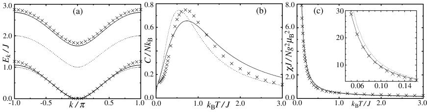
FIG. 1.: Dispersion relations of the ferromagnetic and antiferromagnetic elementary excitations (a) and temperature dependences of the specific heat (b) and the magnetic susceptibility (c) for the $(S,s)=(1,\frac{1}{2})$ ferrimagnetic Heisenberg chain. The linear (dotted lines) and interacting (solid lines) spin-wave calculations are compared with quantum Monte Carlo estimates.

where $E_{i}$ and $\omega_{i}^{\pm}$ are the $O(S^{i})$ quantum corrections to the dispersion relations. There exist two branches of spin waves in ferrimagnets, one of which reduces the ground-state magnetization and is thus of ferromagnetic aspect, while the other of which enhances the ground-state magnetization and is thus of antiferromagnetic aspect. The ferromagnetic and antiferromagnetic spin waves convincingly exhibit a quadratic dispersion and a gapped spectrum, respectively, as is shown in Fig. 1(a).

While the formulation is detailed in Ref. [38], we here mention the core idea of our ferrimagnetic modified spin-wave theory$-$how to control the number of bosons. The zero-magnetization constraint, which works well in ferromagnets, is not relevant to antiferromagnetically coupled spins, keeping constant the difference between the numbers of the sublattice bosons instead of the sum of them. Then we may consider that the staggered magnetization should be kept constant and introduce an alternative constraint as

$$\sum_{\sigma=\pm}\sum_{k}\frac{(S+s)\bar{n}_{k}^{\sigma}}{\sqrt{(S-s)^{2}+4Ss\sin^{2}(ak)}}=(S+s)N\,,$$ (16)

where $\bar{n}_{k}^{-}=\langle\alpha_{k}^{\dagger}\alpha_{k}\rangle$ and $\bar{n}_{k}^{+}=\langle\beta_{k}^{\dagger}\beta_{k}\rangle$. Equation (16) claims that the thermal fluctuation should cancel the staggered magnetization. The thus-calculated thermal quantities are shown in Fig. 1. The ferromagnetic features of ferrimagnets at low temperatures, the $T^{1/2}$-vanishing specific heat and the $T^{-2}$-diverging susceptibility, are reproduced well. The inset in Fig. 1(c) shows that the interacting modified spin-wave description is highly precise at sufficiently low temperatures. As for the specific heat, the inclusion of the spin-wave interactions corrects the position of the Schottky peak, which is consistent with the observations of Fig. 1(a).

There are many model compounds for the Hamiltonian (9). Kahn et al. [39] systematically synthesized spin-$(S,\frac{1}{2})$ quasi-one-dimensional ferrimagnets composed of two kinds of transition metals. More complicated alignments of mixed spins [40, 41] were also synthesized and investigated in terms of modified spin waves.

III Double-Peaked Specific Heat

The ferromagnetic and antiferromagnetic excitations coexistent in one-dimensional ferrimagnets lead to the mixed features of the specific heat: the $T^{1/2}$ initial behavior but the Schottky-type peak at mid temperatures. More interesting energy structure may be expected in ferrimagnets. Weak magnetic field applied to ferrimagnets indeed causes a double-peaked specific heat [42]. When the antiferromagnetic gap lies far apart from the lower-lying ferromagnetic band, there is a possibility of such observations in isotropic systems without any field and anisotropy. In the case of alternating-spin chains illustrated in Fig. 2(a), the linear spin-wave theory suggests the criterion as $S\gg 2s$. A series of bimetallic chain compounds [39] is interesting in this context, but even a combination of Mn ($S=\frac{5}{2}$) and Cu ($s=\frac{1}{2}$) turns out not enough for a double-peaked structure of the specific heat [43].

Metals of different kinds are not necessary to ferrimagnets. Caneschi et al. [44] synthesized hybrid ferrimagnets comprising metals and organic radicals. There are further solutions to ferrimagnets. Figures 2(b) and 2(c) illustrate ferrimagnets of topological origin [45, 46], which possibly exhibit a double-peaked specific heat [47]. Figure 3 shows the modified spin-wave calculations for the spin-$\frac{1}{2}$ trimeric chains depicted in Fig. 2(b) with particular emphasis on clarifying how an extra peak grows. The present scheme has the advantage of visualizing each excitation mode making a distinct contribution to the thermal behavior. As the ratio $J_{2}/J_{1}$ moves away from unity, the system begins to divide into small clusters and every excitation mode becomes less dispersive. With a sufficiently small but finite ratio, an extra peak appears at low temperatures. The model compound Sr₃Cu₃(PO₄)₄ indeed exhibits a double-peaked specific heat satisfying the condition $J_{2}/J_{1}\simeq 0.1$ [45]. A double-peaked specific heat is possible for the tetrameric chains depicted in Fig. 2(c) as well [47]. Extensive measurements on the model compound Cu(3-Clpy)₂(N₃)₂ (3-Clpy $=$ $3$-chloropyridine) [46, 48] and its analogs are encouraged.

Considering the difficulty of calculating thermodynamic properties at very low temperatures by numerical tools such as quantum Monte Carlo and density-matrix renormalization-group methods, the modified spin-wave scheme can play an effective role in investigating low-dimensional magnets as well. We can clearly understand what type of fluctuations is relevant to the phenomena of our interest in terms of spin waves. Indeed any spin-wave description is trivially less quantitative in systems with strong bond alternation and/or frustration [49], but there may be an idea that quantum phase transitions can be detected through the breakdown of spin-wave ground states [29, 30].

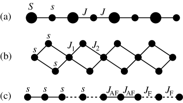
FIG. 2.: Schematic representations of bimetallic chain compounds (a), trimeric intertwining double-chain compounds (b), and tetrameric bond-alternating chain compounds (c), where smaller and larger bullet symbols denote spins $s=\frac{1}{2}$ and $S>\frac{1}{2}$, while solid and dashed segments mean antiferromagnetic and ferromagnetic exchange couplings between them, respectively.

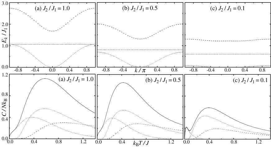
FIG. 3.: The interacting spin-wave calculations of the dispersion relations (the upper three) and the specific heat (the lower three) of the trimeric chains illustrated in Fig. 2(b), where individual contributions of the ferromagnetic and antiferromagnetic spin waves are distinguishably shown by dotted and dashed lines, respectively, the sum of which is equal to the total drawn by solid lines.

IV Nuclear Spin-Lattice Relaxation in Ferrimagnets

Next we consider observing ferrimagnets through nuclear spins. In the case of a bimetallic chain compound NiCu(pba)(H₂O)₃$\cdot$$2$H₂O (pba $=$ $1,3$-propylenebis(oxamato)) synthesized by Kahn et al. [39], proton nuclei lying apart from electronic spins effectively work as probes to illuminate the correlation between spins of different kinds peculiar to ferrimagnets. Considering the electronic-nuclear energy-conservation requirement, the Raman process should play a leading role in the nuclear spin-lattice relaxation. The Raman relaxation rate is generally given by

$$\frac{1}{T_{1}}=\frac{4\pi\hbar(g\mu_{\rm B}\gamma_{\rm N})^{2}}{\sum_{i}{\rm e}^{-E_{i}/k_{\rm B}T}}\sum_{i,f}{\rm e}^{-E_{i}/k_{\rm B}T}$$ (17)

$$\ \times\big{|}\langle f|\sum_{n}(A_{n}S_{n}^{z}+B_{n}s_{n}^{z})|i\rangle\big{|}^{2}\,\delta(E_{f}-E_{i}-\hbar\omega_{\rm N})\,,$$ (18)

where $A_{n}$ and $B_{n}$ are the dipolar hyperfine coupling constants between the nuclear and electronic spins in the $n$th unit cell, $\omega_{\rm N}\equiv\gamma_{\rm N}H$ is the Larmor frequency of the nuclei with $\gamma_{\rm N}$ being the gyromagnetic ratio, and the summation $\sum_{i}$ is taken over all the electronic eigenstates $|i\rangle$ with energy $E_{i}$. Taking account of the significant difference between the electronic and nuclear energy scales ($\hbar\omega_{\rm N}\lesssim 10^{-5}J$), Eq. (18) is expressed in terms of modified spin waves as [50]

$$\frac{1}{T_{1}}\simeq\frac{4\hbar(g\mu_{\rm B}\gamma_{\rm N})^{2}}{\pi J}\int_{0}^{\pi}{\rm d}k\frac{S-s}{\sqrt{(Ssk)^{2}+2(S-s)Ss\hbar\omega_{\rm N}/J}}$$ (19)

$$\qquad\times\bigl{[}(A{\rm cosh}^{2}\theta_{k}-B{\rm sinh}^{2}\theta_{k})^{2}\bar{n}_{k}^{-}(\bar{n}_{k}^{-}+1)$$ (20)

$$\qquad+(A{\rm sinh}^{2}\theta_{k}-B{\rm cosh}^{2}\theta_{k})^{2}\bar{n}_{k}^{+}(\bar{n}_{k}^{+}+1)\bigr{]}\,,$$ (21)

where $A$ and $B$ are the Fourier transforms of the coupling constants on the assumption that their momentum dependence can be neglected [51].

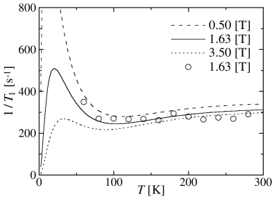
FIG. 4.: Temperature dependences of the proton spin-lattice relaxation rate with varying field for the $(S,s)=(1,\frac{1}{2})$ ferrimagnetic model compound NiCu(pba)(H₂O)₃$\cdot$$2$H₂O. The interacting modified spin-wave calculations, where $A=1.8\times 10^{-2}$ $\mbox{\AA}^{-3}$ and $B=5.9\times 10^{-2}$ $\mbox{\AA}^{-3}$, are compared with measurements ($\circ$) [51].

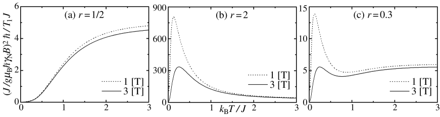
FIG. 5.: Temperature dependences of the nuclear spin-lattice relaxation rate with varying field for the $(S,s)=(1,\frac{1}{2})$ ferrimagnetic Heisenberg chain calculated in terms of the interacting modified spin waves.

In Fig. 4 the thus-calculated relaxation rate [52] is compared with experimental findings [51]. We have determined the coupling constants so as to well reproduce the observations under the condition that the probe protons are located closer to Cu than Ni [39]. Through the relations $A\sim d_{S}^{-3}$ and $B\sim d_{s}^{-3}$, where $d_{S}$ ($d_{s}$) is the average distance between the protons and the Ni (Cu) site in each unit, we obtain rough estimates $d_{S}\simeq 3.8\,[\mbox{\AA}]$ and $d_{s}\simeq 2.6\,[\mbox{\AA}]$, which are consistent with structural analyses [39]. However, the calculated field dependence is much weaker than the observations [51]. The field dependence can be better interpreted by the direct process [53] than by the Raman process. Since there are few nuclear-magnetic-resonance measurements on one-dimensional ferrimagnets, we hope that further explorations will be made from both chemical and physical points of view.

Apart from particular materials, we discuss the ferrimagnetic relaxation more generally. When we compare Eq. (21) with the expression of the susceptibility-temperature product [38],

$$\chi T=\frac{(g\mu_{\rm B})^{2}}{3k_{\rm B}}\sum_{k}\sum_{\sigma=\pm}\bar{n}^{\sigma}_{k}(\bar{n}^{\sigma}_{k}+1)\,,$$ (22)

we find that the ferromagnetic and antiferromagnetic excitations interestingly make varying contribution to $1/T_{1}$ according to the location of probe nuclei. Decreasing and increasing $\chi T$ with increasing temperature are characteristic of ferro- and antiferromagnets, respectively, and ferrimagnetic $\chi T$ exhibit a minimum. As long as we observe ferrimagnetism through the susceptibility, it looks like a uniform mixture of ferro- and antiferromagnetism. On the other hand, nuclear spins can selectively extract ferro- and antiferromagnetic features from ferrimagnets according to their location. We show in Fig. 5 the relaxation rate as a function of $A/B\equiv r$. The nuclei lie closer to larger (smaller) spins $S$ ($s$) for $r>1$ ($r<1$). Equation (21) claims that ferromagnetic (antiferromagnetic) spin waves can not mediate the nuclear spin relaxation at all for $r=\mbox{tanh}^{2}\theta_{k}$ ($r=\mbox{coth}^{2}\theta_{k}$). Considering the predominant contribution of $k\simeq 0$ to the integration (21) at low temperatures and weak fields [52], the nuclear spins correlate only to antiferromagnetic (ferromagnetic) spin waves at $r\simeq s/S$ ($r\simeq S/s$). Figures 5(a), 5(b), and 5(c) indeed present antiferromagnetic, ferromagnetic, and mixed-magnetic features, respectively, where vanishing rates at low temperatures in Figs. 5 (b) and 5(c) are due to the Zeeman interaction and should therefore be distinguished from the intrinsic properties. Since antiferromagnetic spin waves are hardly excited at low temperatures, nuclear spins located so as to satisfy the condition $r\sim(d_{s}/d_{S})^{3}\simeq s/S$ exhibit extremely slow dynamics.

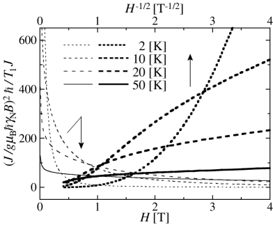
FIG. 6.: Field dependences of the nuclear spin-lattice relaxation rate with varying temperature for the $(S,s)=(1,\frac{1}{2})$ ferrimagnetic Heisenberg chain calculated in terms of the interacting modified spin waves, where $J/k_{\rm B}=121$ K and $r=0$.

Another interest in Eq. (21) is its field dependence. While it is usual for the relaxation rate to depend on an applied field through the electronic Zeeman energy, here is further field dependence in the prefactor. This novel field dependence originates in the quadratic dispersion relation of ferrimagnets and may arise from any nonlinear dispersion at the band bottom in more general. In Fig. 6 we show the relaxation rate as a function of an applied field, setting the parameters for NiCu(pba)(H₂O)₃$\cdot$$2$H₂O [39]. At low temperatures and moderate fields, $1/T_{1}$ behaves like $\propto 1/\sqrt{H}$, where $\bar{n}_{k}^{-}$ exhibits a sharp peak at $k=0$ and thus the integration (21) can be approximately replaced by the $k=0$ contribution. With increasing temperature, the predominant $k=0$ contribution smears and the $k$ integration ends up with a logarithmic field dependence. With increasing field, these unique observations are all masked behind the overwhelming Zeeman effect. The $1/\sqrt{H}$ dependence of our interest should be distinguished from the diffusion-dominated dynamics [54, 55, 56], which appears at high temperatures originating from transverse spin fluctuations. We hope that ferrimagnetic dynamics in a field will be more and more studied from the experimental point of view.

V Nanoscale Molecular Magnets

Mesoscopic magnetism [57] is one of the hot topics in materials science, where we can observe a dimensional crossover on the way from molecular to bulk magnets [58]. Metal-ion magnetic clusters are thus interesting and among others is [Mn₁₂O₁₂(CH₃COO)₁₆(H₂O)₄] [59] (hereafter abbreviated as Mn₁₂), for which quantum tunneling of the magnetization [60, 61] was observed for the first time. Figure 7 illustrates the Mn₁₂ cluster, where four inner Mn⁴⁺ spins and eight outer Mn³⁺ spins are directed antiparallel to each other and exhibit a novel ground state of total spin $S=10$ [62]. Assuming the stability of the collective spin of $S=10$, the Mn₁₂ cluster is often treated as a single spin-$10$ object [63]. However, recent electron-paramagnetic-resonance measurements [64] suggest a possible breakdown of the spin-$10$ description even at low temperatures. We have to consider the intracluster magnetic structure for further understanding of nanoscale magnets. Since NMR measurements on the Mn₁₂ cluster have recently made remarkable progress [65, 66, 67, 68, 69], we consider a microscopic interpretation [70] of them.

The total spin states in the Mn₁₂ cluster is too large even for modern computers to directly handle. Indeed several authors [71, 72] have recently succeeded in obtaining the low-lying eigenstates of the microscopic Hamiltonian, yet very little is known about the intracluster magnetic structure. There are four types of exchange interactions between the Mn ions forming the Mn₁₂ cluster, as is illustrated in Fig. 7, but their values are still the subject of controversy. Taking account of the current argument, we consider three possible sets of parameters. The Hamiltonian is defined as [73]

$${\cal H}=-\sum_{n=1}^{4}\Bigl{[}2J_{1}\mbox{\boldmath$s$}_{n}\cdot\mbox{\boldmath$S$}_{n}+2J_{2}(\mbox{\boldmath$s$}_{n}\cdot\mbox{\boldmath$\widetilde{S}$}_{n}+\mbox{\boldmath$\widetilde{S}$}_{n}\cdot\mbox{\boldmath$s$}_{n+1})$$ (23)

$$\quad+2J_{3}(\mbox{\boldmath$s$}_{n}\cdot\mbox{\boldmath$s$}_{n+1}+\frac{1}{2}\mbox{\boldmath$s$}_{n}\cdot\mbox{\boldmath$s$}_{n+2})$$ (24)

$$\quad+2J_{4}(\mbox{\boldmath$S$}_{n}\cdot\mbox{\boldmath$\widetilde{S}$}_{n}+\mbox{\boldmath$\widetilde{S}$}_{n}\cdot\mbox{\boldmath$S$}_{n+1})$$ (25)

$$\quad+D_{2}(S_{n}^{z})^{2}+D_{3}(\widetilde{S}_{n}^{z})^{2}+g\mu_{\rm B}H(s_{n}^{z}+S_{n}^{z}+\widetilde{S}_{n}^{z})\Bigr{]}\,,$$ (26)

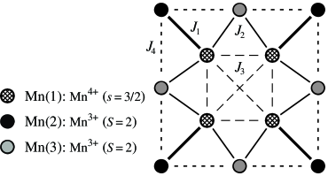
FIG. 7.: Schematic plot of the Mn₁₂ cluster.

where $\mbox{\boldmath$s$}_{n}$, $\mbox{\boldmath$S$}_{n}$, and $\widetilde{\mbox{\boldmath$S$}}_{n}$ are the spin operators for the Mn(1) (spin $\frac{3}{2}\equiv s$), Mn(2) (spin $2\equiv S$), and Mn(3) (spin $2\equiv S$) sites in the $n$th unit, respectively. The parameter sets (a), (b), and (c) listed in Table I are based on the calculations in Refs. [74], [73], and [72], respectively. The early arguments (a) and (b) agree on $J_{1}$ predominating over the rest, which is supported by recent calculations [70, 71], whereas the latest claim (c) is completely against such a consensus, throwing doubt on previous investigations such as the eight-spin modeling of the Mn₁₂ cluster [75]. As for the anisotropy parameters, there is much less information. When the molecule is treated as a rigid spin-$10$ object, the macroscopic uniaxial crystalline anisotropy parameter $D$ is determined so as to fit the zero-field separation between the lowest two levels, ${\mit\Delta}\simeq 14\,\mbox{K}$ [62, 73]. Hence it is natural to choose the local single-ion anisotropy parameters $D_{2}$ and $D_{3}$, describing the Jahn-Teller-distorted Mn³⁺ ions [76], within the same scheme.

We introduce the bosonic operators within the linear spin-wave scheme as $s_{n}^{z}=-s+a_{n,1}^{\dagger}a_{n,1}$, $s_{l}^{+}=\sqrt{2s}a_{n,1}^{\dagger}$; $S_{n}^{z}=S-a_{n,2}^{\dagger}a_{n,2}$, $S_{n}^{+}=\sqrt{2S}a_{n,2}$; $\widetilde{S}_{n}^{z}=S-a_{n,3}^{\dagger}a_{n,3}$, $\widetilde{S}_{n}^{+}=\sqrt{2S}a_{n,3}$, which can be justified in the low-temperature range where ⁵⁵Mn NMR measurements [67, 68, 69] are performed. While the same type constraint as Eq. (16) is given by

$$\sum_{k}\sum_{n=1,2,3}\bar{n}_{k,n}\sum_{m=1,2,3}|\psi_{mn}(k)|^{2}=8S+4s\,,$$ (27)

providing we define the Bogoliubov transformation as

$$\left.\begin{array}[]{rrrr}a_{k,1}=&-\psi_{11}(k)\,b_{k,1}^{\dagger}&-\psi_{12}(k)\,b_{k,2}^{\dagger}&+\psi_{13}(k)\,b_{k,3}\,,\\ a_{k,2}=&\psi_{21}^{*}(k)\,b_{k,1}&+\psi_{22}^{*}(k)\,b_{k,2}&-\psi_{23}^{*}(k)\,b_{k,3}^{\dagger}\,,\\ a_{k,3}=&\psi_{31}^{*}(k)\,b_{k,1}&+\psi_{32}^{*}(k)\,b_{k,2}&-\psi_{33}^{*}(k)\,b_{k,3}^{\dagger}\,,\\ \end{array}\right.$$ (28)

this is not applicable to the Mn₁₂ cluster as it is. In isotropic ferrimagnets, there exists a zero-energy excitation and therefore a certain number of bosons naturally survive at low temperatures. Once a gap $\mit\Delta$ opens, which is the case of the anisotropic Mn₁₂ clusters, the boson number should exponentially decreases as $\propto{\rm e}^{-{\mit\Delta}/k_{\rm B}T}$ at low temperatures, but the constraint (27) still keeps it finite even at $T\rightarrow 0$. Hence we replace Eq. (27) by

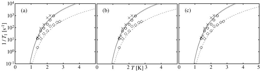
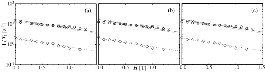
FIG. 8.: Semilog plots of the ⁵⁵Mn nuclear spin-lattice relaxation rates as functions of temperature under no field for the parameter sets listed in Table I. The linear modified spin-wave calculations, dashed [Mn(1)], dotted [Mn(2)], and solid [Mn(3)] lines, are compared with measurements [67], $\diamond$ [Mn(1)], $\circ$ [Mn(2)], and $\times$ [Mn(3)].

FIG. 9.: Semilog plots of the ⁵⁵Mn nuclear spin-lattice relaxation rates as functions of an applied field at $T=1.4$ K for the parameter sets listed in Table I. The linear modified spin-wave calculations, dashed [Mn(1)], dotted [Mn(2)], and solid [Mn(3)] lines, are compared with measurements [67], $\diamond$ [Mn(1)], $\circ$ [Mn(2)], and $\times$ [Mn(3)].

$$\sum_{k}\sum_{n=1,2,3}\bar{n}_{k,n}\sum_{m=1,2,3}|\psi_{mn}(k)|^{2}=(8S+4s)\,{\rm e}^{-{\mit\Delta}/k_{\rm B}T}\,.$$ (29)

This is quite natural modification of the theory, because the new constraint (29) remains the same as the authorized one (27) except for the sufficiently low-temperature region $k_{\rm B}T\lesssim{\mit\Delta}$. It is also convincing that Eq. (29) smoothly turns into Eq. (27) as ${\mit\Delta}\rightarrow 0$.

The thus-calculated Raman relaxation rates for the ⁵⁵Mn nuclei as functions of temperature and an applied field are compared with measurements [67] in Figs. 9 and 9, where the coupling constants $A_{i}$ are the only adjustable parameters in reproducing both temperature and field dependences and have been chosen as Table II. The parameter set (b) best agrees to the experimental findings. At the same time, we are surprised to learn that the latest argument (c) is also reasonable. Since the present calculations are not so quantitative as to distinguish the two scenarios (b) and (c), the intracluster magnetic structure should be reexamined in all its aspects. The assumption of the leading Raman process is less trivial for the Mn⁴⁺ ions. A recent experiment [68] suggests that the hyperfine field of the Mn³⁺ ions is in fact anisotropic and makes a predominant dipolar contribution, whereas that of the Mn⁴⁺ ions is isotropic and results in the Fermi contact. In this context, it is interesting to compare carefully the theoretical ($A_{i}^{\rm th}$) and experimental ($A_{i}^{\rm ex}$) findings for the coupling constants. Assuming the set (b), $A_{1}^{\rm th}\simeq 2.5A_{1}^{\rm ex}$, $A_{2}^{\rm th}\simeq 1.7A_{2}^{\rm ex}$, and $A_{3}^{\rm th}\simeq 1.2A_{3}^{\rm ex}$. Somewhat larger deviation of the theory from the experiment for $A_{1}$ implies that the nuclear spin-lattice relaxation on the Mn(1) site may not be Raman active primarily but be strongly influenced by the surrounding Mn³⁺ ions. The present theory is distinct from the phenomenological interpretation [65] assuming phonons to mediate the relaxation. We hope microscopic investigations of this kind will contribute toward the total understanding of mesoscopic magnetism.

VI Spin-Gapped Antiferromagnets

We have fully discussed the systems with macroscopically degenerate magnetic ground states, where the difficulty of diverging number of bosons does not occur unless temperature is sufficiently high. From this point of view, one-dimensional antiferromagnets are harder for spin waves to treat, where the problem lies already in the ground state. However, here are not a few interesting systems such as Haldane-gap antiferromagnets [77] and antiferromagnetic spin ladders [78]. The antiferromagnetic modified spin-wave theory is not so successful as that for ferro- and ferrimagnets, but it can still play a helpful role in our explorations. We close our discussion by demonstrating bosonic treatments of integer-spin Heisenberg chains [79].

We are expected to avoid the quantum divergence of sublattice magnetizations maintaining the core idea of constant bosons in number. We introduce the sublattice bosons as Eq. (11), where $S=s$, and diagonalize an effective Hamiltonian

$$\widetilde{\cal H}={\cal H}+2J\lambda\sum_{n}(a_{n}^{\dagger}a_{n}+b_{n}^{\dagger}b_{n})\,,$$ (30)

instead of ${\cal H}$, where the Lagrange multiplier $\lambda$ is determined by the condition

$$\sum_{n}a_{n}^{\dagger}a_{n}=\sum_{n}b_{n}^{\dagger}b_{n}=SN\,.$$ (31)

Within the conventional spin-wave theory, spins on one sublattice point predominantly up, while those on the other predominantly down. The constraint (31) restores the sublattice symmetry.

It is interesting to compare the modified spin-wave scheme with another bosonic approach. The Schwinger-boson representation of the spin algebra [80, 81] is also a common language to interpret quantum magnetism and its application to one-dimensional systems [82, 83] is moving ahead recently. Let us describe each spin variable in terms of two kinds of bosons as

$$S_{l}^{+}=a_{l\uparrow}^{\dagger}a_{l\downarrow}\,,\ S_{l}^{-}=a_{l\downarrow}^{\dagger}a_{l\uparrow}\,,\ S_{l}^{z}=\frac{1}{2}\bigl{(}a_{l\uparrow}^{\dagger}a_{l\uparrow}-a_{l\downarrow}^{\dagger}a_{l\downarrow}\bigr{)}\,,$$ (32)

where we impose the constraint

$$a_{l\uparrow}^{\dagger}a_{l\uparrow}+a_{l\downarrow}^{\dagger}a_{l\downarrow}=2S\,,$$ (33)

on the bosons. At the mean-field level, we diagonalize the Hamiltonian with the constraints imposed on the average and obtain the dispersion relation as

$$\omega_{k}=2\sqrt{\lambda^{2}-\Omega^{2}\cos^{2}(ak)}\,,$$ (34)

where $\lambda$ and $\Omega$ are determined through

$$\left.\begin{array}[]{lll}{\displaystyle\sum_{k}\frac{2\lambda(2\bar{n}_{k}+1)}{\sqrt{\lambda^{2}-\Omega^{2}\cos^{2}(ak)}}}&=&(2S+1)L\,,\\ {\displaystyle\sum_{k}\frac{(2\bar{n}_{k}+1)\cos^{2}(ak)}{\sqrt{\lambda^{2}-\Omega^{2}\cos^{2}(ak)}}}&=&L\,,\end{array}\right.$$ (35)

with $\bar{n}_{k}=[{\rm e}^{\omega_{k}/k_{\rm B}T}-1]^{-1}$. The magnetic susceptibility is expressed as

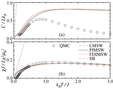
FIG. 10.: Temperature dependences of the specific heat (a) and the magnetic susceptibility (b) for the $S=1$ antiferromagnetic Heisenberg chain calculated by the linear modified spin waves (LMSW), the perturbational (PIMSW) and full-diagonalization (FDIMSW) interacting modified spin waves, the Schwinger bosons (SB), and a quantum Monte Carlo method (QMC).

$$\chi=\frac{(g\mu_{\rm B})^{2}}{k_{\rm B}T}\sum_{k}\sum_{\sigma=\pm}\bar{n}_{k}(\bar{n}_{k}+1)\,,$$ (36)

while the internal energy as

$$E=JL\bigl{[}S^{2}+2\Omega^{2}-2\lambda(2S+1)\bigr{]}+2\sum_{k}(2\bar{n}_{k}+1)\omega_{k}\,,$$ (37)

where we have corrected the mean-field artifact [80] of double counting the degrees of freedom for the Schwinger bosons.

In Table III all the present findings for the ground-state energy and the lowest excitation gap are compared with quantum Monte Carlo calculations [84]. As for the modified spin-wave calculations, we can treat the $O(S^{0})$ correlations in two different ways. One idea is the perturbational treatment of ${\cal H}_{0}$ to ${\cal H}_{1}$, which is referred to as the perturbational interacting modified spin-wave scheme, while the other is the full diagonalization of ${\cal H}_{1}+{\cal H}_{0}$, which is referred to as the full-diagonalization interacting modified spin-wave scheme. On the whole, the bosonic languages well represent the ground-state energy but fail to describe the Haldane gap quantitatively. However, they are still useful in understanding the nature of magnetic excitations. Although the modified spin waves underestimate the absolute value of the gap, they reproduce the observed temperature dependence of the Haldane gap [85] better than the nonlinear $\sigma$ model [79, 86]. Thus the spin-wave picture still looks valid for spin-gapped antiferromagnets. The Haldane-gap phase may be symbolically interpreted as a valence bond solid [87], but such a picture is not strictly valid for the pure Heisenberg Hamiltonian. In the case of spin $1$, for example, even a likely ground state of bound crackions [88, 89] moving in the valence-bond-solid background gives a variational energy [90] inferior to the interacting modified spin-wave estimates. It is also interesting that the full-diagonalization interacting modified spin waves and the mean-field Schwinger bosons give the same estimate of the Haldane gap. The Schwinger-boson dispersion relation (34) indeed coincides exactly with that of the full-diagonalization interacting modified spin waves at $T=0$. This is not so surprising because the Holstein-Primakoff bosons are obtained by replacing both $a_{l\uparrow}$ and $a_{l\uparrow}^{\dagger}$ by $(2S-a_{l\downarrow}^{\dagger}a_{l\downarrow})^{1/2}$ in the transformation (32).

On the other hand, the modified spin waves are definitely distinguished from the Schwinger bosons in thermal calculation. Their findings for the specific heat and the magnetic susceptibility are compared in Fig. 10. While the Schwinger-boson mean-field theory rapidly breaks down with increasing temperature, the modified spin waves still give useful information at finite temperatures. The modified spin-wave calculations well reproduce the overall behavior of the susceptibility converging into $\chi/Lg^{2}\mu_{\rm B}^{2}=S(S+1)/3k_{\rm B}T$ at high temperatures. We admit, however, that one of the fatal weak points in the modified spin-wave description of spin-gapped antiferromagnets is nonvanishing specific heat at high temperatures. It is not the case with ferro- and ferrimagnets provided we introduce the Lagrange multiplier in constructing thermodynamics. The endlessly increasing energy with increasing temperature is because of the temperature-dependent energy spectrum, where the Lagrange multiplier, playing the chemical potential, turns out a monotonically increasing function of temperature. Such a difficulty is common to all the bosonic approaches to spin-gapped antiferromagnets, where a fermionic language may be more effective [91, 92, 93].

VII Concluding Remarks

In the late 1980’s, the low-dimensional spin-wave theory made an epochal progress, where a problem pending in one-dimensional ferromagnets was solved and two-dimensional antiferromagnets were discussed in the context of high-temperature superconductivity. More than a decade has passed and the spin-wave theory has grown more useful and extensive covering one and possibly zero dimensions. There are further interesting investigations in terms of spin waves for ladder [93, 94, 95], frustrated [96], and random-bond [97] systems. The present findings can be reconstructed through the Dyson-Maleev transformation [3, 98] instead of the Holstein-Primakoff scheme. The modified spin-wave theory breaks the rotational symmetry anyway, while the Schwinger-boson representation [80, 81, 82] is rotationally invariant.

Considering the rich harvest [26, 38, 70] in the ferro- and ferrimagnetic modified spin-wave theory, the antiferromagnetic modified spin-wave scheme [27, 28, 79] is less successful in one dimension in particular, where the ground-state properties and the magnetic susceptibility are well calculated, while the energy gap and the specific heat are poorly reproduced. Recently the Jordan-Wigner spinless fermions defined along a snake-like path [91, 92, 93] gave a fine description of ladder antiferromagnets, a piece of which is listed in Table IV. We learn that the spin-gap is better reproduced by the spinless fermions. The bosonic and fermionic languages are complementary in our explorations of low-dimensional magnets. All these arguments stimulate further interest [100] in the spin-wave theory. The spin-wave scheme will be refined more and more in the 21st century.

TABLE I.: Possible exchange interactions for the Mn₁₂ cluster in the unit of $\mbox{cm}^{-1}$.

	$J_{1}$	$J_{2}$	$J_{3}$	$J_{4}$
(a)	$-150$	$-60$	$60$	$30$
(b)	$-150$	$-60$	$-30$	$30$
(c)	$-41$	$-41$	$3$	$-8$

TABLE II.: Estimates of the hyperfine interaction $g\mu_{\rm B}\gamma_{\rm N}A_{i}$ in the unit of $\mbox{rad}\cdot\mbox{Hz}$ between the nuclear and electronic spins on the Mn($i$) site. The linear modified spin-wave calculations are compared with experimental findings [67].

	Mn(1)	Mn(2)	Mn(3)
Theory (a)	$8.9\times 10^{8}$	$1.8\times 10^{9}$	$1.9\times 10^{9}$
Theory (b)	$2.5\times 10^{8}$	$5.1\times 10^{8}$	$5.4\times 10^{8}$
Theory (c)	$3.3\times 10^{8}$	$5.1\times 10^{8}$	$6.6\times 10^{8}$
Experiment	$1.0\times 10^{8}$	$3.0\times 10^{8}$	$4.5\times 10^{8}$

TABLE III.: The ground-state energy per spin $E_{\rm g}/L$ and the lowest excitation gap ${\mit\Delta}$ for the $S=1$ antiferromagnetic Heisenberg chain calculated by the linear modified spin waves (LMSW), the perturbational (PIMSW) and full-diagonalization (FDIMSW) interacting modified spin waves, the Schwinger bosons at the mean-field level (SB), and a quantum Monte Carlo method (QMC) [84].

	$E_{\rm g}/L$	${\mit\Delta}$
LMSW	$-1.361879$	$0.07200$
PIMSW	$-1.394853$	$0.07853$
FDIMSW	$-1.394617$	$0.08507$
SB	$-1.396148$	$0.08507$
QMC	$-1.401481(4)$	$0.41048(6)$

TABLE IV.: The ground-state energy per rung $E_{\rm g}/N$ and the lowest excitation gap ${\mit\Delta}$ for the $S=\frac{1}{2}$ antiferromagnetic Heisenberg two-leg ladder with intra- and interchain couplings of equal strength calculated by the spinless fermions within the Hartree (HSF) and Hartree-Fock (HFSF) approximations, the linear modified spin waves (LMSW), the perturbational interacting modified spin waves (PIMSW), and a density-matrix renormalization-group method (DMRG) [99].

	$E_{\rm g}/L$	${\mit\Delta}$
HSF	$-0.838805$	$0.500000$
HFSF	$-0.907183$	$0.450419$
LMSW	$-1.101403$	$0.100911$
IMSW	$-1.143750$	$0.112832$
DMRG	$-1.156086$	$0.504$