The effects of macroscopic inhomogeneities on the magneto transport properties of the electron gas in two dimensions

Abstract

In experiments on electron transport the macroscopic inhomogeneities in the sample play a fundamental role. In this paper and a subsequent one we introduce and develop a general formalism that captures the principal features of sample inhomogeneities (density gradients, contact misalignments) in the magneto resistance data taken from low mobility heterostructures. We present detailed assessments and experimental investigations of the different regimes of physical interest, notably the regime of semiclassical transport at weak magnetic fields, the plateau-plateau transitions as well as the plateau-insulator transition that generally occurs at much stronger values of the external field only.

It is shown that the semiclassical regime at weak fields plays an integral role in the general understanding of the experiments on the quantum Hall regime. The results of this paper clearly indicate that the plateau-plateau transitions, unlike the the plateau-insulator transition, are fundamentally affected by the presence of sample inhomogeneities. We propose a universal scaling result for the magneto resistance parameters. This result facilitates, amongst many other things, a detailed understanding of the difficulties associated with the experimental methodology of H.P. Wei et.al in extracting the quantum critical behavior of the electron gas from the transport measurements conducted on the plateau-plateau transitions.

I Introduction

Quantum phase transitions in the quantum Hall regime were first studied by H.P. Wei et al. wei:prl88 who demonstrated that the width $\Delta\nu(T)$ of the transitions between adjacent quantum Hall plateaus (PP transitions) becomes infinitely narrow as the temperature $T$ goes to zero. An algebraic behavior $\Delta\nu(T)\propto T^{\kappa}$ with $\kappa=0.42\pm 0.04$ was found, independent of the Landau levelwei:prl88 ; hwang:prb93 . This indicated that the PP transitions in the quantum Hall regime should be regarded as a quantum critical phenomenon with universal critical indicespruisken:prl88 .

An overwhelming majority of subsequent experiments, by many otherskoch ; shahar:ssc97 ; hilke:nat98 ; pi_expts , have primarily revealed the elusive character of the quantum phase transition. These experiments, unlike those by H.P. Wei et. al., were primarily conducted on arbitrarily chosen samples that did not provide any access to the quantum critical phenomenon, given the well known experimental limitations in reaching $T=0$. It is well understood, although still not generally recognized as such, that in order to be able to experimentally probe the true $T=0$ asymptotics of the quantum phase transition, the dominant scattering mechanism of the electron gas should be provided by short ranged potential fluctuations. Smoothly varying potential fluctuations (relative to the magnetic length) like those present in the $GaAs/AlGaAs$ heterostructure mainly give rise to an anomalously large crossover length scale for scaling such that quantum criticality cannot be retrieved in the experiment which is conducted at finite $T$. Crossover phenomena, especially those between percolation and localization, have in general remained difficult to grasp. Nevertheless, they do exist as an integral chapter in the renormalization theory of the quantum Hall effectpaperIII . These phenomena play a crucial and fundamental role in the understanding of not only laboratory experiments but also the numerical experiments on the plateau transitions in the quantum Hall regime.

Yet another complication is well known to play a major role, the presence of macroscopic sample inhomogeneities that are inherent to the experiments. Notice that spatial variations in the electron density mainly produce a spatially varying filling fraction $\nu$ of the Landau level. Any such macroscopic inhomogeneity in the electron density, no matter how small, will eventually complicate the critical behavior of the electron gas in the limit where $T$ and, hence, the width $\Delta\nu(T)$ of the plateau transitions goes to zero. The experimental situation is in many ways similar to that of an ordinary liquid-gas phase transition where, as is well known, inhomogeneity effects due to gravity prevents one from entering arbitrary deeply into the critical phase. Unlike the liquid gas phase transition, however, there hardly exists any detailed study or systematic knowledge on the inhomogeneity problem, especially in low mobility heterostructures. Transport measurements on the Hall bar geometry at low $T$ usually give rise to rather different results depending on the pairs of contacts that are being used, the polarity of the external field $B$ etc. Besides these geometrical aspects one generally observes also slight differences in the data taken from different experimental runs, before and after the sample has been heated up to room temperature ($T$) and then cooled down againschaijk:prl00 .

These annoying and puzzling complications have been the primary reason why the experiments on the Hall bar geometry have so far not provided any reliable information on the details of the scaling functions of the conductivity parameters in the transition regime between adjacent quantum Hall plateaus, notably the peak value and the shape of $\sigma_{xx}$. Moreover, the most important and fundamental aspect of the problem, the numerical value of the critical index $\kappa$, has remained an unsettled experimental problem. In spite of the fact that the original data of H.P. Wei et.al. have provided an impressive experimental demonstration of a quantum phase transition in the quantum Hall regime, over the largest possible range of experimental $T$, it has remained somewhat uncertain whether the extracted value of the exponent $\kappa=0.42\pm 0.04$ is in fact the true critical value, or whether it represents an effective exponent resulting from an admixture of quantum critical behavior and sample dependent effects due to macroscopic inhomogeneities.

Unexpected insights into the problem have been obtained more recentlypruisken:stretch , as a result of a series of detailed studies on quantum transport taken from the lowest Landau level (PI transition) of a low mobility $InP-InGaAs$ heterostructureschaijk:prl00 ; lang:phe02 , Quite contrary to the general statement which says that the basic phenomenon of quantum criticality is independent of the Landau level, there are, from an experimental point of view, fundamental and surprising differences. It turns out that the plateau-insulator or PI transition is generally much less affected by sample inhomogeneities than the plateau-plateau or PP transitions taken from the same sample. The difference primarily reveals itself in terms of previously unrecognized symmetries in the observed magneto resistance data under a change in the polarity of the external magnetic field $B$. Moreover, the PI transition, unlike the PP transitions, displays very specific and general features that permit one to disentangle the quantum critical aspects of the transport data (particle-hole symmetry, critical exponents, scaling functions) and those that are non-universal and sample dependent (gradients in the electron density, contact misalignments). As a result of all this, one can now say that the previously accepted experimental value of the exponent $\kappa=0.42$ is slightly incorrect. Instead, a new value has been obtained, $\kappa=0.57$. This new result indicates that the quantum critical phenomenon belongs to a new, non-Fermi-liquid universality class, in agreement with the more recent advancements of the theory of localization and interaction effects in the quantum Hall regimeEuroLett ; Finkel ; twoloop . At the same time, the new studies also indicate that the scaling functions of the transport parameters $\sigma_{xx}$ and $\sigma_{xy}$ are, in fact, universal and in accordance with the statement of self-duality under the Chern Simons mapping.

These surprising advances illuminate the problem of quantum criticality in the quantum Hall regime by revealing all the features sought in the PP transition that previously remained concealed. In this paper we elaborate on the new insights that one has gained from the studies of the PI transition and embark on the specific difficulties associated with the PP transitions. We set up a general, conceptual framework that enables one to not only recognize the effects of macroscopic inhomogeneities from the experimental data, but also perform the appropriate quantitative analyses. Following the findings of Ref.pruisken:stretch, there are two distinctly different physical mechanisms at work in the experiments. These mechanisms are

1. A linear gradient in the electron density across the Hall bar,

2. A misalignment of the contacts on the Hall bar.

Our main objective is to demonstrate, both experimentally and theoretically, that these physical mechanisms have a quite general significance for the electron gas. They describe the inhomogeneity effects in the transport data of not only the PI transition at strong values of $B$, but also the PP transitions at intermediately strong $B$ as well as the regime of semiclassical transport (or weak quantum interference regime) that generally occurs at weak values of $B$. We will show that the aforementioned mechanisms manifest themselves quite differently, with distinctly different physical consequences, in each regime of $B$ that one is interested in.

As a general remark we can say that the experiments on the PP transitions are most dramatically affected, even by relatively weak inhomogeneities in the electron density. Whereas in practice the complications are much less severe for both the PI transition and the semiclassical regime and the corrections are relatively simple, this is generally not the case for the PP transitions. The main reason is that the effects of density gradients appear with a strength proportional to $\partial\rho_{xy}/\partial B$, i.e. the derivative of the Hall resistance with respect to the external field. This quantity tends to diverge at the center of the PP transition as $T$ approaches absolute zero. These effects, however, are very weak in the semiclassical regime and even absent near the PI transition where the Hall resistance $\rho_{xy}$ remains quantized and equal to $h/e^{2}$ at low $T$. This, then, is the basic answer to the inhomogeneity problem stated at the outset. It summarizes, at the same time, the principal conclusions of this paper.

We already mentioned the fact that symmetries play an important role in this magneto resistance problem. For example, the recent analysis of the PI transition is based, to a large extend, on an idea borrowed from the renormalization theory of the quantum Hall effect which says that particle-hole symmetry is a fundamental aspect of quantum criticality in the quantum Hall regimepruisken:prl88 . This symmetry indicates, crudely speaking, that the lines $\sigma_{xy}=half-integer$ should emerge as axes of symmetry in the $\sigma_{xx}$ and $\sigma_{xy}$ conductivity plane. It has been known for a long time, however, that this symmetry is generally violated in the experiment at low $T$, due to the presence of macroscopic inhomogeneities in the samplewei:prb86 .

As far as the PP transitions are concerned, the standard way of dealing with this problem has been to ”average” over the transport data taken at opposite polarities of the external field $B$. This procedure cannot always be taken seriously, however, because the raw experimental data, especially at low $T$, usually deviates substantially from the ”averaged” value. In this paper we elaborate on yet another, previously unrecognized symmetry of the the PP transitionpono that enables one to distinguish amongst the effects of density gradients and, say, contact misalignments. This symmetry which we term reflection symmetry indicates that no new information is added to the Hall bar measurements if one changes the polarity of the $B$ field. More specifically, it says that under the change $B\rightarrow-B$ the different resistances, taken from the four terminals of the Hall bar, are in effect mapped onto one another.

We show that reflection symmetry is primarily the result of having linear gradients in the electron density across the Hall bar and, therefore, it generally stands for an approximate symmetry only. Nevertheless, it has experimental significance even when relatively large density gradients are present in the sample. Most importantly, however, it teaches us how to proceed in order to physically understand and describe the difficult inhomogeneity problems that are associated with the PP transitions.

This paper is organized as follows. In Section 2 we outline a theoretical analysis of density gradients in Hall bar samples on the results of magneto transport experiments. Initially we consider linear density gradients (Section 2.2) and obtain explicit correction terms for the longitudinal and transverse resistances. These reveal an important property - reflection symmetry - in the magneto resistances taken from different contact pairs, with reversal of the magnetic field polarity. These results are directly applicable to the transport measurements on the semiclassical regime (Section 3.2). Going beyond the linear approximation, Section 2.3 presents the result of an exactly solvable nonlinear problem involving exponential density gradients. This analysis provides estimates of higher order corrections due to nonlinear gradients in the semiclassical regime. Gradient effects and related symmetry properties in the high $B$ regime are also obtained. In Section 2.4 we explore the sensitivity of the quantum critical behavior at the PP and PI transitions to density gradients. This leads to specific limits on the maximum density gradients which must be satisfied for meaningful investigations of quantum criticality. Finally, in Section 2.5, we discuss the recently reported experimental results on universality of the scaling functions of the PI transitions. We show, in particular, how they become generally useful in dealing with the more difficult problems that are associated with the experiments on the PP transitions. For this purpose we recapitulate some of the principle advances in the theory of localization and interaction effects in the quantum Hall regime (Appendix) and propose explicit scaling results for the PP transitions (Eqs 84 and 85).

In Section 3 we apply the results of Section 2 to the experimental resistance data taken from a low mobility $InGaAs$ quantum well. The low B, semiclassical transport data display many features expected from samples having linear density gradients, most prominent being the reflection symmetries. We show how the true transport parameters can be extracted that are free from inhomogeneity effects. These in turn are shown to be useful, in Section 3.2, for the investigation of (i) the departure from the semicircle law in the $\sigma_{xx}$, $\sigma_{xy}$ conductivity plane, (ii) the effects of weak quantum interference and (iii) the effects of higher order, nonlinear behavior due to density gradients. Section 3.3 describes the experimental results on the quantum Hall regime, bringing out the symmetry properties, as well as the limitations posed by the large density gradients in getting information about the quantum critical behavior of the PP transitions. In addition, the effects of contact misalignments are presented. Finally, in Section 4, we present a summary of the results and the main conclusions of this paper.

II Density gradients

II.1 Introduction

Density gradients in Hall bars, as well as other macroscopic inhomogeneities such as contact misalignments etc., are long standing experimental problems that are hard to deal with in detail and difficult to control in general. The analysis that follows is based on the assumption which says that the spatial extend of macroscopic inhomogeneities is typically much, much larger than any of the microscopic or mesoscopic length scales in the problem of transport of two dimensional electrons. Under these circumstances one can apply the results of ordinary electrodynamics. This means that one can describe the transport process by assuming phenomenological transport equations with slowly varying, position dependent transport coefficients. The general problem is actually a very old oneinhomogeneity and, as is well known, the complications are very specific to the magneto resistance measurements and usually do not arise in ordinary problems of quantum transport, in zero magnetic field $B$.

It is important to emphasize that our physical objectives have nothing to do with, say, the mesoscopic type of ideas on sample inhomogeneitypercol that are inspired by Landau level systems with smoothly varying, long ranged potential fluctuations. For the low mobility samples that are of interest to us, semiclassical ideas based on the percolation picture only enter the problem in a fictitious regime of extremely low $T$ where, as we mentioned before, the experiment on quantum criticality has been completely destroyed, as a result of inhomogeneities in the sample. Quite obviously, the physical objectives of scaling, at finite $T$, simply demand that one starts the analysis from the opposite limit where the effects of macroscopic inhomogeneities are negligibly small. Indeed, one of the most important and difficult tasks that one is faced with is to make sure that the experiment is conducted in a regime in $T$ where the sample inhomogeneities hardly affect the basic phenomena of interest such that the appropriate corrections can be made.

Imagine a local density $\bf j$ of DC electrical current that in principle may flow anywhere in the bulk of the sample as long as certain local and macroscopic constraints are satisfied. The conservation of charge is expressed by the continuity equation ${\bf\nabla}\cdot{\bf j}=0$. This implies that the total electrical current $\bf J$ through the Hall bar is constant and independent of the coordinate $x$ along the Hall bar (Fig. 1). Next, the condition for having a stationary state can be expressed using Maxwell’s equation $\partial{\bf B}/\partial t={\bf\nabla}\times{\bf E}=0$. Alternatively, we may apply Stoke’s theorem, $\oint{\bf E.dl}$ = 0, which says that no source of voltage should exist inside the the Hall bar.

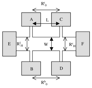
Figure 1: Schematic diagram of Hall bar, L = 1mm, W = 0.5 mm

The phenomenological transport equations can be written in the standard form

$$E_{x} = ~{}~{}\rho_{0}j_{x}-\rho_{H}j_{y}$$ (1)

$$E_{y} = ~{}~{}\rho_{H}j_{x}+\rho_{0}j_{y},$$ (2)

Here $\rho_{0}$ and $\rho_{H}$ denote the longitudinal and transversal or Hall resistivity respectively which may be taken as phenomenological parameters that vary slowly in $x$ and $y$. The aforementioned constraints imply that current density ${\bf j}=(j_{x},j_{y})$ satisfies the following equations

$${\bf\nabla}\cdot{\bf j} = 0$$ (3)

$$\rho_{0}{\bf\nabla}\times{\bf j} = (\partial_{y}\rho_{0}-\partial_{x}\rho_{H})j_{x}-(\partial_{x}\rho_{0}+\partial_{y}\rho_{H})j_{y}.$$ (4)

By writing ($j_{x}$ , $j_{y}$) = ($\partial_{y}\phi$ , $-\partial_{x}\phi$) we can also express Eqs (3) and (4) in terms of a differential equation for the scalar field $\phi$ alone,

$${\rho_{0}}{\Delta\phi}=-\left[(\partial_{x}\rho_{0}+\partial_{y}\rho_{H})\partial_{x}+(\partial_{y}\rho_{0}-\partial_{x}\rho_{H})\partial_{y}\right]\phi.$$ (5)

II.2 Linear approximation

II.2.1 Formalism

Except for the very special cases to be discussed below it is not only difficult to solve Eq. (5) in general but also very hard to extract relevant and physical information by pursuing a purely analytic approach to the problem. It is important to keep in mind, however, that we are primarily interested in the effects that are induced by weak macroscopic inhomogeneities. An adequate description of the problem is obtained by employing what we call the linear approximation. This amounts to having transport parameters $\rho_{0}$ and $\rho_{H}$ that vary linearly in the coordinates $x$ and $y$ according to

$$\rho_{0} = \rho_{0}^{0}(1+\alpha_{x}x+\alpha_{y}y)$$ (6)

$$\rho_{H} = \rho_{H}^{0}(1+\beta_{x}x+\beta_{y}y).$$ (7)

Here, the $\alpha^{\prime}s$ and $\beta^{\prime}s$ are given as phenomenological parameters that may vary with $T$ and the external field $B$ etc. We assume for simplicity a rectangular geometry of length $L$ (x-direction) and width $W$ (y-direction, see Fig. 1). The coordinates $x$ and $y$ are defined relative to the center of the Hall bar. It is easy to see that a spatially varying current density of the form

$$j_{x} = j_{x}^{0}(1+a_{y}y)$$

$$j_{y} = 0$$ (8)

satisfies all the aforementioned constraints and boundary conditions. Working to linear order in the coordinates $x$ and $y$ one can write the transport equations as follows

$$E_{x} = \rho_{0}^{0}\left[1+\alpha_{x}x+(\alpha_{y}+a_{y})y\right]j_{x}^{0}$$ (9)

$$E_{y} = \rho_{H}^{0}\left[1+\beta_{x}x+(\beta_{y}+a_{y})y\right]j_{x}^{0}.$$ (10)

Notice that the constraint ${\bf\nabla}\times{\bf E}=0$ fixes the parameter of the current density according to $a_{y}=-\alpha_{y}+\frac{\rho_{H}^{0}}{\rho_{0}}\beta_{x}$ such that the transport equations can be expressed in terms of the phenomenological quantities $\alpha_{x,y}$ and $\beta_{x,y}$ alone

$$E_{x} = \rho_{0}^{0}~{}\left[1+\alpha_{x}x+(\frac{\rho_{H}^{0}}{\rho_{0}}\beta_{x})y\right]j_{x}^{0}$$ (11)

$$E_{y} = \rho_{H}^{0}\left[1+\beta_{x}x+(\frac{\rho_{H}^{0}}{\rho_{0}}\beta_{x}+\beta_{y}-\alpha_{y})y\right]j_{x}^{0}.$$ (12)

These expressions can be used to compute the voltage drop $V_{x}=\int_{-{L}/{2}}^{{L}/{2}}dxE_{x}$ that one measures on the top and the bottom contacts of the Hall bar respectively. Similarly one computes the potential difference $V_{y}=\int_{-{W}/{2}}^{{W}/{2}}dyE_{y}$ that is measured on the right and the left contacts of the Hall bar respectively. The total current $J=\int_{-{W}/{2}}^{{W}/{2}}dyj_{x}=j_{x}^{0}$. The results can be expressed in terms of the longitudinal resistances $R_{0}^{t,b}$ that one measures on the top and bottom of the Hall bar (Fig. 1)

$$R_{0}^{t}=\frac{L}{W}(\rho_{0}^{0}+\rho_{H}^{0}\beta_{x}\frac{W}{2}),~{}~{}~{}~{}~{}~{}R_{0}^{b}=\frac{L}{W}(\rho_{0}^{0}-\rho_{H}^{0}\beta_{x}\frac{W}{2})$$ (13)

Similarly, we obtain the Hall resistances $R_{H}^{l,r}$ that are being measured on the left and the right contacts of the Hall bar,

$$R_{H}^{l}=\rho_{H}^{0}(1-\beta_{x}\frac{L}{2}),~{}~{}~{}~{}~{}~{}R_{H}^{r}=\rho_{H}^{0}(1+\beta_{x}\frac{L}{2}).$$ (14)

We see that the measurements on the Hall bar are affected by the quantity $\rho_{H}^{0}\beta_{x}$ only, i.e. the gradient of the Hall resistance along the direction of the current.

II.2.2 Reflection symmetry

One immediately recognizes that the measured quantities $R_{0}^{t,b}$ and $R_{H}^{l,r}$ are related to one another by symmetries that can easily be tested and observed in the experiment. Notice that under a change in the polarity of the magnetic field $B$ the quantity $\rho_{H}^{0}$ in Eqs (13) and (14) changes sign. This is unlike the quantities $\rho_{0}^{0}$, $\alpha_{x,y}$ and $\beta_{x,y}$ which are all even in $B$. Therefore, gradients in the electron density manifest themselves primarily through the following symmetry

$$B \rightarrow -B$$ (15)

$$R_{0}^{t},R_{0}^{b} \rightarrow R_{0}^{b},R_{0}^{t}$$ (16)

$$R_{H}^{l},R_{H}^{r} \rightarrow -R_{H}^{l},-R_{H}^{r}.$$ (17)

II.2.3 Conclusion

In as far as one can trust the linear approximation, a ’best’ estimate for the local resistivity components $\rho_{0}$ and $\rho_{H}$ is obtained by taking the sum of the measured quantities on the top and bottom of the Hall bar and those on the left and right hand sides respectively.

$$\frac{R_{0}^{t}+R_{0}^{b}}{2} = \frac{L}{W}\rho_{0}^{0}$$ (18)

$$\frac{R_{H}^{r}+R_{H}^{l}}{2} = \rho_{H}^{0}.$$ (19)

At the same time, the difference between the various measured quantities provides a numerical estimate for the macroscopic inhomogeneities in the sample. Specifically,

$$R_{0}^{t}-R_{0}^{b}=R_{H}^{r}-R_{H}^{l}=\rho_{H}^{0}\beta_{x}L=\frac{\partial\rho_{H}}{\partial n}\delta n.$$ (20)

Here, $\delta n$ denotes the typical difference between the local densities $n$ of the electron gas that exist on the left and right hand sides of the Hall bar respectively.

Several comments are in order. First of all, for a more detailed understanding of the problem, it is important to know how and to what extend the results of Eqs (18) and (19) are modified by the presence of non-linear effects in the density gradients, represented by the higher order terms in the series of Eqs (6) and (7). Progress along these lines will be reported elsewhere where we embark on a detailed quantitative analysis of the experimental data, in particular those on the PP transition. Here we just mention the fact that the results of this Section can be systematically extended to include the higher order expansion schemes, denoted by quadratic approximation, cubic approximation etc.

In this paper our objectives are slightly different. To understand the different ways in which the inhomogeneities manifest themselves we shall, in what follows, discuss the the various different regimes in $B$ separately. In Section 2.3 below we address the semiclassical theory of transport and introduce an exactly solvable model for density gradients. This enables us to discuss the general features of inhomogeneity that one expects to be relevant for the experimental studies at weak values of $B$.

In Section 2.4 we address quantum Hall regime. It turns out that the PI transition, unlike the PP transition, lends itself to an analytic study on inhomogeneity effects. The results of this Section are particularly illuminating for a general understanding of the experimental differences that exist between the PP and PI transitions.

II.3 Semiclassical regime

II.3.1 Introduction

The transport problem at weak values of $B$ is described, as is well known, by the Drude-Zener-Boltzmann theory. In the absence of any weak quantum interference effects we have

$$\rho_{0}=\frac{1}{\sigma_{cl}};~{}~{}\rho_{H}=\frac{\omega_{c}\tau}{\sigma_{cl}}.$$ (21)

Here $\omega_{c}$ is the cyclotron frequency, $\omega_{c}=\frac{eB}{m^{*}}$, and $\sigma_{cl}$ is given by the well known expression

$$\sigma_{cl}=\frac{ne^{2}\tau}{m^{*}}.$$ (22)

To be able to study the effects of macroscopic density gradients beyond the limitations of the linear approximation we consider the special case where the electron density varies exponentially according to

$$n(x,y)=n_{0}e^{-a_{x}x-a_{y}y}.$$ (23)

Here $x,y$ denote, as before, the coordinates relative to the center of the Hall bar. Under these circumstances one can express Eq. (5) in terms of the phenomenological parameters $a_{x}$ and $a_{y}$ alone,

$$\Delta\phi=-[(a_{x}+\omega_{c}\tau a_{y})\partial_{x}+(a_{y}-\omega_{c}\tau a_{x})\partial_{y}]\phi.$$ (24)

The most important feature of this theory is that it can be solved exactly.

II.3.2 Exact solution

The solution for $\phi$ which has the appropriate boundary conditions can be written as follows

$$\phi=\phi(y)=-\frac{j_{x}^{0}}{a_{y}-\omega_{c}\tau a_{x}}e^{-(a_{y}-\omega_{c}\tau a_{x})y}.$$ (25)

This result implies the following simple expression for the current density

$$j_{x}=j_{x}(y)={j_{x}^{0}}e^{-(a_{y}-\omega_{c}\tau a_{x})y},~{}~{}j_{y}=0.$$ (26)

One can next proceed along the same lines as outlined before and compute the the macroscopic magneto resistances $R_{0}$ and $R_{H}$ as measured on a rectangular sample of size $L\times W$. The result can be written as follows

$$R_{0}^{t,b} = \frac{L}{W}\rho_{0}^{0}\times e^{\pm\omega_{c}\tau a_{x}\frac{W}{2}}\times$$ (27)

$$\times \frac{\sinh(a_{x}\frac{L}{2})}{a_{x}\frac{L}{2}}\times\frac{(a_{y}-\omega_{c}\tau a_{x})\frac{W}{2}}{\sinh((a_{y}-\omega_{c}\tau a_{x})\frac{W}{2})}$$

$$R_{h}^{r,l} = \rho_{H}^{0}\times e^{\pm a_{x}\frac{L}{2}}\times$$ (28)

$$\times \frac{\sinh(\omega_{c}\tau a_{x}\frac{W}{2})}{\omega_{c}\tau a_{x}\frac{W}{2}}\times\frac{(a_{y}-\omega_{c}\tau a_{x})\frac{W}{2}}{\sinh((a_{y}-\omega_{c}\tau a_{x})\frac{W}{2})}.$$

Here, the quantities $\rho_{0}^{0}$ and $\rho_{H}^{0}$ are formally defined at the center of the Hall bar, $x=y=0$, where the density is given by $n(x,y)=n_{0}$. Specifically we have

$$\rho_{0}^{0}=\frac{1}{\sigma_{cl}^{0}};~{}~{}\rho_{H}^{0}=\frac{\omega_{c}\tau}{\sigma_{cl}^{0}},~{}~{}\sigma_{cl}^{0}=\frac{n_{0}e^{2}\tau}{m^{*}}.$$ (29)

One readily verifies that Eqs (27) and (28), if expanded to lowest order in a series in powers of $a_{x}$ and $a_{y}$, produces the same results as those obtained before, in the so-called linear approximation. However, the present results also provide a more general insight into the structure of the theory that cannot be obtained by focussing on the linear approximation alone. For example, Eqs (27) and (28) indicate that reflection symmetry, Eqs (15-17), is in fact a specific feature of the linear approximation that in general is violated by the higher order terms in the series.

II.3.3 Beyond the linear approximation, $\omega_{c}\tau\lesssim 1$

Important for our present purposes are the following general conclusions that are very useful in experimental studies of macroscopic sample inhomogeneities. First, on the basis of Eqs (27) and (28) one can write down the magneto resistance parameters in terms of a series in powers of the dimensionless quantity $\omega_{c}\tau$. The result takes the following form

$$R_{0}^{t,b} = \frac{L}{W}\rho_{0}^{0}\times\left\{\alpha_{0}+\omega_{c}\tau\alpha_{1}^{t,b}+(\omega_{c}\tau)^{2}\alpha_{2}+\cdot\cdot\right\}$$ (30)

$$R_{h}^{r,l} = ~{}~{}\rho_{H}^{0}\times\left\{\beta_{0}^{r,l}+\omega_{c}\tau\beta_{1}~{}+(\omega_{c}\tau)^{2}\beta_{2}+\cdot\cdot\right\}$$ (31)

Generally speaking, the coefficients $\alpha_{i}$ and $\beta_{i}$ in these series appear as complicated expressions, describing in detail how the theory depends on the effects of macroscopic density variations. For the specific example at hand one can express the parameters $\alpha_{i}$ and $\beta_{i}$ in terms of a series in powers of the phenomenological parameters $a_{x,y}$, Eqs (27) and (28). The results, up to quadratic order in $a_{x,y}$, are as follows

$$\alpha_{0}~{} = 1+~{}~{}~{}~{}~{}~{}~{}~{}~{}~{}\frac{1}{6}a_{x}^{2}(\frac{L}{2})^{2}-\frac{1}{6}a_{y}^{2}(\frac{W}{2})^{2}$$ (32)

$$\alpha_{1}^{t,b} = ~{}\pm a_{x}\frac{W}{2}+\frac{1}{3}a_{x}a_{y}(\frac{W}{2})^{2}$$ (33)

$$\alpha_{2}~{} = ~{}~{}~{}~{}~{}~{}~{}~{}~{}~{}~{}~{}~{}~{}~{}\frac{1}{3}a_{x}^{2}(\frac{W}{2})^{2}$$ (34)

$$\beta_{0}^{r,l} = 1\pm a_{x}\frac{L}{2}-\frac{1}{6}a_{y}^{2}(\frac{W}{2})^{2}$$ (35)

$$\beta_{1}~{} = ~{}~{}~{}~{}~{}~{}~{}~{}~{}~{}~{}~{}~{}~{}~{}\frac{1}{3}a_{x}a_{y}(\frac{W}{2})^{2}$$ (36)

$$\beta_{2}~{} = ~{}~{}~{}~{}~{}~{}~{}~{}~{}~{}~{}~{}~{}~{}~{}~{}O(a^{3}).$$ (37)

Secondly, it should be mentioned that Eqs (30) and (31) still do not capture the most general features of density gradients in the semiclassical regime. The most general expression for the Hall resistance also contains contributions that do not vanish in the limit where $\omega_{c}\tau\rightarrow 0$unpub .

We summarize the results of this Section as follows. Assuming that the experiment at weak $B$ is not dominated by such phenomena like weak quantum interference, contact misalignments etc., then the effects of sample inhomogeneity can generally be classified into two distinctly different sectors, the Linear effects and the Nonlinear effects.

$\bullet$ Linear effects. These refer to the differences in the measured resistances

$$R_{0}^{t}-R_{0}^{b}=R_{H}^{r}-R_{H}^{l}\approx\rho_{H}^{0}\frac{\delta n}{n}.$$ (38)

Here, $\frac{\delta n}{n}$ denotes the relative difference in the electron density that generally exists near the opposite contact pairs $AB$ and $CD$ of the Hall bar (see Fig. 1).

$\bullet$ Nonlinear effects. These are observed in the sum of the measured resistances

$$\frac{R_{0}^{t}+R_{0}^{b}}{2} = \frac{L}{W}~{}\rho_{0}^{0}\times F_{0}(\omega_{c}\tau)$$ (39)

$$\frac{R_{H}^{r}+R_{H}^{l}}{2} = \gamma_{0}+\rho_{H}^{0}\times F_{H}(\omega_{c}\tau).$$ (40)

These quantities with $F_{0}\approx 1$, $F_{H}\approx 1$ and $\gamma_{0}\approx 0$ generally provide the best estimate for resistivity components $\rho_{0}^{0}$ and $\rho_{H}^{0}$. The phrase nonlinear indicates, however, that the functions $F_{0}(\omega_{c}\tau)$ and $F_{H}(\omega_{c}\tau)$ are generally different from unity whereas the quantity $\gamma_{0}$ is generally different from zero. From Eqs (30) and (31) we obtain explicitly

$$F_{0}(\omega_{c}\tau)=\alpha_{0}+\omega_{c}\tau(\alpha_{1}^{t}+\alpha_{1}^{b})/2+(\omega_{c}\tau)^{2}\alpha_{2}+\cdot\cdot$$ (41)

$$F_{H}(\omega_{c}\tau)=(\beta_{0}^{r}+\beta_{0}^{l})/2+\omega_{c}\tau\beta_{1}+(\omega_{c}\tau)^{2}\beta_{2}+\cdot\cdot$$ (42)

For completeness we list the general expression for $\gamma_{0}$unpub

$$\gamma_{0}=\rho_{0}^{0}\left[\alpha_{x}\alpha_{y}-\alpha_{xy}\right]\frac{LW}{12}.$$ (43)

Here, the coefficient $\alpha_{xy}$ is phenomenological parameter that - just like the $\alpha_{x}$ and $\alpha_{y}$ - appears in the series of Eq. (6). It is readily verified that $\gamma_{0}$ vanishes for the specific problem at hand, as it should be.

As a final remark we can say that the nonlinear effects are weaker than the linear effects by one order of magnitude in $\frac{\delta n}{n}$. Nevertheless, the results give rise to a $B$ dependence in the experimental data that is distinctly different from what one expects on the basis of the semiclassical theory of $\rho_{0}^{0}$ and $\rho_{H}^{0}$ alone.

II.3.4 Beyond the linear approximation, $\omega_{c}\tau\ggg 1$

Next, we elaborate on the semiclassical results, Eqs (27) and (28), for large values of $B$. Notice that in this limit the Drude-Zener Boltzmann theory (Eq. 21) indicates that the electron gas is in an insulating state. In terms of the conductivity parameters $\sigma_{xx}=\frac{\rho_{0}}{\rho_{0}^{2}+\rho_{H}^{2}}$ and $\sigma_{xy}=\frac{\rho_{H}}{\rho_{0}^{2}+\rho_{H}^{2}}$ one has $\sigma_{xx}=\sigma_{xy}=0$ which is also known as the regime of the Hall insulator. In this interesting regime one observes, in the experiment at low $T$, some of the strongest quantum features of the electron gas and, hence, the most dramatic departure from semiclassical transport theory. The results of Eqs (27) and (28) nevertheless provide an interesting and instructive example of highly nonlinear effects due to density gradients.

The first thing to notice is that the field $B$ in Eqs (27) and (28) only enters through the combination $\omega_{c}\tau a_{x}$. This indicates that homogeneous ($a_{x}=0$) and inhomogeneous ($a_{x}\neq 0$) systems behave very differently in the limit $B\rightarrow\infty$. As an example we consider the expression for the current density, Eq. (26). If we take the limit $\omega_{c}\tau\rightarrow\infty$ while keeping $a_{x}$ at a finite value then, dependent on the sign of $\omega_{c}\tau a_{x}$, we can represent Eq. (26) as follows

$$j_{x}=j_{x}(y)=J~{}\delta(y\mp\frac{W}{2}),~{}~{}j_{y}=0.$$ (44)

Here, the $\mp$ sign indicates that all the current is now accumulated on either the top edge of the Hall bar or the bottom edge. We have adjusted the amplitude $j_{x}^{0}$ in Eq. (26) in such a way that $J=\int dyj_{x}$, the total current through the system, remains finite.

Next, depending on whether the current flows along the top edge or bottom edge, the expression for longitudinal resistances becomes either

$$R_{0}^{t}=|\delta\rho_{H}^{0}|,~{}~{}R_{0}^{b}=0,$$ (45)

or

$$~{}~{}~{}~{}~{}~{}R_{0}^{t}=0,~{}~{}~{}~{}~{}~{}R_{0}^{b}=|\delta\rho_{H}^{0}|.$$ (46)

Here, $\delta\rho_{H}^{0}=-\rho_{H}^{0}\frac{\delta n}{n}$ where $\frac{\delta n}{n}=-a_{x}L$ denotes the relative uncertainty in the density along the x-direction. Notice that $\delta\rho_{H}^{0}$ is the same quantity that enters into the expressions of linear approximation. Finally, the result for the Hall resistances is the same in both cases and given by

$$R_{H}^{r}=R_{H}^{l}=\rho_{H}^{0}.$$ (47)

In deriving these expressions we have retained the terms to lowest order in $a_{x}$ and $a_{y}$ only.

The results of this Section indicate that the strong $B$ predictions of the Drude-Zener-Boltzmann theory are strongly affected, in a highly non-perturbative fashion, by the presence of even weak inhomogeneities in electron density. Notice, however, that under these extreme circumstances the theory nevertheless retains reflection symmetry, Eqs (15-17). The results of this Section actually provide a lucid example of a more general statement which says that reflection symmetry is in fact a quite commonly observed (albeit approximate) feature of the magneto resistance data taken from the Hall bar, in the entire range of experimental $B$. We shall return to this issue at a later stage, in the experimental Section of this paper.

II.4 Quantum criticality

II.4.1 PP transition

It is easy to see that the macroscopic inhomogeneities are likely to complicate the experiments on the PP transitions in the quantum Hall regime. Notice that a spatially varying electron density $n$ has roughly the same meaning as a spatially varying filling fraction $\nu$ of the Landau level system, $\nu={n}/{n_{B}}$ where $n_{B}=eB/h$ denotes the degeneracy of the Landau level. The typical corrections described in the previous Section can be written as

$$\rho_{H}^{0}\beta_{x}=\frac{\partial\rho_{H}}{\partial\nu}\frac{\partial\nu}{\partial x}\propto T^{-\kappa}.$$ (48)

Here we have used the fact that ${\partial\rho_{H}}/{\partial\nu}$ or ${\partial\rho_{H}}/{\partial B}$ is proportional to $T^{-\kappa}$ which tends to diverge at the quantum critical point (center of the Landau band) as $T$ approaches zero. This complication of the PP transition has not been recognized previously but it obviously throws fundamental doubts on the accuracy of the previously accepted experimental value for critical index $\kappa=0.42$.

We next discuss the consequences for the PP transitions in some more detail. To start, we recall that the transport parameters with varying $\nu$ and $T$ depend on a single scaling variable $X$ only

$$\rho_{0}(\nu,T) = \rho_{0}(X),$$ (49)

$$\rho_{H}(\nu,T) = \rho_{H}(X),$$ (50)

where

$$X=\frac{\nu-\nu^{*}}{\Delta\nu(T)}=\frac{\nu-\nu^{*}}{\left(\frac{T}{T_{0}}\right)^{\kappa}}.$$ (51)

Here, $\nu^{*}$ denotes the critical filling fraction of Landau level which is close to a half-integer, ${\Delta\nu(T)}={\left(\frac{T}{T_{0}}\right)^{\kappa}}$ describes the width of the quantum critical phase transition with varying $T$, and $T_{0}$ is a phenomenological parameter. Assuming the filling faction $\nu$ of the Landau level system to be spatially varying

$$\nu=\nu_{0}+\nu_{x}x+\nu_{y}y,$$ (52)

then Eqs (13) and (14) can be written as

$$R_{0}^{t,b} = \frac{L}{W}\left(\rho_{0}^{0}(X)\pm\frac{W}{L}(\partial_{X}\rho_{H}^{0})\frac{\delta\nu_{x}}{\Delta\nu(T)}\right),$$ (53)

$$R_{H}^{r,l} = ~{}~{}~{}~{}~{}~{}\rho_{H}^{0}(X)\pm~{}~{}~{}~{}(\partial_{X}\rho_{H}^{0})\frac{\delta\nu_{x}}{\Delta\nu(T)}.$$ (54)

Here,

$${\delta\nu_{x}} = \nu_{x}\frac{L}{2},$$

$${\delta\nu_{y}} = \nu_{y}\frac{W}{2}$$ (55)

represent the uncertainties in the filling fraction due to the density variations in the $x$ and $y$ directions respectively.

On the basis of Eqs (53) and (54) one readily derives the following qualitative features of the magneto resistance data that are generally observed in the experiment (Section 3.3).

$~{}\bullet~{}$ Hall resistance   First, the result for the Hall resistance Eq. (54) describes the lowest order terms of a Taylor series expansion. This indicates that in practice the inhomogeneities in the electron density manifest themselves through the following behavior of the Hall resistances

$$R_{H}^{r,l}=\rho_{H}(X^{r,l}),~{}X^{r,l}=\frac{\nu_{0}-\nu^{*}\pm\delta\nu_{x}}{\Delta\nu(T)}.$$ (56)

In words, the quantities $R_{H}^{r,l}$ that are taken from the right and the left hand sides of the Hall bar probe, in effect, different values of the critical filling fraction, $\nu^{*}-\delta\nu_{x}$ and $\nu^{*}+\delta\nu_{x}$ respectively.

More precisely formulated, one still has to express a spatially varying filling fraction $\nu$, Eq. (52), in terms of a fixed, spatially varying electron density $n$. Write

$$n=n_{0}(1+\eta_{x}x+\eta_{y}y),$$ (57)

then the quantities $\nu_{0}$, $\nu_{x}$ and $\nu_{y}$ are expressed in terms of the fixed quantities $n_{0}$, $\eta_{x}$ and $\eta_{y}$ as follows

$$\nu_{0}=\frac{n_{0}}{n_{B}},~{}~{}\nu_{x}=\nu_{0}\eta_{x},~{}~{}\nu_{y}=\nu_{0}\eta_{y}.$$ (58)

This suggests a slightly different expression for $X^{r,l}$,

$$X^{r,l}=\frac{\nu_{0}-\nu_{r,l}^{*}}{\left(\frac{T}{T_{0}^{r,l}}\right)^{\kappa}},$$ (59)

where besides a difference in $\nu^{*}$ there is also a difference in temperature scale $T_{0}$

$$\nu_{r,l}^{*}=\nu^{*}(1\mp\eta_{x}\frac{L}{2}),~{}~{}T_{0}^{r,l}=T_{0}(1\pm\kappa^{-1}\eta_{x}\frac{L}{2}).$$ (60)

$~{}\bullet~{}$ Longitudinal resistance   The situation for the longitudinal resistances $R_{0}^{t,b}$ is very different. Notice that the derivative $\partial\rho_{H}/\partial X$ with varying $X$ looks very much the same as the function $\rho_{0}(X)$. Therefore one expects the following qualitative behavior of the longitudinal resistances

$$R_{0}^{t,b}\approx\frac{L}{W}A^{t,b}\rho_{0}(X),$$ (61)

i.e. the $R_{0}^{t,b}$ data, taken from the top and the bottom contacts of the Hall bar, mainly display difference in amplitude, $A^{t}\neq A^{b}$.

$\bullet$ Experimental criterion  Finally, Eqs (53) and (54) define the following experimental condition

$$\frac{\delta\nu_{x,y}}{\Delta\nu(T)}\ll 1~{}~{}~{}~{}~{}~{}~{}(PP)$$ (62)

This indicates that in order to be able to extract reliable information from the experimental data on the PP transition, the uncertainties $\delta\nu_{x,y}$ in the filling fraction due to sample inhomogeneities should be small as compared to the actual width $\Delta\nu(T)$ of the quantum critical phase. As we already mentioned earlier, this condition is not trivially satisfied in general. This means that Eqs (18) and (19) simply do not provide a good estimate for the transport parameters of the PP transition and nonlinear effects generally become important.

II.4.2 PI transition

The experimental situation of the PI transition is very different. We proceed by quoting some of the principal new results as reported in Ref.pruisken:stretch, . The explicit form of the scaling functions in this case is given by

$$\rho_{0}(\nu,T) = \rho_{0}(X)=e^{-X},$$ (63)

$$\rho_{H}(\nu,T) = \rho_{H}(X)=1.$$ (64)

The most important feature of these results is that the Hall resistance at low $T$ remains quantized ($\rho_{H}(X)=1$) inside the quantum critical phase $|X|\lesssim 1$. This means that the experimental transport data are unaffected by the presence of macroscopic inhomogeneities in the sample, at least within the linear approximation. This unexpected feature of the lowest Landau level clearly suggests that, for a given sample, the experiment conducted on the PI transition is generally more reliable than those conducted on the PP transitions.

The PI transition is one of the very rare examples where the inhomogeneity problem can be solved exactly. Using Eqs (63) and (64) we obtain for Eq. (5)

$$\Delta\phi=\left[\alpha_{x}\partial_{x}+\alpha_{y}\partial_{y}\right]\phi,$$ (65)

where

$$\alpha_{x} = \alpha_{x}(T)=\frac{\nu_{x}}{\Delta\nu(T)},$$

$$\alpha_{y} = \alpha_{y}(T)=\frac{\nu_{y}}{\Delta\nu(T)}$$ (66)

are spatially independent quantities. The general solution is readily obtained by a separation of variables. A solution with the appropriate boundary conditions can be written as follows

$$\phi(x,y)=\frac{j_{x}^{0}}{\alpha_{y}}\exp\{\alpha_{y}y\}$$ (67)

such that the expression for the current density becomes

$$j_{x}=j_{x}(y)=j_{x}^{0}\exp\{\alpha_{y}y\},~{}~{}~{}j_{y}=0.$$ (68)

Proceeding along the same line as in the previous Section we obtain the macroscopic resistances as follows

$$R_{0}^{t,b} = \frac{L}{W}\rho_{0}^{0}\times~{}\frac{{\delta\nu_{y}}\sinh\left(\frac{\delta\nu_{x}}{\Delta\nu(T)}\right)}{{\delta\nu_{x}}\sinh\left(\frac{\delta\nu_{y}}{\Delta\nu(T)}\right)}$$ (69)

$$\approx \frac{L}{W}\rho_{0}^{0}\times\left[1+\frac{1}{6}(\frac{\delta\nu_{x}}{\Delta\nu(T)})^{2}-\frac{1}{6}(\frac{\delta\nu_{y}}{\Delta\nu(T)})^{2}\right]$$

$$R_{H}^{r,l} = 1$$ (70)

indicating that the two measurements of $R_{0}$ and those of $R_{H}$ are now the same.

$\bullet$ Experimental criterion  Notice that the condition

$$\frac{1}{6}\left(\frac{\delta\nu_{x,y}}{\Delta\nu(T)}\right)^{2}<<1~{}~{}~{}~{}~{}~{}~{}(PI)$$ (71)

defines the regime in $T$ where the experiment on the PI transition is unaffected by the macroscopic inhomogeneities. This condition is generally much weaker than the one that is imposed on the PP transition, Eq. (62).

These surprising aspects of the PI transition have all been verified recently, by the experiment on a low mobility $InP/InGaAS$ heterostructure at strong $B$pruisken:stretch . Quantum criticality was studied in the range $0.2\lesssim T\lesssim 4K$ with a quoted uncertainty in the filling fraction $\frac{\delta\nu_{x,y}}{\Delta\nu(T)}\lesssim 0.2$ which is consistent with Eq. (71).

II.5 Universal scaling functions

II.5.1 Introduction

As we mentioned earlier, the experiments on PI transitionpruisken:stretch have led to a new estimate for the critical exponent ($\kappa=0.57$) which is slightly different from the previously established one ($\kappa=0.42$), by H.P. Wei et. al.wei:prl88 . However, more than providing a better estimate for critical exponents alone, the results on the PI transition primarily indicate, for the first time, that the scaling functions of the transport parameters are universal. These new advances have fundamental consequences, not only for the experiments on the PP transitions but also for the quantum theory of conductances as a whole.

To understand the significance of Eqs (63) and (64) for the experiments on the PP transitions we shall, in what follows, briefly summarize some of the main predictions of the renormalization theory of the quantum Hall effectpruisken:prl88 ; paperIII ; EuroLett ; twoloop . In the end this leads to a conceptual framework that will enable us to address the problems associated with the PP transitions in much greater detail.

To start we convert, in a standard manner, the resistivities of Eqs (63) and (64) into conductivity parameters $\sigma_{xx}$ and $\sigma_{xy}$. However, for our present purposes it is important to quote a slightly more general result for the PI transition that involves two independent scaling variables $X$ and $\eta$ pruisken:stretch .

$$\sigma_{xx}(X,\eta) = \frac{e^{-X}}{1+2\eta e^{-X}+e^{-2X}}$$ (72)

$$\sigma_{xy}(X,\eta) = \frac{1+\eta e^{-X}}{1+2\eta e^{-X}+e^{-2X}}.$$ (73)

Here, $\eta=\eta(T)$ denotes the leading irrelevant scaling variable

$$\eta(T)=\pm\left(\frac{T}{T_{1}}\right)^{y_{\sigma}}$$ (74)

with $T_{1}$ a phenomenological parameter and $y_{\sigma}=2.5$ the leading irrelevant exponent. Notice that Eq. (73) interpolates between the quantum Hall plateau $\sigma_{xy}=1$ at large values of $X$ and the insulating phase with $\sigma_{xy}=0$ that occurs when $X\rightarrow-\infty$. Eqs (72) and (73), when plotted as $T$ driven flow lines in the $\sigma_{xx}$, $\sigma_{xy}$ conductivity plane, provide a lucid experimental demonstration of the scaling predictions made by the renormalization theory of the quantum Hall effect (see Appendix). Of general importance are two distinctly different symmetries that control, to a large extend, scaling behavior of the quantum Hall regime. These symmetries are

$\bullet$ Particle-hole symmetry.    It is readily verified that Eqs (72) and (73) satisfy the following relations

$$\sigma_{xx}(X,\eta) = \sigma_{xx}(-X,\eta)$$ (75)

$$\sigma_{xy}(X,\eta) = 1-\sigma_{xy}(-X,\eta).$$ (76)

This indicates that the line $\sigma_{xy}=\frac{1}{2}$ generally appears as an axis of symmetry in the $\sigma_{xx}$, $\sigma_{xy}$ conductance plane.

$\bullet$ Periodicity in $\sigma_{xy}$.    Next, there is the general statement which says that the scaling behavior is periodic in $\sigma_{xy}$. This means that the scaling results for adjacent quantum Hall plateaus $\sigma_{xy}=k$ and $k+1$ can be obtained from Eqs (75) and (76) following the transformation (see Appendix)

$$\sigma_{xx}(X,\eta) \rightarrow \sigma_{xx}(X^{(k)},\eta^{(k)})$$

$$\sigma_{xy}(X,\eta) \rightarrow \sigma_{xy}(X^{(k)},\eta^{(k)})+k.$$ (77)

Here, $X^{(k)}$ and $\eta^{(k)}$ have the same meaning as the original definitions except for a change in the critical filling fraction $\nu^{*}\rightarrow\nu_{k}^{*}$ as well as the temperature scales $T_{0}\rightarrow T_{0}^{(k)}$ and $T_{1}\rightarrow T_{1}^{(k)}$ which are determined by the detailed microscopic properties of the electron gas. These quantities are in general different for different Landau levels, and for different samples. More specifically we have

$$X_{k} = \frac{\nu-\nu_{k}^{*}}{\Delta^{(k)}\nu(T)}=\frac{\nu-\nu_{k}^{*}}{\left({T}/{T_{0}^{(k)}}\right)^{\kappa}}$$ (78)

$$\eta_{k} = \pm\left({T}/{T_{1}^{(k)}}\right)^{y_{\sigma}}.$$ (79)

II.5.2 Observability

The quantities $T_{0}$ and $T_{1}$ define the range in $T$ where the quantum critical phenomenon is observable. Since there are many factors involved, in the actual value of these parameters, one obviously needs the help of the renormalization theory to make sure that the experiment is interpreted in the appropriate manner. Generally speaking, one is faced with two major complications that clearly explain why it is so difficult to fine tune the experimental design such that the asymptotic $T\rightarrow 0$ limit of scaling can be observed in the laboratory.

$\bullet$   Weak localization    First of all there are the crossover effects due to weak localization. This means that the actual value of $T_{1}$ may render arbitrary small and very different phenomena are observed at finite $T$. For spin polarized electrons there is the following generic expression for $\sigma_{xx}$ in the regime of weak quantum interferenceEuroLett ; Finkel ; twoloop

$$\sigma_{xx}=\sigma_{xx}^{0}+\beta\ln\frac{T}{T_{f}}.$$ (80)

Here, $\sigma_{xx}^{0}$ denotes the semiclassical result, $\beta=1/\pi$ a universal constant and $T_{f}=\frac{\sigma_{xx}^{0}}{16\pi z_{0}k_{B}}$ with $z_{0}$ the singlet interaction amplitude is the typical $T$ scale for weak quantum interference processespaperIII . Eq. (80) is identified as the asymptotic $\eta\rightarrow-\infty$ (or $\sigma_{xx}^{0}\rightarrow\infty$) limit of Eq. (II.5.1), i.e.

$$\sigma_{xx}(X,\eta\rightarrow-\infty)\approx{\beta}\ln\left(|\eta|^{1/y_{\sigma}}\right),$$ (81)

where $\eta$ and $y_{\sigma}$ are defined as before, Eq. (74). Eqs (80) and (81) imply that the quantities $T_{f}$ and $T_{1}$ are related according to

$$T_{1}=T_{f}~{}e^{-\frac{\sigma_{xx}^{0}}{\beta}},$$ (82)

indicating that the characteristic scale for observing quantum criticality, $T_{1}$, vanishes exponentially as $\sigma_{xx}^{0}$, i.e. the starting point for scaling, increases. This typically happens in the semiclassical regime at weak $B$, the center of the higher Landau bands of systems with predominantly short ranged potential fluctuations but also in the fractional quantum Hall regime, notably the half-integer effect.

$\bullet$   Long range impurity potentials    Next, there are the crossover effects due to smooth potential fluctuations. These lead to arbitrary small values of the parameter $T_{0}$. This is the main reason why quantum criticality is in general not observed on samples that are used for, say, fractional quantum Hall purposes. At finite $T$ one typically observes a linear dependence on $T$shahar:ssc97

$$\Delta\nu(T)=a+bT.$$ (83)

This empirical result naively indicates that the width $\Delta\nu(T)$ of the PP and PI transitions remains finite as $T$ approaches absolute zero. However, in Ref.paperIII, it was shown explicitly that Eq. (83) is a typical result of semiclassical transport theory and much lower $T$ is generally necessary before the algebraic behavior $\left(\frac{T}{T_{0}}\right)^{\kappa}$ is observed. For this purpose a network with percolating edge states has been considered where the length scales (mean free path) associated with inelastic processes are usually much shorter than those determined by the elastic scattering events. The numerical value of the width $\Delta\nu(T=0)=a$ was found to be strongly dependent on the range $\lambda$ of the impurity potential and an elementary analysis leads to $a=\frac{r_{c}^{2}}{\lambda^{2}}$ with $r_{c}$ denoting the magnetic length of the electron gas.

It is important to emphasize that the experimental complications in observing quantum criticality have been addressed many times before and at many places elsewhere. The findings of this paper add as yet another major complication to the list. To summarize the results we proceed by converting Eq. (77) back into resistivities. We obtain the following general expressions for the PP transitions ( dropping, for simplicity, the subscript $k$ on the $X$ and $\eta$)

$$\rho_{0}(X,\eta) = \frac{e^{-X}}{(k+1)^{2}+2\eta k(k+1)e^{-X}+k^{2}e^{-2X}}~{}~{}~{}~{}$$ (84)

$$\rho_{H}(X,\eta) = \frac{k+1+\eta(1+2k)e^{-X}+ke^{-2X}}{(k+1)^{2}+2\eta k(k+1)e^{-X}+k^{2}e^{-2X}}.~{}~{}~{}~{}$$ (85)

$\bullet$ PI transition   We see that this general result is rather complex in spite of the fact that the original expressions for the PI transition ($k=0$) are quite simple. Explicitly we have (compare Eqs (72) and (73))

$$\rho_{0}(X)=e^{-X},~{}~{}\rho_{H}(X,\eta)=1+\eta e^{-X}~{}~{}~{}~{}~{}~{}(k=0).$$ (86)

Notice that this (more general) result clearly demonstrates the fundamentally different physics that one can associate with the quantum critical phenomenon on the one hand, and the ordinary quantum Hall effect on the other. Whereas at the PI transition ($X\approx 0$) the Hall resistance is exactly quantized except for corrections that vanish algebraically as $T$ goes to zero, in the ordinary plateau regime ($X\rightarrow\infty$), however, the corrections are exponential in $T$ (more precisely, one expects that the exponential $e^{-X}$ in Eq. (86), in the limit $X\rightarrow\infty$, is replaced by an appropriate expression for variable range hopping such as $e^{-\frac{2}{\sqrt{T\Gamma\xi}}}$  hopping ). Eq. (86) can therefore be considered as one of the prettiest and most significant experimental tests of scaling.

Finally, we specialize to the experimental differences between the PI and PP transitions. From Ref.pruisken:stretch we quote the following relation between the experimentally observed resistivity tensor $\rho_{i,j}$ (with $i$ and $j$ denoting the coordinates $x,y$) of the PI transition, and the quantities of actual interest, $\rho_{0}$ and $\rho_{H}$

$$\rho_{ij}=S_{ij}\rho_{0}(X)+\epsilon_{ij}\rho_{H}(X,\eta).$$ (87)

Here, the so-called stretch tensor $S_{ij}$ contains all the imperfections of the Hall bar measurement due to density gradients, contact misalignments etc. Assuming the geometry of a parallelogram obtained by rotating a rectangle over a small angle $\theta$ the result is

$$S_{ij}(B,T)=\left[\begin{matrix}\frac{1}{cos\theta}&-tg\theta~{}e^{\frac{\delta\nu_{y}}{\nu_{0}(T)}}\cr tg\theta~{}e^{\frac{\delta\nu_{x}}{\nu_{0}(T)}}&\frac{1}{cos\theta}\end{matrix}\right].$$ (88)

These results are valid as long as Eq. (71) is satisfied.

$\bullet$ PP transition   As we have seen, the results are very different in this case. Assuming that the main effect comes from density gradients, then the quantity $\partial_{X}\rho_{H}$ entering the linear approximation, Eqs (53) and (54), can be obtained explicitly and the result is

$$\frac{\partial\rho_{H}}{\partial X}=-\rho_{0}\left[\frac{\rho_{0}}{\rho_{0}^{max}}+\eta(1-\frac{\rho_{0}}{\rho_{0}^{max}})\right].$$ (89)

Here, $\rho_{0}^{max}=\rho_{0}^{max}(\eta)$ denotes the maximum value of $\rho_{0}(X,\eta)$ which is slightly different from the critical resistivity $\rho_{0}^{*}(\eta)$ according to

$$\rho_{0}^{max}(\eta) = \rho_{0}(X=\ln\frac{k}{k+1},\eta)$$ (90)

$$= \frac{1}{2k(k+1)(1+\eta)}$$

$$\rho_{0}^{*}(\eta) = \rho_{0}(X=0,\eta)$$ (91)

$$= \frac{1}{1+2k(k+1)(1+\eta)}.$$

III Experimental design and results

III.1 Specifics of the sample

The sample used in this work is a modulation doped $In_{0.7}Ga_{0.3}As$ quantum well of width $9nm$ embedded in a $150nm$ $InP$ buffer and $10nm$ spacer grown by metalorganic vapor phase epitaxy (MOVPE). On top of the spacer a $35nm$ layer of $InP$ is grown with a $Si$ doping of $6\times 10^{17}/cm^{3}$.

The numerical values for the electron density and mobility are obtained from a measurement of the Hall resistance and longitudinal resistance at low $B$. However, as an integral part of our investigations we shall deal with the complications due to macroscopic sample inhomogeneities which, according to the previous Sections of this paper, is a highly non-trivial exercise by itself. Keeping our principle objectives in mind we may report the experimental and sample specific features as follows. The dark value of mobility is $20,000cm^{2}$ volt^-1 sec^-1 for an electron density of $1.40\times 10^{11}/cm^{2}$ at $4.2K$. Different values of the electron density, varying between $1.40\times 10^{11}/cm^{2}$ and $4.66\times 10^{11}/cm^{2}$, are obtained by shining the light from a red $LED$ source, excited with a $1\mu A$ current, which is kept on for a controlled duration. The enhanced electron density values are retained for long times at low $T$ by persistent photoconductivity (PPC) which confirms the good quality of the interface of the quantum well. The electrical measurements are conducted at a frequency of $10Hz$ using lock-in techniques. The electrical current ranges from $10$ to $50nA$, $T$ is varied between $2K$ and $10K$ and the external field $B$ covers the range up to $8T$.

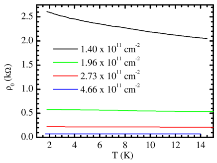
Figure 2: Temperature dependance of resistivity at four different densities

In Fig. 2 we plot the resistivity of the sample measured at $B=0$ and with varying values of $T$. Out of the four different values of the electron densities that have been considered, only the data taken at the lowest value of the density ($1.40\times 10^{11}/cm^{2}$) display a significant enhancement of the resistance as $T$ decreases. As the electron density is increased up to the value $4.66\times 10^{11}/cm^{2}$, the resistance decreases by a factor of about 40 and remains almost constant over the range of experimental $T$. As we shall discuss further below, this dependence on $T$ indicates that weak quantum interference effects are observable only in the experiment conducted at the lowest value of the density. For the other transport measurements at weak $B$, taken from the sample at the three higher densities, these effects play hardly a role of significance.

The Hall measurements at low $B$ show that the mobility of the electron gas enhances with increasing values of the carrier density in the range $(1.40-4.66)\times 10^{11}/cm^{2}$. This enhancement, which is primarily the result of screening of the potential fluctuations due to the static impurities and alloy disorder screening , indicates that for each value of the electron density we are dealing with fundamentally different impurity characteristics and, hence, with a truly different sample.

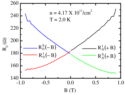
Figure 3: Asymmetric longitudinal magnetoresistance

III.2 Semiclassical regime

III.2.1 Aspects of symmetry

In Fig. 3 we plot a typical example of the effect of the polarity of the external field $B$ on the magneto resistance data, $R_{0}^{t}$ and $R_{0}^{b}$, taken from the top and the bottom pair of contacts of the Hall bar respectively. These anomalous results for opposite polarities of the $B$ field clearly display the symmetry

$$R_{0}^{t}(B)=R_{0}^{b}(-B),R_{0}^{b}(B)=R_{0}^{t}(-B)$$ (92)

that was predicted by the theory of linear density gradients, Eqs. (15) and (16). Fig. 3 therefore permits us to apply the theory of macroscopic inhomogeneities to the experimental data on the semiclassical regime. In the end we shall compare the results with those obtained from similar investigations of the quantum Hall regime.

III.2.2 Numerical estimate of density gradients

Following Eq. (20) of Section 2 we obtain the relative variation in the electron density of the sample according to

$$\frac{\delta n}{n}=2\frac{R_{H}^{r}-R_{H}^{l}}{R_{H}^{r}+R_{H}^{l}}=6.2\%.$$ (93)

It is important to emphasize that the measurements of $R_{0}^{t}-R_{0}^{b}$ and $R_{H}^{r}-R_{H}^{l}$ are fundamentally the same and therefore do not provide independent estimates for the quantity $\frac{\delta n}{n}$.

III.2.3 Nonlinear effects

We next apply Eqs (39) and (40) in order to obtain the best estimate for the local resistivity tensor. First we plot, in Fig. 4, the experimental data for $R_{0}^{t}+R_{0}^{b}$, normalized at $B=0$, with varying values of $B$ and $T$ fixed at $2K$. The data for the lowest value of the electron density, unlike those for the higher densities, show clearly a negative magneto resistance. This result is quite consistent with the statements made in the beginning which say that weak quantum interference effects are mainly displayed in the low density data and hardly significant at higher values of the electron density. Notice, however, that the data of Fig. 4, corresponding to the three higher densities, nevertheless show a weak dependence on $B$ that cannot be explained on the basis of the classical Drude-Zener-Boltzmann result for $\rho_{0}$ alone. We attribute this weak $B$-dependence in Fig. 4 to the nonlinear aspects of the density inhomogeneities that have been introduced and discussed in Section 2, notably Eq. (39). This claim can be justified, at least in a rough manner, if one compares the relative size of the linear effects, like those shown in Fig. 3, with the relative size of the nonlinear effects. On the basis of the discussion given in Section 2.3 one expects the latter to behave like the square of the former. This result qualitatively explains the $B$-dependence as observed in the transport data at the three higher densities, Fig. 4.

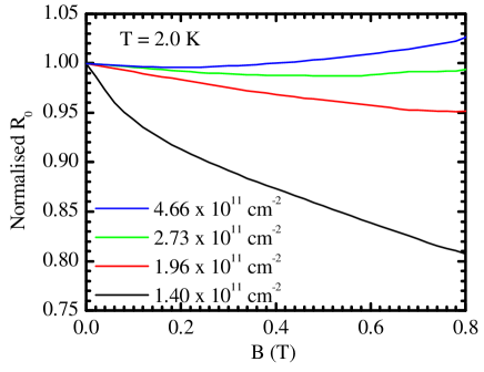
Figure 4: Normalized magneto resistance versus $B$ at $T=2K$.

In summary we can say that the effects of macroscopic inhomogeneities, inherent to the experiment, are adequately described and well accounted for by our theory of linear and nonlinear density gradients, at least as far as the semiclassical regime of transport is concerned.

III.2.4 The semicircle law

As a next step toward a better understanding of the semiclassical regime we next convert the experimental magneto resistance data into a conductivity data using the standard formulae

$$\sigma_{xx}=\frac{\rho_{0}}{\rho_{0}^{2}+\rho_{H}^{2}},~{}~{}~{}~{}~{}\sigma_{xy}=\frac{\rho_{H}}{\rho_{0}^{2}+\rho_{H}^{2}}.$$ (94)

where

$$\rho_{0}=\frac{W}{2L}(R_{0}^{t}+R_{0}^{b}),~{}~{}~{}~{}~{}\rho_{H}=\frac{1}{2}(R_{H}^{r}+R_{H}^{l}).$$ (95)

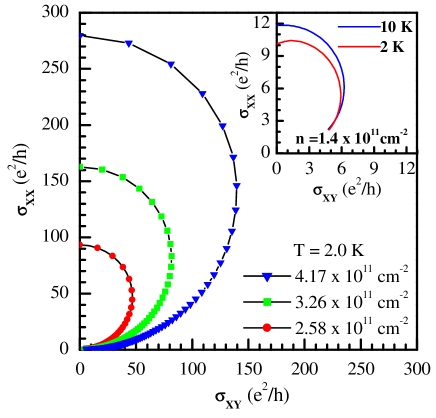
Figure 5: Experimental data (symbols) and semiclassical values (solid lines) in the $\sigma_{xx}$, $\sigma_{xy}$ conductivity plane. The inset shows the different, $T$ dependent behavior of the experimental data (solid lines) corresponding the to the lowest electron density.

In Fig. 5 we plot the results in units ($e^{2}/h$) in the $\sigma_{xx}$, $\sigma_{xy}$ conductivity plane. We observe that the data lie on nearly perfect semicircles except those corresponding to $n=1.4\times 10^{11}/cm^{2}$ which are plotted separately, in the inset of Fig. 5. The semicircles are, in fact, predicted by the well known results of Drude-Zener-Boltzmann theory

$$\sigma_{xx}=\frac{\sigma_{0}}{1+(\omega_{c}\tau)^{2}}\hskip 36.135pt\sigma_{xy}=\frac{\sigma_{0}\omega_{c}\tau}{1+(\omega_{c}\tau)^{2}}.$$ (96)

with $\sigma_{0}=1/\rho_{0}=ne^{2}{\tau}/m^{*}$. Eq. (92) implies

$$\left(\sigma_{xx}-\frac{\sigma_{0}}{2}\right)^{2}+\sigma_{xy}^{2}=\left(\frac{\sigma_{0}}{2}\right)^{2},$$ (97)

which fits the data in Fig. 5 remarkably well. Several comments are in order.

(i) Plots like Fig. 5 clearly demonstrate the fact that the semiclassical Drude-Zener-Boltzmann theory is in many ways a surprisingly successful theory over the entire range of experimental $B$. Many interesting and fundamental aspects of the electron transport problem are being suppressed, however. For example, the deviations from the semiclassical behavior, like the nonlinear effects mentioned in the discussion of Fig. 4, can no longer be observed when a data set of the same sample taken over a wide B range is plotted as in Fig. 5.

(ii) Similar statements apply to the fundamental aspects of the quantum Hall regime. These are all invisible in experimental plots of $\sigma_{xx}$ and $\sigma_{xy}$ where the scale is set by the typical values of the semiclassical theory. As is well known, the quantum Hall regime generally appears at strong values of $B$ only. This regime collapses, in Fig. 5, into an extremely small region around the origin, $\sigma_{xx}\lesssim 1$kivelson:prb92 .

(iii) All this merely illustrates the well known fact that quantum Hall regime is experimentally well separated from the semiclassical regime where the physics is mainly dominated by weak localization and interaction phenomena (Section 3.2.5 below). At strong values of $B$ the problem is in many ways very different and the role played by the macroscopic inhomogeneities will have to be considered separately (Section 3.3).

III.2.5 Semiclassical versus weak quantum interference phenomena

Next we focus on the low density data in Fig. 5 that have been plotted separately, in the inset. These data, unlike those taken at a higher values of the electron density, indicate a significant departure from the semiclassical theory of electron transport (semicircle law) as $T$ is lowered. This behavior, with varying $T$, is naturally explained within the aforementioned theory of weak localization and interaction effects. For this purpose we recall that the quantum theory can in general be written as in Eq. 80, i.e.

$$\sigma_{xx}(T)=\sigma_{xx}^{c}+\beta\ln(T/T_{f})$$ (98)

where $\beta$ and $T_{f}$ are positive constants that depend on $B$, electron spin etc. Finkel . We have introduced a superscript ’$c$’ in order to make an explicit distinction between the semiclassical theory on the one hand, and the quantum theory of conductances on the other. It is well understood by now that the theory of weak quantum interference phenomena predicts, at the same time, that the Hall component $\sigma_{xy}$ remains unchanged. We can write

$$\sigma_{xy}(T)=\sigma_{xy}=\sigma_{xy}^{c}.$$ (99)

For comparison we have plotted the data for $\sigma_{xx}$ and $\sigma_{xy}$ for two different $T$ and with varying values of $\omega_{c}\tau$ as in Fig. 6. We have made use of the relation

$$\omega_{c}\tau=B/B_{max}$$ (100)

where $B_{max}$ is defined as the value of $B$ where the data for $\sigma_{xy}$ pass through a maximum.

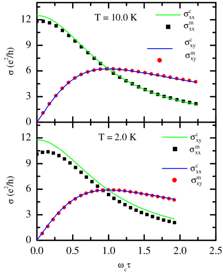
Figure 6: Experimental data (symbols) for the conductivity components $\sigma_{xx}$, $\sigma_{xy}$ for the sample with lowest density, with varying $\omega_{c}\tau$ and at two different values of $T$. The solid lines indicate the associated semiclassical values (see text).

To check the validity of Eq.99 we have fitted the data for $\sigma_{xy}$ with the semiclassical expression, Eq 96. The best fit (solid line in Fig. 6) is obtained by fixing the value of the parameter $\sigma_{0}$ at half the maximum value of $\sigma_{xy}$ and the results are listed in Table 1. Once the value of $\sigma_{0}$ is known, the semiclassical expression for $\sigma_{xx}$ is also fixed. These results have been plotted in Fig. 6 (solid line) as well. On the basis of Fig.6 we can make the following qualitative statements.

(i) Both the statements of Eqs 98 and 99 are completely consistent with the experiment. Whereas the data for $\sigma_{xy}$ follow the semiclassical predictions quite well, the data for $\sigma_{xx}$ show, as mentioned earlier, a significant departure from the semiclassical line as $T$ is lowered from $10K$ to $2K$.

(ii) Notice, however, that this departure is strongest at $\omega_{c}\tau\approx 0$ and weakest in the regime $0.5\lesssim\omega_{c}\tau\lesssim 2.0$. This is a well known result of weak quantum interference theory and indicates that at $B=0$ and $B\neq 0$ the problem generally belongs to a different universality class, i.e. the coefficient $\beta$ in Eq. 98 is different in each case.

(iii) Since the quantum corrections to $\sigma_{xx}^{c}$ are relatively small, typically O($e^{2}/h$) in the range of experimental $T$, it becomes immediately obvious why similar corrections are not observed in the other data in Fig. 5, taken from the sample at higher values of the electron densities.

(iv) Finally, it is important to emphasize that a quantitative assessment of scaling phenomena like Eq.98 is complicated, mainly because of the fact that the semiclassical parameters of the system at low densities depend on $T$ as well. In particular, the parameter $\sigma_{0}$ (Table 1) and, hence, $\sigma_{xx}^{c}$ and $\sigma_{xy}^{c}$ in Eqs 98 and 99 vary by $7\%$ in the range $2K<T<10K$. Notice that this dependence on $T$ accounts for roughly $30\%$ of the $T$ dependence as observed in the $\sigma_{xx}$ data at $\omega_{c}\tau=0$ (Fig. 6) .

A $T$ dependence of the semi classical parameters has been observed previously, on similar systems at low densitiesMinkov:prb01 . It indicates that the relaxation time $\tau$ and, hence, the ionized impurity distribution varies with varying $T$. Physically this happens because of redistribution of electrons in the doped layer which reduces the remote ion impurity scattering at higher temperatures.

In summary we can say that transport studies of the semiclassical regime provide invaluable physical information on the electron gas that cannot be obtained otherwise. It is quite obvious, for example, that the type of $T$ dependence in the sample characteristics as discussed in the present Section can have dramatic and misleading consequences for the experiments conducted at strong $B$. In particular, it can be one of the physical mechanisms that generally prevents one from observing the universal features of quantum criticality of the quantum Hall plateau transitions, notably the algebraic dependence $T^{\kappa}$.

Table 1: Numerical value of parameters entering into the semiclassical theory (see text).

Temp	$\bf B_{max}$	$\tau$	$\sigma_{0}$	n
(K)	(Tesla)	(ps)	$(\frac{e^{2}}{h})$	$(\times 10^{11}cm^{-2})$
2.0	0.52 $\pm$0.04	0.39 $\pm$0.03	11.78 $\pm$0.04	1.48 $\pm$0.12
10.0	0.45 $\pm$0.04	0.45 $\pm$0.04	12.48 $\pm$0.04	1.36 $\pm$0.12
2.0	0.11 $\pm$0.01	1.20	62.80	2.58
2.0	0.09 $\pm$0.01	2.46	162.47	3.26
2.0	0.07 $\pm$0.01	3.32	279.76	4.17

III.2.6 Numerical values of semiclassical parameters

For completeness we next present numerical estimates for the various parameters that enter into the semiclassical theory. Specifically we list, in Table 1, the values of $B_{max}$, $\tau$, $\sigma_{0}$ and $n$ for each case separately.

First, as far as the data taken at higher densities ($n=2.58,~{}3.26,~{}4.17\times~{}10^{11}cm^{-2}$) are concerned, these parameters can be extracted in a standard manner simply because the quantum corrections are negligible in this case. Specifically, we have extracted the values for $\sigma_{0}$ and $n$ directly from the experimental resistance data by using Eq.95 as well as the relations $\rho_{0}=1/\sigma_{0}$ and $\rho_{H}=B/ne$. Once the $\sigma_{0}$ and $n$ are fixed we can accurately compute the value of $\tau=\sigma_{0}m^{*}/ne^{2}$ as well. In the computation of $\tau$ the effective mass $m^{*}$ of system is considered $0.036m_{e}$. The results do not vary significantly in the range $2K<T<10K$. Along with the measured $B_{max}$ they are listed in Table 1.

Next, for the data corresponding to the lowest value of the electron density ($n=1.48,~{}1.36~{}\times~{}10^{11}cm^{-2}$) one has to follow a slightly different extraction procedure. According to the discussion following Eq.99 one can use the $\sigma_{xy}$ data and obtain an accurate value for $\sigma_{0}$ and an estimate for $B_{max}$ which is generally much less accurate, however. Given the values of $\sigma_{0}$ and $B_{max}$ one can next compute the electron density $n=\sigma_{0}B_{max}/e$ as well as the relaxation time $\tau=m^{*}/eB_{max}$. The accuracy of the computation is mainly limited by experimental uncertainties in $B_{max}$. The results obtained for $T=2K$ and $10K$ are listed in Table 1. Notice that the difference in $n$ at $2K$ and $10K$ is insignificant in view of the large error bars. On the other hand, we do attribute the $T$ dependence in $\sigma_{0}$ to the fact that $\tau$ is $T$ dependent.

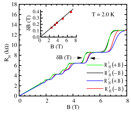
Figure 7: High field Hall resistance, inset shows the difference of critical magnetic field for PP transitions

III.3 Quantum Hall regime

III.3.1 Aspects of symmetry

We next consider the transport properties in the regime of high $B$ where the quantum features dominate for average electron density $4.17\times~{}10^{11}cm^{-2}$. Fig. 7 shows the magnitude of Hall resistances $R_{H}^{l}$ and $R_{H}^{r}$ as measured at the contacts $AB$ and $CD$ of the Hall bar with varying $B$ up to 8 Tesla and for both directions of the field. Fig. 8 shows the corresponding data of the longitudinal resistances $R_{0}^{t}$ and $R_{0}^{b}$ as measured at the contacts $AC$ and $BD$ respectively.

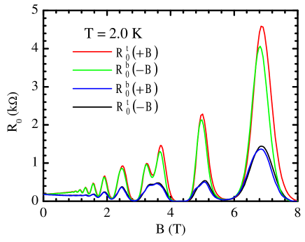
Figure 8: High field longitudinal magnetoresistance

As a first investigation of inhomogeneity effects we study the symmetry of the data under a change in the polarity of the magnetic field $B$. Following Eqs (15-17) the two sets of data for $R_{0}^{t}$ and $R_{0}^{b}$ should be related according to

$$R_{0}^{t}(+B)=R_{0}^{b}(-B),~{}~{}R_{0}^{t}(-B)=R_{0}^{b}(+B).$$ (101)

Similarly, the two sets of data for $R_{h}^{l}$ and $R_{H}^{r}$ should be related as follows

$$R_{H}^{l}(+B)=-R_{H}^{l}(-B),~{}~{}R_{H}^{r}(+B)=-R_{H}^{r}(-B).$$ (102)

From Figs 7 and 8 we observe that the statements of symmetry are all in qualitative agreement with the experiment at high $B$, indicating that the gradients in the electron density still remain the principle reason for having imperfect data.

III.3.2 Numerical estimate for density gradients

The shift in the ”critical” $B$ values for the PP transition as taken from the left contact ($AB$) and the right contact ($CD$) is directly related to the filling fraction $\nu=nh/eB$ of the Landau level system. Since the electron density $n$ varies along the channel of the Hall bar, the PP transition at the low-density side (AB) occurs at a relatively lower value for $B$ whereas at the high-density side (CD) the transition takes place at a relatively higher $B$. Notice that this is precisely the statement made by Eq. (54) which says that for fixed $T$ and varying $B$ the measured Hall resistances can be written as follows

$$R_{H}^{l}(B)=\rho_{H}(n_{l},B),~{}~{}~{}~{}R_{H}^{r}(B)=\rho_{H}(n_{r},B).$$ (103)

Here, $n_{l}$ and $n_{r}$ are the different but fixed electron densities at the left contacts ($AB$) and right contacts ($CD$) of the Hall bar respectively. Equating $R_{H}^{l}$ and $R_{H}^{r}$ amounts to taking different values $B_{l}$ and $B_{r}$ for the magnetic field $B$ at the left and the right hand side of the Hall bar such that the filling fraction is the same. Hence

$$\nu=\frac{n_{l}h}{eB_{l}}=\frac{n_{r}h}{eB_{r}}$$ (104)

from which it follows immediately that

$$\frac{\delta n}{n}=2\frac{n_{r}-n_{l}}{n_{r}+n_{l}}=2\frac{B_{r}-B_{l}}{B_{r}+B_{l}}=\frac{\delta B}{B}$$ (105)

irrespective of whether the Landau levels are spin polarized or not.

In the inset of Fig. 7 we have taken $\delta B$ as the difference in the value of $B$ where the data for $R_{H}^{l}$ and $R_{H}^{r}$ pass through the ”center” of the plateau transition. We observe that the $\delta B$ as taken from the different plateau transitions varies linearly with $B$. The slope of the line gives an estimate for the relative difference $\delta n/n$ in the electron densities at the left and right contacts of the Hall bar. More specifically we have ${\delta}B/B={\delta}n/n=6{\%}$ which agrees remarkably well with the aforementioned result ($6.2\%$) as obtained from the low $B$ data.

III.3.3 Beyond linear approximation

We have seen so far that the transport data at high $B$ do indeed display the features of symmetry as predicted by Eqs (15-17). At the same time one is also able to obtain reliable numerical estimates for the density gradients from the experimental data for both the quantum Hall regime and the semiclassical regime. This, however, does not take away from the fact that additional features are clearly present in the data that are caused by different aspects of inhomogeneity. In this Section we shall point out that a proper analysis of the experiment on the PP transitions is actually way beyond the limitations of the linear approximation. This statement becomes most obvious by looking at the quantum Hall plateau transitions in the $R_{H}^{l}$ and $R_{H}^{r}$ data (Fig. 7). Recall that the plateau transitions as observed in the $R_{H}^{l}$ and $R_{H}^{r}$ data are shifted by amount $\delta B$ in $B$ due to density gradients. This $\delta B$, however, is comparable or even larger than the actual width $\Delta B$ of the plateau transition as observed in the same data. Notice that $\Delta B\propto T^{\kappa}$ is the quantity of actual interest whereas the ratio $\frac{\delta B}{\Delta B(T)}$ is identically the same as the ratio $\frac{\delta\nu_{x}}{\nu_{0}(T)}$ introduced in Section 2.4. We therefore conclude that the present experiment is conducted in a regime of $T$ where one can no longer expect the data to provide reliable information on the quantum critical behavior of the electron gas, notably the numerical value of the critical index $\kappa$. This conclusion is entirely consistent with the experimental data on $R_{0}^{t}$ and $R_{0}^{b}$ (Fig. 8). In particular, the measured $R_{0}^{t,b}$ provide a substantially larger estimate for the width $\Delta B$ of the PP transitions than what one obtains from the $R_{H}^{l,r}$ data. This discrepancy can simply be understood from the fact that the longitudinal resistance is measured along the length of the Hall bar where the electron density changes the most. $R_{0}^{t,b}$ therefore represents an average over a range of electron densities. This is unlike the quantity $R_{H}^{l,r}$ which probes the local electron densities at the left hand side and right hand side of the Hall bar, $n_{l}$ and $n_{r}$ respectively.

These considerations simply illustrate the fact that the resistance data do not necessarily reflect the intrinsic properties of the quantum phase transition alone. Macroscopic sample inhomogeneities may enter the problem in a highly non-linear fashion and, hence, they may fundamentally complicate the studies of quantum criticality in the quantum Hall regime.

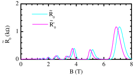
Figure 9: Plot of difference resistance $\tilde{R}_{0}$ extracted from Hall resistances at the CD contacts (Fig. 1). Also the difference resistance $\tilde{R^{\prime}}_{0}$ with B values rescaled is plotted (see text)

III.3.4 Contact misalignment

In this Section we address the small deviation from the ideal reflection symmetry, Eqs. (15-17), that can clearly be seen in the experimental data on the Hall resistance, $R_{H}$, in Fig. 7. Whereas the data for $R_{H}^{l}$ nicely display the symmetry under the change $B\rightarrow-B$, this is not so for the $R_{H}^{r}$ data which have been measured from the right hand side contacts ($CD$, Fig. 1) of the Hall bar. This asymmetry between the $R_{H}^{r}(B)$ and $R_{H}^{r}(-B)$ signals can easily be explained, however, if one assumes that the right hand side contacts $CD$, unlike the $AB$ on the left hand side, are slightly misaligned. More specifically, by assuming that the contacts $C$ and $D$ are misaligned in the x-direction by a small amount, say $\Delta<<L$, then the difference between the Hall resistances, $\tilde{R}_{0}=|R_{H}^{r}(-B)|-|R_{H}^{r}(B)|$, should be proportional to the local (near CD, Fig. 1) longitudinal resistance $R_{0}$.

To test the idea of contact misalignment we have plotted, in Fig.9, the quantity $\tilde{R}_{0}$ with varying $B$. As expected, the results look very much the same as the experimental plot of $R_{0}$, Fig. 8. One can build upon these results in several ways. For example, one thing to notice is that the peaks in the $\tilde{R}_{0}$ data corresponding to the different PP transitions are shifted towards higher $B$ values as compared to the $R_{0}$ data in Fig. 8. This shift in $B$ is a result of the fact that the $\tilde{R}_{0}$ actually probe the local longitudinal resistance of the system at CD contacts where as $R_{0}$ represents an average over a range of electron densities. For the purpose of showing this we have also plotted the results (denoted by $\tilde{R^{\prime}}_{0}$ in Fig. 9) that have been obtained from $\tilde{R}_{0}$ after a simple re-scaling of the $B$ axis with a factor $\frac{n_{r}+n_{l}}{2n_{r}}=0.967$. Here, $n_{r}$ and $n_{l}$ are the electron densities at opposite sides of the Hall bar that we have considered earlier. The peaks in $\tilde{R^{\prime}}_{0}$ and those in $R_{0}$ now occur at approximately the same values for $B$, indicating that the effect is dominated by the variations in the electron density that are linear in the spatial coordinates. For completeness we report the numerical value of the misalignment $\Delta$. On the basis of the magneto resistance measurements at low $B$ we conclude that $\Delta$ is equal to $2.5\%$ of the length of the Hall bar, $L$ (Fig. 1).

IV Summary and conclusions

We have classified and analyzed the most important effects of sample inhomogeneity on the transport data taken from low mobility heterostructures. We have shown, in particular, that the presence of density gradients manifests itself most clearly in terms of a reflection symmetry that generally exists in the longitudinal and transverse magneto resistance data taken from the symmetrically placed contacts on the Hall bar.

The expressions obtained under the so-called linear approximation allow us to extract the main features of semiclassical transport and weak quantum interference, even for samples containing a density gradient of nearly $6$ percent. Going beyond the linear approximation, we have introduced an exactly solvable model with exponential density gradients. The nonlinear inhomogeneity effects are found to be weak in the regime of semiclassical transport or weak $B$, but they generally complicate the experiments on scaling of the PP transitions. Since the sample used in the present experiments possesses density gradients which are rather large, it clearly brings out the futility of attaching meaning to the shapes and $T$ dependence of the magneto resistance measurements on the PP transitions. While it is best therefore to avoid the complications of sample inhomogeneities altogether, the analysis specifies fundamental bounds on the experimental density gradients which may be tolerated in the study of quantum criticality of both the PP and PI transitions. It is further seen that the experimental restrictions are far more severe for the PP transitions than for the PI transition taken from the same sample. These restrictions mainly place a lower limit on the experimental $T$ below which the quantum critical behavior of the electron gas can no longer be studied. Along with the density gradients, our present experiments also reveal the effects of another common aspect of inhomogeneity, the misalignment of the Hall bar contacts, that generally affects the shape and $T$ dependence of the quantum transport measurements at the PP and PI transitions.

Appendix A Aspects of symmetry

In this Appendix we point out that the universality of the scaling functions, Eqs (72-76), is actually a statement of universality made on the $\beta$ and $\gamma$ functions of the electron gas. For this purpose we recall that the Coulomb interaction problem generally involves the renormalization of three distinct parameters, namely the dimensionless conductances $\sigma_{xx}$ and $\sigma_{xy}$ as well as the singlet interaction amplitude $z$ that is associated with the variable $T$ and/or the external frequency. The most fundamental quantities of the theory are defined as follows

$$\frac{d\sigma_{xx}}{d\ln\mu} = \beta_{xx}(\sigma_{xx},\sigma_{xy})$$ (106)

$$\frac{d\sigma_{xy}}{d\ln\mu} = \beta_{xy}(\sigma_{xx},\sigma_{xy})$$ (107)

$$\frac{d\ln zT}{d\ln\mu} = 2+\gamma(\sigma_{xx},\sigma_{xy}).$$ (108)

Here, $\mu$ denotes an arbitrary momentum scale in the problem and $\gamma(\sigma_{xx},\sigma_{xy})$ is known as the anomalous dimension of the variable $z$ or $T$. The following symmetries are fundamental features of quantum Hall systems

$\bullet$  Particle-hole symmetry  

$$\beta_{xx}(\sigma_{xx},\sigma_{xy}) = ~{}\beta_{xx}(\sigma_{xx},1-\sigma_{xy})$$ (109)

$$\beta_{xy}(\sigma_{xx},\sigma_{xy}) = -\beta_{xy}(\sigma_{xx},1-\sigma_{xy})$$ (110)

$$\gamma(\sigma_{xx},\sigma_{xy}) = ~{}~{}~{}\gamma(\sigma_{xx},1-\sigma_{xy}).$$ (111)

$\bullet$  Periodicity in $\sigma_{xy}$  

$$\beta_{xx}(\sigma_{xx},\sigma_{xy}) = ~{}\beta_{xx}(\sigma_{xx},\sigma_{xy}+k)$$ (112)

$$\beta_{xy}(\sigma_{xx},\sigma_{xy}) = ~{}\beta_{xy}(\sigma_{xx},\sigma_{xy}+k)$$ (113)

$$\gamma(\sigma_{xx},\sigma_{xy}) = ~{}~{}~{}\gamma(\sigma_{xx},\sigma_{xy}+k).$$ (114)

These symmetries give rise to the general statement which says that the quantum Hall plateaus are described by a series of equivalent stable fixed points located at $\sigma_{xx}=0$ and $\sigma_{xy}=k$. At the same time, the critical singularities of the plateau transitions are controlled by a series of equivalent unstable fixed points located at precisely half-integer values of the Hall conductance.

Appendix B Experimental $\beta$ functions

To establish the contact with the experiment we introduce the following quantities

$$\frac{d\sigma_{xx}}{d\ln zT} = \frac{\beta_{xx}(\sigma_{xx},\sigma_{xy})}{2+\gamma(\sigma_{xx},\sigma_{xy})}=\tilde{\beta}_{xx}(\sigma_{xx},\sigma_{xy})$$ (115)

$$\frac{d\sigma_{xy}}{d\ln zT} = \frac{\beta_{xy}(\sigma_{xx},\sigma_{xy})}{2+\gamma(\sigma_{xx},\sigma_{xy})}=\tilde{\beta}_{xy}(\sigma_{xx},\sigma_{xy}).$$ (116)

Notice that the experimental $\tilde{\beta}_{xx}$ and $\tilde{\beta}_{xy}$ functions display the same symmetries as the original ones, $\beta_{xx}$ and $\beta_{xy}$.

Next, on the basis of Eqs (72) and (73), which are defined on the interval $0\leqq\sigma_{xy}\leqq 1$, one can obtain the explicit expressions for $\tilde{\beta}_{xx}$ and $\tilde{\beta}_{xy}$ as follows. First we solve for the quantities $X$ and $\eta$

$$X=\Phi_{odd}(\sigma_{xx},\sigma_{xy});~{}~{}~{}\eta=\Phi_{even}(\sigma_{xx},\sigma_{xy}),$$ (117)

where

$$\Phi_{even}(\sigma_{xx},\sigma_{xy}) = \frac{\frac{1}{2}-\sqrt{(\sigma_{xy}-\frac{1}{2})^{2}+\sigma_{xx}^{2}}}{\sigma_{xx}}$$ (118)

$$\Phi_{odd}(\sigma_{xx},\sigma_{xy}) = \ln\left(\frac{\sigma_{xy}-\sigma_{xx}\Phi_{even}}{\sigma_{xx}}\right).$$ (119)

Notice that

$$\Phi_{even}(\sigma_{xx},\sigma_{xy}) = ~{}~{}\Phi_{even}(\sigma_{xx},1-\sigma_{xy})$$ (120)

$$\Phi_{odd}(\sigma_{xx},\sigma_{xy}) = -\Phi_{odd}(\sigma_{xx},1-\sigma_{xy}).$$ (121)

Apparently we have

$$\frac{d\Phi_{odd}}{d\ln T} = -\kappa\Phi_{odd}$$ (122)

$$\frac{d\Phi_{even}}{d\ln T} = y_{\sigma}\Phi_{even},$$ (123)

such that $\Phi_{odd}$ and $\Phi_{even}$ can be identified as the Wegner scaling fields in the problem.

The experimental $\tilde{\beta}$ functions in the interval $0\leqq\sigma_{xy}\leqq 1$ are now obtained as follows

$$\tilde{\beta}_{xx}(\sigma_{xx},\sigma_{xy})=+2\sigma_{xx}\times$$

$$\left\{\kappa(\sigma_{xy}-\frac{1}{2})\Phi_{odd}-y_{\sigma}\sigma_{xx}\Phi_{even}\right\}$$ (124)

$$\tilde{\beta}_{xy}(\sigma_{xx},\sigma_{xy})=-2\sigma_{xx}\times$$

$$\left\{\kappa(\sigma_{xx}+\frac{1}{2}\Phi_{even})\Phi_{odd}+y_{\sigma}(\sigma_{xy}-\frac{1}{2})\Phi_{even}\right\}\qquad.$$ (125)

First, it is readily established that the result satisfies particle-hole symmetry as it should be

$$\tilde{\beta}_{xx}(\sigma_{xx},\sigma_{xy}) = ~{}\tilde{\beta}_{xx}(\sigma_{xx},1-\sigma_{xy})$$ (126)

$$\tilde{\beta}_{xy}(\sigma_{xx},\sigma_{xy}) = -\tilde{\beta}_{xy}(\sigma_{xx},1-\sigma_{xy}).$$ (127)

Secondly, we make use of the statement of periodicity in $\sigma_{xy}$, Eqs (77-79), and extend the expressions for $\tilde{\beta}$ to include the entire range of $\sigma_{xy}$, i.e.

$$\tilde{\beta}_{xx}(\sigma_{xx},\sigma_{xy}) \rightarrow ~{}\tilde{\beta}_{xx}(\sigma_{xx},\sigma_{xy}+k)$$ (128)

$$\tilde{\beta}_{xy}(\sigma_{xx},\sigma_{xy}) \rightarrow \tilde{\beta}_{xy}(\sigma_{xx},\sigma_{xy}+k).$$ (129)

As a final step we can next employ the analysis of this Section in a backwards manner and show that the solutions to the differential equations, Eqs (B.1) and (B.2), are indeed given by Eq. (77) with the parameters $T_{0}^{(k)}$ and $T_{1}^{(k)}$ being left undetermined.

References

- (1) H. P. Wei, D. C. Tsui, M. A. Palaanen, and A. M. M. Pruisken, Phys. Rev. Lett. 61, 1294 (1988).
- (2) S. W. Hwang, H. P. Wei, L. W. Engel, D. C. Tsui, and A. M. M. Pruisken, Phys. Rev. B 48, 11416 (1993).
- (3) A. M. M. Pruisken, Phys. Rev. Lett. 61, 1297 (1988).
- (4) S. Koch, R. J. Haug, K. v. Klitzing, and K. Ploog, Phys. Rev. B 43, 6828 (1991); S. Koch, R. J. Haug, K. v. Klitzing, and K. Ploog, Phys. Rev. B 46, 1596 (1992).
- (5) D. Shahar, M. Hilke, C. C. Li, D. C. Tsui, S. .L. Sondhi, J. E. Cunningham, and M. Razeghi, Solid State Comm. 107, 19 (1998); D. Shahar, D. C. Tsui, M. Shayegan, J. E. Cunningham, E. Shimshoni, and S. .L. Sondhi, Solid State Comm. 102, 817 (1997).
- (6) M. Hilke, D. Shahar, S. H. Song, D. C. Tsui, Y. H. Xie, and D. Monroe, Nature 395, 675 (1998).
- (7) T. Wang, K. P. Clark, G. F. Spencer, A. M. Mack, and W. P. Kirk, Phys. Rev. Lett. 72, 709 (1994); C. H. Lee, Y. H. Chang, Y. W. Suen, and H. H. Lin, Phys. Rev. B 56, 15238 (1997); W. Pan, D. Shahar, D. C. Tsui, H. P. Wei, and M. Razeghi, Phys. Rev. B 55, 15431 (1997); Kun Yang, D. Shahar, R. N. Bhatt, D. C. Tsui, and M. Shayegan, J. Phys.: Condens. Matter 12, 5343 (2000); S. Q. Murphy, J. L. Hicks, W. K. Liu, S. J. Chung, K. J. Goldammer, and M. B. Santos, Physica E 6, 293 (2000).
- (8) A.M.M. Pruisken, B. Škorić and M. Baranov, Phys. Rev. B60, 16838 (1999)
- (9) R. T. F. van Schaijk, A. de Visser, S. M. Olsthoorn, H. P. Wei, and A. M. M. Pruisken, Phys. Rev. Lett. 84, 1567 (2000).
- (10) A. M. M. Pruisken, D. T. N. de Lang, L. A. Ponomarenko, and A. de Visser, e-print: cond-mat/0109043, submitted to Phys. Rev. Lett.
- (11) D. T. N. de Lang, L. A. Ponomarenko, A. de Visser, C. Possanzini, S. M. Olsthoorn, and A. M. M. Pruisken, Physica E 12, 666 (2002).
- (12) A.M.M. Pruisken and M.A. Baranov, Europhys. Lett. 31 543 (1995) and references therein.
- (13) A.M. Finkelstein, Pis’ma Zh. Eksp. Teor. Fiz. 37, 436 (1983) [JETP Lett. 37, 517 (1983)]; Zh. Eksp. Teor. Fiz. 86, 367 (1984) [Sov. Phys. JETP 59, 212 (1984)]; Physica B 197, 636 (1994).
- (14) M.A. Baranov, I.S. Burmistrov, and A.M.M. Pruisken, Phys. Rev. B66, 075317 (2002)
- (15) H.P. Wei, D.C. Tsui and A.M.M. Pruisken, Phys. Rev. B33, 1488 (1985); H.P. Wei et.al., Surf. Sc. 170, 238 (1986).
- (16) See also L.A. Ponomorenko em et.al., cond-mat/0306063
- (17) R. T. Bate and A. C. Beer, J. Appl. Phys. 32, 800 (1961).
- (18) I.M. Ruzin, N.R. Cooper and B.I. Halperin, Phys. Rev. B53, 1558 (1992)
- (19) A.M.M. Pruisken et.al. unpublished.
- (20) D.G. Polyakov and B.I. Shklovskii, Phys. Rev. Lett. 73, 1150 (1994).
- (21) W. Walukiewicz et al., Phys. Rev. B 30, 4571 (1984).
- (22) S. Kivelson, D.-H. Lee, and S.-C. Zhang, Phys. Rev. B 46, 2223 (1992).
- (23) G. M. Minkov, O. E. Rut, A. V. Germanenko, and A. A. Sherstobitov, Phys. Rev. B 64, 235327 (2001).