Additivity of decoherence measures for multiqubit quantum systems

Abstract

We introduce new measures of decoherence appropriate for evaluation of quantum computing designs. Environment-induced deviation of a quantum system’s evolution from controlled dynamics is quantified by a single numerical measure. This measure is defined as a maximal norm of the density matrix deviation. We establish the property of additivity: in the regime of the onset of decoherence, the sum of the individual qubit error measures provides an estimate of the error for a several-qubit system. This property is illustrated by exact calculations for a spin-boson model.

Dynamics of open quantum systems has long been a subject of study in diverse fields open ; vanKampen . Recent interest in quantum computing has focused attention nonMarkov ; short ; Privman on quantifying environmental effects that cause small deviations from the isolated-system quantum dynamics. During short time intervals of “quantum-gate” functions, environment-induced relaxation/decoherence effects must be kept below a certain threshold in order to allow fault-tolerant quantum error correction qec . The reduced density matrix of the quantum system, with the environment traced out, is usually evaluated within some approximation scheme, e.g., apscheme . In this work, we introduce a new, additive measure of the deviation from the “ideal” density matrix of an isolated system. For a single two-state system (a qubit) this measure is calculated explicitly for the environment modeled as a bath of harmonic modes Caldeira , e.g., phonons. Furthermore, we establish that for a several-qubit system, the introduced measure of decoherence is approximately additive for short times. It can be estimated by summing up the deviation measures of the constituent qubits, without the need to carry out a many-body calculation, similar to the approximate additivity expected for relaxation rates of exponential approach to equilibrium at large times.

In most quantum computing proposals, quantum algorithms are implemented in the following way. Evolution of the qubits is governed by a Hamiltonian consisting of single-qubit operators and of two-qubit interaction terms Lloyd ; Barenco . Some parameters of the Hamiltonian can be controlled externally to implement the desired algorithm. During each cycle of the computation the Hamiltonian remains constant. This ideal model does not include the influence of the environment on the computation, which necessitates quantum error correction. The latter involves non-unitary operations qec and cannot be described as Hamiltonian-governed dynamics.

The accepted approach to evaluate environmentally induced decoherence involves a model in which each qubit is coupled to a bath of environmental modes Caldeira . The reduced density matrix of the system, with the bath modes traced out, then describes the time-dependence of the system dynamics nonMarkov ; Markov ; apscheme . Because of the interaction with environment, after each cycle the state of the qubits will be slightly different from the ideal. The resulting error accumulates at each cycle, so that large-scale quantum computation is not possible without implementing fault-tolerant error correction schemes qec ; Kitaev . These schemes require the environmentally induced decoherence of the quantum state in one cycle to be below some threshold. Its value, defined for uncorrelated single qubit error rates, was estimated PreskillDiVincenzo to be between $10^{-6}$ and $10^{-4}$.

To evaluate error rate for a given system, one should first obtain the evolution of its density operator. In realistic cases various approximations are utilized nonMarkov ; short ; Markov ; apscheme . The most familiar are the Markovian-type approximations Markov used to evaluate approach to the thermal state at large times. It has been pointed out recently that these approximations are not suitable for quantum computing purposes because they are usually not valid vanKampen ; short at low temperatures and for the short cycle times of quantum computation. Several non-Markovian approaches nonMarkov ; short ; Privman ; apscheme have been developed to evaluate the short-time dynamics of open quantum systems.

Additional issues arise when one tries to study decoherence of several-qubit systems. One has to consider the degree to which noisy environments of different qubits are correlated Storcz . If all the qubits are effectively immersed in the same bath, then there is a way to reduce decoherence for this group of qubits without error correction procedures, by encoding the state of one logical qubit in a decoherence free subspace of the states of several physical qubits Palma ; DFS . In a large scale quantum computer consisting of thousands of qubits, it is more appropriate to consider qubits immersed in distinct baths, because these errors represent the “worst case scenario” that necessitates error-correction.

Once we have the density matrix $\rho(t)$ for a single- or few-qubit system evaluated in some approximation, we have to compare it to the ideal density matrix $\rho^{(i)}(t)$ corresponding to quantum algorithm without environmental influences. We have to define some measure of decoherence, $D(t)$, to compare with the fault-tolerance criteria, which are not specific with regards to the error-rate definition qec . It is convenient to have the measure nonnegative, and vanishing if and only if the system evolves in complete isolation. Since explicit calculations beyond one or very few qubits are exceedingly difficult, it would be also useful to find a measure which is additive (or at least sub-additive), i.e., the measure of decoherence of a composite system will be the sum (or not greater than the sum) of the measures of decoherence of its subsystems. In this work, we identify two measures of decoherence which have these desirable properties. We prove the asymptotic additivity and derive explicit results for decoherence in a short-time approximation.

Typically, the Hamiltonian of an open quantum system interacting with environment has the form $H=H_{S}+H_{B}+H_{I}$, where $H_{S}$ is the internal Hamiltonian, $H_{B}$ is the Hamiltonian of the environment (bath), $H_{I}$ is the system-bath interaction term. Over gate-function cycles, and between them, the terms in $H$ will be considered constant. Therefore, the overall density matrix $R(t)$ of the system and bath evolves according to $R(t)=\exp{\left(-iHt/\hbar\right)}R(0)\exp{\left(iHt/\hbar\right)}$. Usually the initial density matrix $R(0)=\rho(0){\raise 2.0pt\hbox{$\scriptscriptstyle{\otimes}$}}\Theta$ is assumed Markov to be a direct product of the initial density matrix of the system, $\rho(0)$, and the thermalized density matrix of the bath, $\Theta$. The reduced density matrix of the system is obtained by tracing out the bath modes, $\rho(t)={\rm Tr_{B}}\,R(t)$.

To quantify the effect of the interaction with the bath norm , we consider the deviation, $\sigma(t)$, of the reduced density matrix from the ideal $\rho^{(i)}(t)\equiv\exp{\left(-iH_{S}t/\hbar\right)}\rho(0)\exp{\left(iH_{S}t/\hbar\right)}$,

$$\sigma(t)=\rho(t)-\rho^{(i)}(t).$$ (1)

As a numerical measure of the deviation we will use the operator norm $\left\|\sigma\right\|_{\lambda}$. It is defined Kato as the maximal absolute value of the eigenvalues of the matrix $\sigma$. For a $2\times 2$ deviation matrix, $\left\|\sigma\right\|_{\lambda}=(\left|{\sigma_{11}}\right|^{2}+\left|{\sigma_{12}}\right|^{2})^{1/2}$.

Note that $\left\|\sigma\right\|_{\lambda}$ is not only a function of time, but it also depends on the initial density operator $\rho(0)$. Due to decoherence, it will increase from zero as time goes by. However, its time-dependence will also contain oscillations at the frequencies of the internal system dynamics, as illustrated in Fig. 1. The effect of the bath can be better quantified by the maximal deviation norm,

$$D(t)=\sup_{\rho(0)}\big{(}\|\sigma(t,\rho(0))\|_{\lambda}\big{)}.$$ (2)

One can show that $0\leq D(t)\leq 1$. This measure of decoherence will typically increase monotonically from zero at $t=0$, saturating at large times at a value $D(\infty)\leq 1$. The definition of the maximal decoherence measure $D(t)$ looks rather complicated for a general multiqubit system. However, in what follows we show that it can be evaluated in closed form for short times, appropriate for quantum computing, for a single-qubit (two-state) system. We then establish an approximate additivity that allows us to estimate $D(t)$ for several-qubit systems as well.

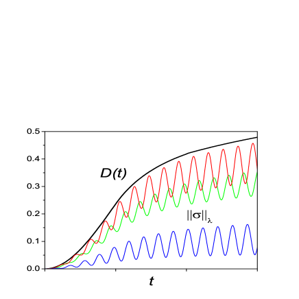
Figure 1: Schematic plot of the deviation norm for a two-level system interacting with the Ohmic bath open of bosonic modes in the short-time approximation short . The oscillatory curves illustrate the $\left\|\sigma\right\|_{\lambda}$ norms for three different initial states $\rho(0)$. The monotonic curve shows the $D$ norm, obtained as $\left\|\sigma\right\|_{\lambda}$ maximized (2) over $\rho(0)$. Note that in this case $D(\infty)=1/2$.

To be specific, let us outline the calculation of this measure of decoherence of a two-level system (spin, qubit) interacting with a bosonic bath of modes. Thus, we take

$$H_{S} = {-(\hbar\Omega/2)}\sigma_{z},\quad H_{B}=\hbox{$\sum_{k}$}{\hbar\omega_{k}a_{k}^{\dagger}a_{k}^{\vphantom{\dagger}}},$$ (3)

$$H_{I} = \sigma_{x}\hbox{$\sum_{k}$}{(g_{k}^{\vphantom{\dagger}}a_{k}^{\dagger}+g_{k}^{*\vphantom{\dagger}}a_{k}^{\vphantom{\dagger}})}.$$ (4)

Here $\omega_{k}$ are the bath mode frequencies, $a_{k}^{\vphantom{\dagger}},\,a_{k}^{\dagger}$ are the bosonic annihilation and creation operators, $g_{k}$ are the coupling constants, $\sigma_{x}$ and $\sigma_{z}$ are the Pauli matrices, and $\hbar\Omega>0$ is the energy gap between the ground (up, $|1\rangle$) and excited (down, $|2\rangle$) states of the qubit.

The dynamics of the system can be obtained in closed form in the short-time approximation short . The expression for the density operator of a spin-1/2 system is

$$\rho_{mn}(t)\! = \!\!\hbox{$\sum\limits_{{p,q=1,2\atop\mu,\nu=\pm 1}}$}{}\rho_{pq}(0)\langle m|\mu\rangle\langle\mu|p\rangle\langle q|\nu\rangle\langle\nu|n\rangle$$ (5)

$$\times e^{i[(E_{q}+E_{n}-E_{p}-E_{m})t/2-B^{2}(t)(\eta_{\mu}-\eta_{\nu})^{2}/4]}.$$

Here the Roman-labeled states, $|j\rangle$, with $j=m,n,p,q=1,2$, are the eigenstates of $H_{S}$ corresponding to the eigenvalues $E_{j}/\hbar=(-1)^{j}\Omega/2$. The Greek-labeled states, $|\zeta\rangle$, are the eigenstates of $\sigma_{x}$, with the eigenvalues $\eta_{\zeta}=\zeta$, where $\zeta=\mu,\nu=\pm 1$. The spectral function $B^{2}(t)$ is defined according to

$$B^{2}(t)=8\hbox{$\sum_{k}$}{}{{\left|{g_{k}}\right|^{2}}}{{\omega_{k}^{-2}}}\sin^{2}({{{\omega_{k}t}/{2}}})\coth({{{\beta\omega_{k}}/2)}}.$$ (6)

Here $\beta=\hbar/k_{B}T$, $k_{B}$ is the Boltzmann constant, and $T$ is the initial bath temperature. This function has been studied in Palma ; vanKampen ; basis . With $\rho_{12}(0)=|\rho_{12}(0)|e^{i\phi}$, we get

$$\left\|\sigma(t)\right\|_{\lambda} = \hbox{$\frac{1}{2}$}\big{[}1-e^{-B^{2}(t)}\big{]}\big{\{}[\rho_{11}(0)-\rho_{22}(0)]^{2}$$ (7)

$$+ 4\left|\rho_{12}(0)\right|^{2}\sin^{2}[(\Omega/2)t+\phi]\big{\}}^{1/2}.$$

In Fig. 1, we show schematically the behavior of $\left\|\sigma(t)\right\|_{\lambda}$ for three representative choices of the initial density matrix $\rho(0)$. Generally, $\left\|\sigma(t)\right\|_{\lambda}$ increases with time, reflecting the decoherence of the system. However, oscillations at the system’s internal frequency $\Omega$ are superimposed, as seen explicitly in (7).

The effect of the bath is better quantified by the maximal operator norm $D(t)$. In order to maximize over $\rho(0)$, we can parameterize $\rho(0)=U\left(P|1\rangle\langle 1|+(1-P)|2\rangle\langle 2|\right)U^{\dagger}$, where $0\leq P\leq 1$, and $U$ is an arbitrary $2\times 2$ unitary matrix,

$$U=\left(\begin{array}[]{cc}e^{i(\alpha+\gamma)}\cos\theta&e^{i(\alpha-\gamma)}\sin\theta\\ -e^{i(\gamma-\alpha)}\sin\theta&e^{-i(\alpha+\gamma)}\cos\theta\\ \end{array}\right).$$ (8)

By using the rigorous definition Kato of the norm, $\left\|A\right\|_{\lambda}^{2}=\mathop{\sup}_{\psi\neq 0}(\langle\psi|A^{\dagger}A|\psi\rangle/\langle\psi|\psi\rangle)$, one can show that it suffices to put $P=1$ and search for the maximum over the remaining three real parameters $\alpha$, $\gamma$ and $\theta$. The result, sketched in Fig. 1, is

$$D(t)=\hbox{$\frac{1}{2}$}\big{[}1-e^{-B^{2}(t)}\big{]}.$$ (9)

In quantum computing, the error rates can be significantly reduced by using several physical qubits to encode each logical qubit DFS . Therefore, even before active quantum error correction is incorporated qec , evaluation of decoherence of several qubits is an important, but formidable task. Consider a system consisting of two initially unentangled subsystems $S_{1}$ and $S_{2}$, with decoherence norms $D_{S_{1}}$ and $D_{S_{2}}$, respectively. We denote the density matrix of the full system as $\rho_{S_{1}S_{2}}$ and its deviation as $\sigma_{S_{1}S_{2}}$, and use a similar notation with subscripts $S_{1}$ and $S_{2}$ for the two subsystems. If the evolution of system is governed by the “noninteracting” Hamiltonian of the form $H_{S_{1}S_{2}}=H_{S_{1}}+H_{S_{2}}$, where the terms $H_{S_{1}}$, $H_{S_{2}}$ act only on variables of the system $S_{1}$, $S_{2}$, respectively, then the overall norm $D_{S_{1}S_{2}}$ can be bounded by the sum of the norms $D_{S_{1}}$ and $D_{S_{2}}$,

$$D_{S_{1}S_{2}}^{\vphantom{(i)}}=\sup_{\rho(0)}\|\sigma_{S_{1}S_{2}}^{\vphantom{(i)}}\|_{\lambda}=\sup_{\rho(0)}\|\rho_{S_{1}S_{2}}^{\vphantom{(i)}}-\rho^{(i)}_{S_{1}S_{2}}\|_{\lambda}=$$ (10)

$$\sup_{\rho(0)}\|\rho_{S_{1}}^{\vphantom{(i)}}\!{\raise 2.0pt\hbox{$\scriptscriptstyle{\otimes}$}}\rho_{S_{2}}^{\vphantom{(i)}}\!-\rho_{S_{1}}^{(i)}{\raise 2.0pt\hbox{$\scriptscriptstyle{\otimes}$}}\rho_{S_{2}}^{(i)}\|_{\lambda}=\sup_{\rho(0)}\|\sigma_{S_{1}}^{\vphantom{(i)}}\!{\raise 2.0pt\hbox{$\scriptscriptstyle{\otimes}$}}\rho_{S_{2}}^{\vphantom{(i)}}\!+\rho_{S_{1}}^{(i)}{\raise 2.0pt\hbox{$\scriptscriptstyle{\otimes}$}}\sigma_{S_{2}}^{\vphantom{(i)}}\|_{\lambda}$$

$$\leq\sup_{\rho(0)}\|\sigma_{S_{1}}^{\vphantom{(i)}}{\raise 2.0pt\hbox{$\scriptscriptstyle{\otimes}$}}\rho_{S_{2}}^{\vphantom{(i)}}\|_{\lambda}+\sup_{\rho(0)}\|\rho_{S_{1}}^{(i)}{\raise 2.0pt\hbox{$\scriptscriptstyle{\otimes}$}}\sigma_{S_{2}}^{\vphantom{(i)}}\|_{\lambda}$$

$$\leq\sup_{\rho_{S_{1}}(0)}\|\sigma_{S_{1}}^{\vphantom{(i)}}\|_{\lambda}+\sup_{\rho_{S_{2}}(0)}\|\sigma_{S_{2}}^{\vphantom{(i)}}\|_{\lambda}=D_{S_{1}}^{\vphantom{(i)}}+D_{S_{2}}^{\vphantom{(i)}}.$$

In general, initially unentangled qubits will remain nearly unentangled for short times, because they didn’t have enough time to interact. Therefore, the inequality $D_{S_{1}S_{2}}\lesssim D_{S_{1}}+D_{S_{2}}$ is expected to provide a good approximate estimate for $D_{S_{1}S_{2}}$, i.e., the measures for individual qubits can be considered approximately additive. For large times, the separate measures become of order 1, so this bound is not useful. Instead, the rates of approach of various quantities to their asymptotic values are approximately additive in some cases. In the rest of this work, we focus on the short-time regime, of no significant interaction effects, and establish a much stronger property: We prove the approximate additivity for initially entangled qubits whose dynamics is governed by (3-4) with coupling to independent baths.

For intermediate calculations, we use the “diamond” norm introduced by Kitaev Kitaev , which we denote by $K$,

$$K(t)=\|T-T^{(i)}\|_{\diamond}=\underset{{\varrho}}{\sup}\|\{[T-T^{(i)}]{\raise 2.0pt\hbox{$\scriptscriptstyle{\otimes}$}}I_{G}\}{\varrho}\|_{\rm Tr}.$$ (11)

Here, the trace norm Kato is given by $\left\|A\right\|_{\rm Tr}={\rm Tr}\,\sqrt{A^{\dagger}A}$. The two superoperators are defined as generating the actual and “ideal” dynamical evolutions,

$$T(t):\rho(0)\mapsto\rho(t),\quad T^{(i)}(t):\rho(0)\mapsto\rho^{(i)}(t),$$ (12)

$I_{G}$ is the identity superoperator on a Hilbert space $G$ whose dimension is the same as that of the corresponding space of the superoperators $T$ and $T^{(i)}$, and $\varrho$ is a density operator in this space of twice the number of qubits.

Consider again the composite system consisting of the two subsystems $S_{1}$, $S_{2}$, with the “noninteracting” Hamiltonian $H_{S_{1}S_{2}}=H_{S_{1}}+H_{S_{2}}$. The evolution superoperator of the system will be $T_{S_{1}S_{2}}=T_{S_{1}}{\raise 2.0pt\hbox{$\scriptscriptstyle{\otimes}$}}T_{S_{2}}$, and the ideal one will be $T_{S_{1}S_{2}}^{(i)}=T_{S_{1}}^{(i)}{\raise 2.0pt\hbox{$\scriptscriptstyle{\otimes}$}}T_{S_{2}}^{(i)}$. The diamond measure for the whole system can be expressed Kitaev as

$$K_{S_{1}S_{2}}^{\vphantom{(i)}}=\|T_{S_{1}S_{2}}^{\vphantom{(i)}}-T_{S_{1}S_{2}}^{(i)}\|_{\diamond}=$$

$$\|(T_{S_{1}}^{\vphantom{(i)}}-T_{S_{1}}^{(i)}){\raise 2.0pt\hbox{$\scriptscriptstyle{\otimes}$}}T_{S_{2}}^{\vphantom{(i)}}+T_{S_{1}}^{(i)}{\raise 2.0pt\hbox{$\scriptscriptstyle{\otimes}$}}(T_{S_{2}}^{\vphantom{(i)}}-T_{S_{2}}^{(i)})\|_{\diamond}$$

$$\leq\|(T_{S_{1}}^{\vphantom{(i)}}-T_{S_{1}}^{(i)}){\raise 2.0pt\hbox{$\scriptscriptstyle{\otimes}$}}T_{S_{2}}^{\vphantom{(i)}}\|_{\diamond}+\|T_{S_{1}}^{(i)}{\raise 2.0pt\hbox{$\scriptscriptstyle{\otimes}$}}(T_{S_{2}}^{\vphantom{(i)}}-T_{S_{2}}^{(i)})\|_{\diamond}=$$

$$\|T_{S_{1}}^{\vphantom{(i)}}-T_{S_{1}}^{(i)}\|_{\diamond}\|T_{S_{2}}^{\vphantom{(i)}}\|_{\diamond}+\|T_{S_{1}}^{(i)}\|_{\diamond}\|T_{S_{2}}^{\vphantom{(i)}}-T_{S_{2}}^{(i)}\|_{\diamond}=$$

$$\|T_{S_{1}}^{\vphantom{(i)}}-T_{S_{1}}^{(i)}\|_{\diamond}+\|T_{S_{2}}^{\vphantom{(i)}}-T_{S_{2}}^{(i)}\|_{\diamond}=K_{S_{1}}^{\vphantom{(i)}}+K_{S_{2}}^{\vphantom{(i)}}.$$ (13)

The step that follows the inequality, in (13), proved in Kitaev as the “stability” property, was established specifically with the definition (11).

The approximate inequality $K_{S_{1}S_{2}}\lesssim K_{S_{1}}+K_{S_{2}}$ for the diamond norm $K$ has thus the same form as for the norm $D$. Let us emphasize that both relations apply assuming that for short times the subsystem interactions, directly with each other or via their coupling to the bath modes, have had no significant effect. However, there is an important difference that the relation for $D$ further requires the subsystems to be initially unentangled. This restriction does not apply to the relation for $K$. This property is particularly useful for quantum computing, which is based on qubit entanglement. However, even in the simplest case of the diamond norm of one qubit, the calculations are extremely cumbersome. Therefore, the measure $D$ is favorable for actual calculations.

In general, one can prove that $2D(t)\leq K(t)\leq 2$. For a single qubit, calculation within the short-time approximation actually gives $K(t)=2D(t)$. Since $D$ is generally bounded by $K/2$, it follows that for the specific model considered, with a bosonic heat bath acting independently on each of the qubits, the multiqubit norm $D$ is approximately bounded from above by the sum of the single-qubit norms even for the initially entangled qubits:

$$D\leq K/2\lesssim\hbox{$\sum_{j}$}K_{j}/2=\hbox{$\sum_{j}$}(1-e^{-B^{2}_{j}})/2=\hbox{$\sum_{j}D_{j}$},$$ (14)

where $j=1,\ldots,N$ labels the qubits.

For short times, one can also establish a lower bound on $D(t)$. Consider a specific initial state with all the qubits excited, $\rho(0)=(|2\rangle\langle 2|)_{1}{\raise 2.0pt\hbox{$\scriptscriptstyle{\otimes}$}}\ldots{\raise 2.0pt\hbox{$\scriptscriptstyle{\otimes}$}}(|2\rangle\langle 2|)_{N}$. Then according to (5), $\rho(t)=\rho_{1}(t){{\raise 2.0pt\hbox{$\scriptscriptstyle{\otimes}$}}}\ldots{\raise 2.0pt\hbox{$\scriptscriptstyle{\otimes}$}}\rho_{N}(t)$, where $\rho_{j}(t)=(1/2)\big{\{}\big{[}1-e^{-B^{2}_{j}(t)}\big{]}|1\rangle\langle 1|+\big{[}1+e^{-B^{2}_{j}(t)}\big{]}|2\rangle\langle 2|\big{\}}$. The right-bottom matrix element of the (diagonal) deviation operator, $\sigma_{2^{N},2^{N}}(t)=-1+2^{-N}{\prod_{j}}[1+e^{-B^{2}_{j}(t)}]$, can be expanded as $({1}/{2})\sum_{j}B_{j}^{2}(t)+o(\sum_{j}B_{j}^{2}(t))$, because $B(t)$ is linear in $t$ for small times. The largest eigenvalue of $\sigma(t)$ cannot be smaller than $\sigma_{2^{N},2^{N}}(t)$. It follows that

$$D\geq\hbox{$\frac{1}{2}$}\hbox{$\sum_{j}$}B^{2}_{j}+o\big{(}\hbox{$\sum_{j}$}B_{j}^{2}\big{)}=\hbox{$\sum_{j}$}D_{j}+o\big{(}\hbox{$\sum_{j}$}D_{j}\big{)},$$ (15)

where we used (9) for short times.

By combining the upper and lower bounds, we get the final result for short times,

$$D(t)=\hbox{$\sum_{j}$}D_{j}(t)+o\big{(}\hbox{$\sum_{j}$}D_{j}(t)\big{)}.$$ (16)

This completes the proof of additivity of the measure $D(t)$ at short times, for spin-qubits interacting with bosonic environmental modes. This result should apply as a good approximation up to intermediate, inverse-system-energy-gap times, e.g., short , and it is consistent with the recent finding Dalton that at short times decoherence of a trapped-ion quantum computer scales approximately linearly with the number of qubits.

- (1) G.W. Ford, M. Kac and P. Mazur, J. Math. Phys. 6, 504 (1965); A.O. Caldeira and A.J. Leggett, Physica A 121, 587 (1983); S. Chakravarty and A.J. Leggett, Phys. Rev. Lett. 52, 5 (1984); A.J. Leggett, S. Chakravarty, A.T. Dorsey, M.P.A. Fisher and W. Zwerger, Rev. Mod. Phys. 59, 1 (1987); H. Grabert, P. Schramm and G.-L. Ingold, Phys. Rep. 168, 115 (1988).
- (2) N.G. van Kampen, J. Stat. Phys. 78, 299 (1995).
- (3) K.M. Fonseca Romero and M.C. Nemes, Phys. Lett. A 235, 432 (1997); C. Anastopoulos and B.L. Hu, Phys. Rev. A 62, 033821 (2000); G.W. Ford and R.F. O’Connell, Phys. Rev. D 64, 105020 (2001); D. Braun, F. Haake, and W.T. Strunz, Phys. Rev. Lett. 86, 2913 (2001); G.W. Ford, J.T. Lewis, and R.F. O’Connell, Phys. Rev. A 64, 032101 (2001); J. Wang, H.E. Ruda and B. Qiao, Phys. Lett. A 294, 6 (2002); E. Lutz, cond-mat/0208503; A. Khaetskii, D. Loss and L. Glazman, Phys. Rev. B 67, 195329 (2003); R.F. O’Connell and J. Zuo, Phys. Rev. A 67, 062107 (2003), W.T. Strunz, F. Haake and D. Braun, Phys. Rev. A 67, 022101 (2003); W.T. Strunz and F. Haake, Phys. Rev. A 67, 022102 (2003); V. Privman, D. Mozyrsky and I.D. Vagner, Comp. Phys. Commun. 146, 331 (2002).
- (4) V. Privman, J. Stat. Phys. 110, 957 (2003).
- (5) V. Privman, Mod. Phys. Lett. B 16, 459 (2002).
- (6) P.W. Shor, Phys. Rev. A 52, R2493 (1995); A.M. Steane, Phys. Rev. Lett. 77, 793 (1996); C.H. Bennett, G. Brassard, S. Popescu, B. Schumacher, J.A. Smolin and W.K. Wootters, Phys. Rev. Lett. 76, 722 (1996); A.R. Calderbank and P.W. Shor, Phys. Rev. A 54, 1098 (1996); A.M. Steane, Phys. Rev. A 54, 4741 (1996); D. Aharonov and M. Ben-Or, quant-ph/9611025; D. Gottesman, Phys. Rev. A 54, 1862 (1997); E. Knill and R. Laflamme, Phys. Rev. A 55, 900 (1997).
- (7) D. Loss and D.P. DiVincenzo, cond-mat/0304118; V. Privman, Proc. SPIE 5115, 345 (2003); W.H. Zurek, Rev. Mod. Phys. 75, 715 (2003).
- (8) A.O. Caldeira and A.J. Leggett, Phys. Rev. Lett. 46, 211 (1981).
- (9) S. Lloyd, Phys. Rev. Lett. 75, 346 (1995).
- (10) A. Barenco, C.H. Bennett, R. Cleve, D.P. DiVincenzo, N. Margolus, P. Shor, T. Sleator, J.A. Smolin and H. Weinfurter, Phys. Rev. A 52, 3457 (1995).
- (11) N.G. van Kampen, Stochastic Processes in Physics and Chemistry, North-Holland, 2001; W.H. Louisell, Quantum Statistical Properties of Radiation, Wiley, 1973; K. Blum, Density Matrix Theory and Applications, Plenum, 1996; A. Abragam, The Principles of Nuclear Magnetism, Clarendon Press, 1983.
- (12) A.Y. Kitaev, Russ. Math. Surv. 52, 1191 (1997); D. Aharonov, A. Kitaev and N. Nisan, Proc. XXXth ACM Symp. Theor. Comp., Dallas, TX, USA, 20 (1998); A.Yu. Kitaev, A.H. Shen and M.N. Vyalyi, Classical and Quantum Computation, AMS, 2002.
- (13) J. Preskill, Proc. Roy. Soc. Lond. A 454, 385 (1998); D.P. DiVincenzo, Fort. Phys. 48, 771 (2000).
- (14) M.J. Storcz and F.K. Wilhelm, Phys. Rev. A 67, 042319 (2003).
- (15) G.M. Palma, K.A. Suominen and A.K. Ekert, Proc. Roy. Soc. Lond. A 452, 567 (1996).
- (16) L.-M. Duan and G.-C. Guo, Phys. Rev. Lett. 79, 1953 (1997); P. Zanardi and M. Rasetti, Phys. Rev. Lett. 79, 3306 (1997); D.A. Lidar, I.L. Chuang and K.B. Whaley, Phys. Rev. Lett. 81, 2594 (1998).
- (17) L. Fedichkin, A. Fedorov and V. Privman, Proc. SPIE 5105, 243 (2003).
- (18) T. Kato, Perturbation Theory for Linear Operators, Springer-Verlag, NY, 1995.
- (19) D. Mozyrsky and V. Privman, J. Stat. Phys. 91, 787 (1998).
- (20) B.J. Dalton, J. Mod. Opt. 50, 951 (2003).